Reproducing Key Figures from Kay et al. (2015)

Overview¶

This notebook demonstrates how one might use the NCAR Community Earth System Model (CESM) Large Ensemble (LENS) data hosted on AWS S3. The notebook shows how to reproduce figures 2 and 4 from the Kay et al. (2015) paper describing the CESM LENS dataset Kay et al., 2015.

This resource is intended to be helpful for people not familiar with elements of the Pangeo framework including Jupyter Notebooks, Xarray, and Zarr data format, or with the original paper, so it includes additional explanation.

Prerequisites¶

Concepts	Importance	Notes
Intro to Xarray	Necessary
Dask	Helpful

Time to learn: 30 minutes

NOTE: In this notebook, we access very large cloud-served datasets and use Dask to parallelize our workflow. The end-to-end execution time may be on the order of an hour or more, depending on your computing resources.

Imports¶

import sys
import warnings
warnings.filterwarnings("ignore")

import intake
import matplotlib.pyplot as plt
from dask.distributed import Client
import numpy as np
import pandas as pd
import xarray as xr
import cmaps  # for NCL colormaps
import cartopy.crs as ccrs
import dask
import s3fs

dask.config.set({"distributed.scheduler.worker-saturation": 1.0})

<dask.config.set at 0x7ff9ecf01e90>

Create and Connect to Dask Distributed Cluster¶

Here we’ll use a dask cluster to parallelize our analysis.

platform = sys.platform

if (platform == 'win32'):
    import multiprocessing.popen_spawn_win32
else:
    import multiprocessing.popen_spawn_posix

client = Client()
client

Load and Prepare Data¶

catalog_url = 'https://ncar-cesm-lens.s3-us-west-2.amazonaws.com/catalogs/aws-cesm1-le.json'
col = intake.open_esm_datastore(catalog_url)
col

Show the first few lines of the catalog:

col.df.head(10)

Show expanded version of collection structure with details:

col.keys_info().head()

Extract data needed to construct Figure 2¶

Search the catalog to find the desired data, in this case the reference height temperature of the atmosphere, at daily time resolution, for the Historical, 20th Century, and RCP8.5 (IPCC Representative Concentration Pathway 8.5) experiments.

col_subset = col.search(frequency=["daily", "monthly"], component="atm", variable="TREFHT",
                        experiment=["20C", "RCP85", "HIST"])

col_subset

col_subset.df

Load catalog entries for subset into a dictionary of Xarray Datasets:

dsets = col_subset.to_dataset_dict(zarr_kwargs={"consolidated": True}, storage_options={"anon": True})
print(f"\nDataset dictionary keys:\n {dsets.keys()}")

Define Xarray Datasets corresponding to the three experiments:

ds_HIST = dsets['atm.HIST.monthly']
ds_20C = dsets['atm.20C.daily']
ds_RCP85 = dsets['atm.RCP85.daily']

Use the dask.distributed utility function to display size of each dataset:

from dask.utils import format_bytes
print(f"Historical: {format_bytes(ds_HIST.nbytes)}\n"
      f"20th Century: {format_bytes(ds_20C.nbytes)}\n"
      f"RCP8.5: {format_bytes(ds_RCP85.nbytes)}")

Historical: 177.21 MiB
20th Century: 258.65 GiB
RCP8.5: 285.71 GiB

Now, extract the Reference Height Temperature data variable:

t_hist = ds_HIST["TREFHT"]
t_20c = ds_20C["TREFHT"]
t_rcp = ds_RCP85["TREFHT"]
t_20c

The global surface temperature anomaly was computed relative to the 1961-90 base period in the Kay et al. paper, so extract that time slice:

t_ref = t_20c.sel(time=slice("1961", "1990"))

Figure 2¶

Read grid cell areas¶

Cell size varies with latitude, so this must be accounted for when computing the global mean.

cat = col.search(frequency="static", component="atm", experiment=["20C"])
_, grid = cat.to_dataset_dict(aggregate=False, storage_options={'anon':True}, zarr_kwargs={"consolidated": True}).popitem()
grid

cell_area = grid.area.load()
total_area = cell_area.sum()
cell_area

Define weighted means¶

Note: resample(time="AS") does an annual resampling based on start of calendar year. See documentation for Pandas resampling options.

t_ref_ts = (
    (t_ref.resample(time="AS").mean("time") * cell_area).sum(dim=("lat", "lon"))
    / total_area
).mean(dim=("time", "member_id"))

t_hist_ts = (
    (t_hist.resample(time="AS").mean("time") * cell_area).sum(dim=("lat", "lon"))
) / total_area

t_20c_ts = (
    (t_20c.resample(time="AS").mean("time") * cell_area).sum(dim=("lat", "lon"))
) / total_area

t_rcp_ts = (
    (t_rcp.resample(time="AS").mean("time") * cell_area).sum(dim=("lat", "lon"))
) / total_area

Read data and compute means¶

Dask’s “lazy execution” philosophy means that until this point we have not actually read the bulk of the data. Steps 1, 3, and 4 take a while to complete, so we include the Notebook “cell magic” directive %%time to display elapsed and CPU times after computation.

Step 1 (takes a while)

%%time
# this cell takes a while, be patient
t_ref_mean = t_ref_ts.load()
t_ref_mean

Step 2 (executes quickly)

%%time 
t_hist_ts_df = t_hist_ts.to_series().T
#t_hist_ts_df.head()

CPU times: user 321 ms, sys: 36.2 ms, total: 357 ms
Wall time: 1.35 s

Step 3 (takes even longer than Step 1)

%%time
t_20c_ts_df = t_20c_ts.to_series().unstack().T
t_20c_ts_df.head()

Step 4 (similar to Step 3 in its execution time)

%%time
# This also takes a while
t_rcp_ts_df = t_rcp_ts.to_series().unstack().T
t_rcp_ts_df.head()

Get observations for Figure 2 (HadCRUT4)¶

The HadCRUT4 temperature dataset is described by Morice et al. (2012).

Observational time series data for comparison with ensemble average:

obsDataURL = "https://www.esrl.noaa.gov/psd/thredds/dodsC/Datasets/cru/hadcrut4/air.mon.anom.median.nc"
ds = xr.open_dataset(obsDataURL).load()
ds

def weighted_temporal_mean(ds):
    """
    weight by days in each month
    """
    time_bound_diff = ds.time_bnds.diff(dim="nbnds")[:, 0]
    wgts = time_bound_diff.groupby("time.year") / time_bound_diff.groupby(
        "time.year"
    ).sum(xr.ALL_DIMS)
    obs = ds["air"]
    cond = obs.isnull()
    ones = xr.where(cond, 0.0, 1.0)
    obs_sum = (obs * wgts).resample(time="AS").sum(dim="time")
    ones_out = (ones * wgts).resample(time="AS").sum(dim="time")
    obs_s = (obs_sum / ones_out).mean(("lat", "lon")).to_series()
    return obs_s

Limit observations to 20th century:

obs_s = weighted_temporal_mean(ds)
obs_s = obs_s['1920':]
obs_s.head()

time
1920-01-01   -0.262006
1921-01-01   -0.195891
1922-01-01   -0.301986
1923-01-01   -0.269062
1924-01-01   -0.292857
Freq: YS-JAN, dtype: float64

all_ts_anom = pd.concat([t_20c_ts_df, t_rcp_ts_df]) - t_ref_mean.data
years = [val.year for val in all_ts_anom.index]
obs_years = [val.year for val in obs_s.index]

Combine ensemble member 1 data from historical and 20th century experiments:

hist_anom = t_hist_ts_df - t_ref_mean.data
member1 = pd.concat([hist_anom.iloc[:-2], all_ts_anom.iloc[:,0]], verify_integrity=True)
member1_years = [val.year for val in member1.index]

Plotting Figure 2¶

Global surface temperature anomaly (1961-90 base period) for individual ensemble members, and observations:

ax = plt.axes()

ax.tick_params(right=True, top=True, direction="out", length=6, width=2, grid_alpha=0.5)
ax.plot(years, all_ts_anom.iloc[:,1:], color="grey")
ax.plot(obs_years, obs_s['1920':], color="red")
ax.plot(member1_years, member1, color="black")


ax.text(
    0.35,
    0.4,
    "observations",
    verticalalignment="bottom",
    horizontalalignment="left",
    transform=ax.transAxes,
    color="red",
    fontsize=10,
)
ax.text(
    0.35,
    0.33,
    "members 2-40",
    verticalalignment="bottom",
    horizontalalignment="left",
    transform=ax.transAxes,
    color="grey",
    fontsize=10,
)
ax.text(
    0.05,
    0.2,
    "member 1",
    verticalalignment="bottom",
    horizontalalignment="left",
    transform=ax.transAxes,
    color="black",
    fontsize=10,
)

ax.set_xticks([1850, 1920, 1950, 2000, 2050, 2100])
plt.ylim(-1, 5)
plt.xlim(1850, 2100)
plt.ylabel("Global Surface\nTemperature Anomaly (K)")
plt.show()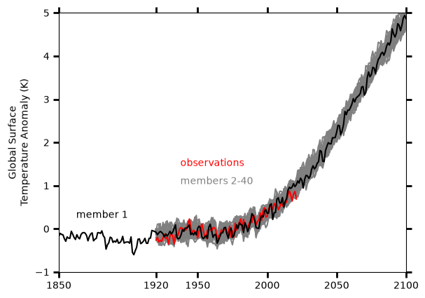

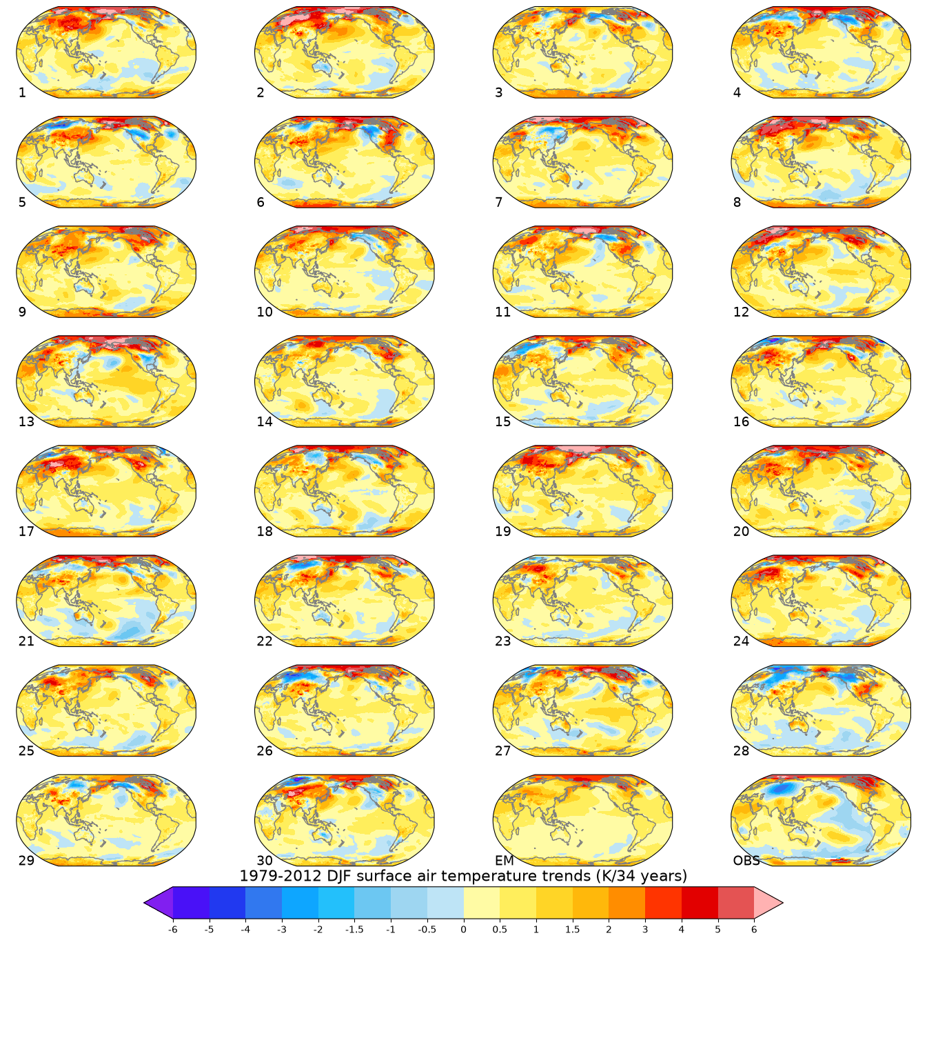
Figure 4¶

Compute linear trend for winter seasons¶

def linear_trend(da, dim="time"):
    da_chunk = da.chunk({dim: -1})
    trend = xr.apply_ufunc(
        calc_slope,
        da_chunk,
        vectorize=True,
        input_core_dims=[[dim]],
        output_core_dims=[[]],
        output_dtypes=[np.float64],
        dask="parallelized",
    )
    return trend


def calc_slope(y):
    """ufunc to be used by linear_trend"""
    x = np.arange(len(y))

    # drop missing values (NaNs) from x and y
    finite_indexes = ~np.isnan(y)
    slope = np.nan if (np.sum(finite_indexes) < 2) else np.polyfit(x[finite_indexes], y[finite_indexes], 1)[0]
    return slope

Compute ensemble trends¶

%%time 
# Takes several minutes
t = xr.concat([t_20c, t_rcp], dim="time")
seasons = t.sel(time=slice("1979", "2012")).resample(time="QS-DEC").mean("time")
# Include only full seasons from 1979 and 2012
seasons = seasons.sel(time=slice("1979", "2012")).load()

CPU times: user 29.1 s, sys: 6.5 s, total: 35.6 s
Wall time: 5min 50s

winter_seasons = seasons.sel(
    time=seasons.time.where(seasons.time.dt.month == 12, drop=True)
)
winter_trends = linear_trend(
    winter_seasons.chunk({"lat": 20, "lon": 20, "time": -1})
).load() * len(winter_seasons.time)

# Compute ensemble mean from the first 30 members
winter_trends_mean = winter_trends.isel(member_id=range(30)).mean(dim='member_id')

Make sure that we have 34 seasons:

assert len(winter_seasons.time) == 34

Get observations for Figure 4 (NASA GISS GisTemp)¶

This is observational time series data for comparison with ensemble average. Here we are using the GISS Surface Temperature Analysis (GISTEMP v4) from NASA’s Goddard Institute of Space Studies Lenssen et al., 2019.

Define the URL to Project Pythia’s Jetstream2 Object Store and the path to the Zarr file.

URL = 'https://js2.jetstream-cloud.org:8001'
filePath = 's3://pythia/gistemp1200_GHCNv4_ERSSTv5.zarr'

Create a container for the S3 file system

fs = s3fs.S3FileSystem(anon=True, client_kwargs=dict(endpoint_url=URL))

Link to the Zarr file as it exists on the S3 object store

store = s3fs.S3Map(root=filePath, s3=fs, check=False )

ds = xr.open_zarr(store, consolidated=True, chunks="auto")
ds

Create an Xarray Dataset from the Zarr object

Remap longitude range from [-180, 180] to [0, 360] for plotting purposes:

ds = ds.assign_coords(lon=((ds.lon + 360) % 360)).sortby('lon')
ds

Compute observed trends¶

Include only full seasons from 1979 through 2012:

obs_seasons = ds.sel(time=slice("1979", "2012")).resample(time="QS-DEC").mean("time")
obs_seasons = obs_seasons.sel(time=slice("1979", "2012")).load()
obs_winter_seasons = obs_seasons.sel(
    time=obs_seasons.time.where(obs_seasons.time.dt.month == 12, drop=True)
)
obs_winter_seasons

And compute observed winter trends:

obs_winter_trends = linear_trend(
    obs_winter_seasons.chunk({"lat": 20, "lon": 20, "time": -1})
).load() * len(obs_winter_seasons.time)
obs_winter_trends

Plotting Figure 4¶

Global maps of historical (1979 - 2012) boreal winter (DJF) surface air trends:

contour_levels = [-6, -5, -4, -3, -2, -1.5, -1, -0.5, 0, 0.5, 1, 1.5, 2, 3, 4, 5, 6]
color_map = cmaps.ncl_default

def make_map_plot(nplot_rows, nplot_cols, plot_index, data, plot_label):
    """ Create a single map subplot. """
    ax = plt.subplot(nplot_rows, nplot_cols, plot_index, projection = ccrs.Robinson(central_longitude = 180))
    cplot = plt.contourf(lons, lats, data,
                         levels = contour_levels,
                         cmap = color_map,
                         extend = 'both',
                         transform = ccrs.PlateCarree())
    ax.coastlines(color = 'grey')
    ax.text(0.01, 0.01, plot_label, fontsize = 14, transform = ax.transAxes)
    return cplot, ax

%%time
# Generate plot (may take a while as many individual maps are generated)
numPlotRows = 8
numPlotCols = 4
figWidth = 20
figHeight = 30

fig, axs = plt.subplots(numPlotRows, numPlotCols, figsize=(figWidth,figHeight))

lats = winter_trends.lat
lons = winter_trends.lon

# Create ensemble member plots
for ensemble_index in range(30):
    plot_data = winter_trends.isel(member_id = ensemble_index)
    plot_index = ensemble_index + 1
    plot_label = str(plot_index)
    plotRow = ensemble_index // numPlotCols
    plotCol = ensemble_index % numPlotCols
    # Retain axes objects for figure colorbar
    cplot, axs[plotRow, plotCol] = make_map_plot(numPlotRows, numPlotCols, plot_index, plot_data, plot_label)

# Create plots for the ensemble mean, observations, and a figure color bar.
cplot, axs[7,2] = make_map_plot(numPlotRows, numPlotCols, 31, winter_trends_mean, 'EM')

lats = obs_winter_trends.lat
lons = obs_winter_trends.lon
cplot, axs[7,3] = make_map_plot(numPlotRows, numPlotCols, 32, obs_winter_trends.tempanomaly, 'OBS')

cbar = fig.colorbar(cplot, ax=axs, orientation='horizontal', shrink = 0.7, pad = 0.02)
cbar.ax.set_title('1979-2012 DJF surface air temperature trends (K/34 years)', fontsize = 16)
cbar.set_ticks(contour_levels)
cbar.set_ticklabels(contour_levels)

CPU times: user 1min 17s, sys: 2.57 s, total: 1min 20s
Wall time: 1min 17s

Close our client:

client.close()

Summary¶

In this notebook, we used CESM LENS data hosted on AWS to recreate two key figures in the paper that describes the project.

What’s next?¶

More example workflows using these datasets may be added in the future.

References¶

Kay, J. E., Deser, C., Phillips, A., Mai, A., Hannay, C., Strand, G., Arblaster, J. M., Bates, S. C., Danabasoglu, G., Edwards, J., Holland, M., Kushner, P., Lamarque, J.-F., Lawrence, D., Lindsday, K., Middleton, A., Munoz, E., Neale, R., Oleson, K., … Vertenstein, M. (2015). The Community Earth System Model (CESM) Large Ensemble Project. Bull. Amer. Meteor. Soc. 10.1175/BAMS-D-13-00255.1
Morice, C. P., Kennedy, J. J., Rayner, N. A., & Jones, P. D. (2012). Quantifying uncertainties in global and regional temperature change using an ensemble of observational estimates: The HadCRUT4 data set. J. Geophys. Res. Atmos., 117(D8). 10.1029/2011JD017187
Lenssen, N., Schmidt, G., Hansen, J., Menne, M., Persin, A., Ruedy, R., & Zyss, D. (2019). Improvements in the GISTEMP uncertainty model. Journal of Geophysical Research: Atmospheres, 124(12), 6307–6326. 10.1029/2018JD029522

Foundations

Enhanced Intake-ESM Catalog Demo