Kerchunk and Pangeo-Forge

Overview

In this tutorial we are going to use Kerchunk to create reference files of a dataset. This allows us to read an entire dataset as if it were a single Zarr store instead of a collection of NetCDF files. Using Kerchunk, we don’t have to create a copy of the data, instead we create a collection of reference files, so that the original data files can be read as if they were Zarr.

This notebook shares some similarities with the Multi-File Datasets with Kerchunk, as they both create references from NetCDF files. However, this notebook differs as it uses Pangeo-Forge as the runner to create the reference files.

Prerequisites

Concepts	Importance	Notes
Kerchunk Basics	Required	Core
Multiple Files and Kerchunk	Required	Core
Kerchunk and Dask	Required	Core
Multi-File Datasets with Kerchunk	Required	IO/Visualization

Time to learn: 45 minutes

Motivation

Why Kerchunk

For many traditional data processing pipelines, the start involves download a large amount of files to a local computer and then subsetting them for future analysis. Kerchunk gives us two large advantages:

A massive reduction in used disk space.
Performance improvements with through parallel, chunk-specific access of the dataset.

In addition to these speedups, once the consolidated Kerchunk reference file has been created, it can be easily shared for other users to access the dataset.

Pangeo-Forge & Kerchunk

Pangeo-Forge is a community project to build reproducible cloud-native ARCO (Analysis-Ready-Cloud-Optimized) datasets. The Python library (pangeo-forge-recipes) is the ETL pipeline to process these datasets or “recipes”. While a majority of the recipes convert a legacy format such as NetCDF to Zarr stores, pangeo-forge-recipes can also use Kerchunk under the hood to create reference recipes.

It is important to note that Kerchunk can be used independently of pangeo-forge-recipes and in this example, pangeo-forge-recipes is acting as the runner for Kerchunk.

Why Pangeo-Forge & Kerchunk

While you can use Kerchunk without pangeo-forge, we hope that pangeo-forge can be another tool to create sharable ARCO datasets using Kerchunk. A few potential benefits of creating Kerchunk based reference recipes with pangeo-forge may include:

Recipe processing pipelines may be more standardized than case-by-case custom Kerchunk processing functions.
Recipe processing can be scaled through pangeo-forge-cloud for large datasets.
The infrastructure of pangeo-forge in GitHub may allow more community feedback on recipes.
Additional features such as appending to datasets as new data is generated may be available in future releases of pangeo-forge.

Getting to Know The Data

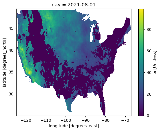
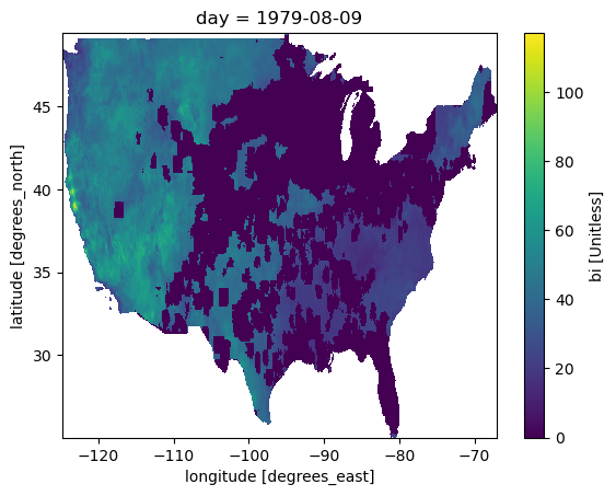
gridMET is a high-resolution daily meteorological dataset covering CONUS from 1979-2023. It is produced by the Climatology Lab at UC Merced. In this example, we are going to look create a virtual Zarr dataset of a derived variable, Burn Index.

Examine a Single File

import xarray as xr

ds = xr.open_dataset(
    "http://thredds.northwestknowledge.net:8080/thredds/dodsC/MET/bi/bi_2021.nc"
)

Plot the Dataset

ds.sel(day="2021-08-01").burning_index_g.plot()

<matplotlib.collections.QuadMesh at 0x7fe665827d30>

../../_images/836cd871569da49aa0a6c4589e22a0e8e1ad5520001a1e22743c023acd2222c1.png

Create a File Pattern

To build our pangeo-forge pipeline, we need to create a FilePattern object, which is composed of all of our input urls. This dataset ranges from 1979 through 2023 and is composed of one year per file.

To speed up our example, we will prune our recipe to select the first two entries in the FilePattern

from pangeo_forge_recipes.patterns import ConcatDim, FilePattern, MergeDim

years = list(range(1979, 2022 + 1))

time_dim = ConcatDim("time", keys=years)

def format_function(time):
    return f"http://www.northwestknowledge.net/metdata/data/bi_{time}.nc"

pattern = FilePattern(format_function, time_dim, file_type="netcdf4")

pattern = pattern.prune()

pattern

<FilePattern {'time': 2}>

Create a Location For Output

We write to local storage for this example, but the reference file could also be shared via cloud storage.

target_root = "references"
store_name = "Pangeo_Forge"

Build the Pangeo-Forge Beam Pipeline

Next, we will chain together a bunch of methods to create a Pangeo-Forge - Apache Beam pipeline. Processing steps are chained together with the pipe operator (|). Once the pipeline is built, it can be ran in the following cell.

The steps are as follows:

Creates a starting collection of our input file patterns.
Passes those file_patterns to OpenWithKerchunk, which creates references of each file.
Combines the references files into a single reference file with CombineReferences.
Writes the combined reference file.

Note: You can add additional processing steps in this pipeline.

import apache_beam as beam
from pangeo_forge_recipes.transforms import (
    OpenWithKerchunk,
    WriteCombinedReference,
)

transforms = (
    # Create a beam PCollection from our input file pattern
    beam.Create(pattern.items())
    # Open with Kerchunk and create references for each file
    | OpenWithKerchunk(file_type=pattern.file_type)
    # Use Kerchunk's `MultiZarrToZarr` functionality to combine and then write references.
    # *Note*: Setting the correct contact_dims and identical_dims is important.
    | WriteCombinedReference(
        target_root=target_root,
        store_name=store_name,
        concat_dims=["day"],
        identical_dims=["lat", "lon", "crs"],
    )
)

%%time

with beam.Pipeline() as p:
    p | transforms

CPU times: user 1.64 s, sys: 209 ms, total: 1.85 s
Wall time: 20.4 s

import os

import fsspec

full_path = os.path.join(target_root, store_name, "reference.json")
print(os.path.getsize(full_path) / 1e6)

0.048115

Our reference .json file is about 1MB, instead of 108GBs. That is quite the storage savings!

Access Speed Benchmark - Kerchunk vs NetCDF

In the access test below, we had almost a 3x speedup in access time using the Kerchunk reference dataset vs the NetCDF file collection. This isn’t a huge speed-up, but will vary a lot depending on chunking schema, access patterns etc.

Kerchunk	Time (s)
Kerchunk	10
Cloud NetCDF	28

NetCDF Cloud Access

# prepare urls
def url_gen(year):
    return (
        f"http://thredds.northwestknowledge.net:8080/thredds/dodsC/MET/bi/bi_{year}.nc"
    )


urls_list = [url_gen(year) for year in years]

%%time
netcdf_ds = xr.open_mfdataset(urls_list, engine="netcdf4")
netcdf_ds.sel(lat=slice(48, 47), lon=slice(-123, -122)).burning_index_g.mean().values

CPU times: user 1.17 s, sys: 206 ms, total: 1.37 s
Wall time: 23.5 s

array(11.726682, dtype=float32)

That took about about 28 seconds.

netcdf_ds

<xarray.Dataset>
Dimensions:          (lat: 585, lon: 1386, crs: 1, day: 16071)
Coordinates:
  * lat              (lat) float64 49.4 49.36 49.32 49.28 ... 25.15 25.11 25.07
  * lon              (lon) float64 -124.8 -124.7 -124.7 ... -67.14 -67.1 -67.06
  * crs              (crs) float32 3.0
  * day              (day) datetime64[ns] 1979-01-01 1979-01-02 ... 2022-12-31
Data variables:
    burning_index_g  (day, lat, lon) float32 dask.array<chunksize=(365, 585, 1386), meta=np.ndarray>
Attributes: (12/19)
    geospatial_bounds_crs:      EPSG:4326
    Conventions:                CF-1.6
    geospatial_bounds:          POLYGON((-124.7666666333333 49.40000000000000...
    geospatial_lat_min:         25.066666666666666
    geospatial_lat_max:         49.40000000000000
    geospatial_lon_min:         -124.7666666333333
    ...                         ...
    date:                       02 July 2019
    note1:                      The projection information for this file is: ...
    note2:                      Citation: Abatzoglou, J.T., 2013, Development...
    note3:                      Data in slices after last_permanent_slice (1-...
    note4:                      Data in slices after last_provisional_slice (...
    note5:                      Days correspond approximately to calendar day...

Storage Benchmark - Kerchunk vs NetCDF

5200x Storage Savings

Storage	Mb (s)
Kerchunk	10
Cloud NetCDF	52122

# Kerchunk Reference File
import os

print(f"{round(os.path.getsize(kerchunk_path) / 1e6, 1)} Mb")

0.0 Mb

# NetCDF Files
print(f"{round(netcdf_ds.nbytes/1e6,1)} Mb")
print("or")
print(f"{round(netcdf_ds.nbytes/1e9,1)} Gb")

52122.3 Mb
or
52.1 Gb