Multi-File Datasets with Kerchunk

Overview

This notebook is intends to build off of the Kerchunk Basics notebook.

In this tutorial we will:

Create a list of input paths for a collection of NetCDF files stored on the cloud.
Iterate through our file input list and create Kerchunk reference .jsons for each file.
Combine the reference .jsons into a single combined dataset reference with the rechunker class, MultiZarrToZarr
Learn how to read the combined dataset using Xarray and fsspec.

Prerequisites

Concepts	Importance	Notes
Kerchunk Basics	Required	Basic features
Introduction to Xarray	Recommended	IO

Time to learn: 60 minutes

Flags

In the section below, set the subset flag to be True (default) or False depending if you want this notebook to process the full file list. If set to True, then a subset of the file list will be processed (Recommended)

subset_flag = True

Imports

In our imports block we are using similar imports to the Kerchunk Basics Tutorial, with a few libraries added.

fsspec for reading and writing to remote file systems
ujson for writing Kerchunk reference files as .json
Xarray for visualizing and examining our datasets
Kerchunk's SingleHdf5ToZarr and MultiZarrToZarr classes.
tqdm for timing cell progress

from tempfile import TemporaryDirectory

import fsspec
import ujson
import xarray as xr
from kerchunk.combine import MultiZarrToZarr
from kerchunk.hdf import SingleHdf5ToZarr
from tqdm import tqdm

Create a File Pattern from a list of input NetCDF files

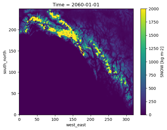
Below we will create a list of input files we want Kerchunk to index. In the Kerchunk Basics Tutorial, we looked at a single file of climate downscaled data over Southern Alaska. In this example, we will build off of that work and use Kerchunk to combine multiple NetCDF files of this dataset into a virtual dataset that can be read as if it were a Zarr store - without copying any data.

Specifically, in the cell below, we use fsspec to create a s3 filesystem to read the NetCDF files and a local file system to write our reference files to. You can, alternatively, write to a cloud filesystem instead of a local one, or even just keep the reference sets in temporary memory without writing at all.

After that, we use the fsspec fs_read s3 filesystem’s glob method to create a list of files matching a file pattern. We supply the base url of s3://wrf-se-ak-ar5/ccsm/rcp85/daily/2060/, which is pointing to an AWS public bucket, for daily rcp85 ccsm downscaled data for the year 2060. After this base url, we tacked on *, which acts as a wildcard for all the files in the directory. We should expect 365 daily NetCDF files.

Finally, we are appending the string s3:// to the list of return files. This will ensure the list of files we get back are s3 urls and can be read by Kerchunk.

# Initiate fsspec filesystems for reading and writing
fs_read = fsspec.filesystem("s3", anon=True, skip_instance_cache=True)
fs_write = fsspec.filesystem("")

# Retrieve list of available days in archive for the year 2060.
files_paths = fs_read.glob("s3://wrf-se-ak-ar5/ccsm/rcp85/daily/2060/*")

# Here we prepend the prefix 's3://', which points to AWS.
file_pattern = sorted(["s3://" + f for f in files_paths])

As a quick check, it looks like we have a list 365 file paths, which should be a year of downscaled climte data.

print(f"{len(file_pattern)} file paths were retrieved.")

365 file paths were retrieved.

# If the subset_flag == True (default), the list of input files will be subset to speed up the processing
if subset_flag:
    file_pattern = file_pattern[0:4]

Optional: If you want to examine one NetCDF files before creating the `Kerchunk` index, try uncommenting this code snippet below.

## Note: Optional piece of code to view one of the NetCDF files using Xarray as fsspec.

# import s3fs

# fs = fsspec.filesystem("s3",anon=True)
# ds = xr.open_dataset(fs.open(file_pattern[0]))

Create `Kerchunk` References for every file in the `File_Pattern` list

Now that we have a list of NetCDF files, we can use Kerchunk to create reference files for each one of these. To do this, we will iterate through each file and create a reference .json. To speed this process up, you could use Dask to parallelize this.

Define kwargs for `fsspec`

In the cell below, we are creating a dictionary of kwargs to pass to fsspec and the s3 filesystem. Details on this can be found in the Kerchunk Basics Tutorial in the (Define kwargs for fsspec) section. In addition, we are creating a temporary directory to store our reference files in.

so = dict(mode="rb", anon=True, default_fill_cache=False, default_cache_type="first")
output_dir = "./"

# We are creating a temporary directory to store the .json reference files
# Alternately, you could write these to cloud storage.
td = TemporaryDirectory()
temp_dir = td.name
temp_dir

'/tmp/tmppbhwcggo'

In the cell below, we are reusing some of the functionality from the previous tutorial. First we are defining a function named: generate_json_reference. This function:

Uses an fsspec s3 filesystem to read in a NetCDF from a given url.
Generates a Kerchunk index using the SingleHdf5ToZarr Kerchunk method.
Creates a simplified filename using some string slicing.
Uses the local filesytem created with fsspec to write the Kerchunk index to a .json reference file.

Below the generate_json_reference function we created, we have a simple for loop that iterates through our list of NetCDF file urls and passes them to our generate_json_reference function, which appends the name of each .json reference file to a list named output_files.

# Use Kerchunk's `SingleHdf5ToZarr` method to create a `Kerchunk` index from a NetCDF file.
def generate_json_reference(u, temp_dir: str):
    with fs_read.open(u, **so) as infile:
        h5chunks = SingleHdf5ToZarr(infile, u, inline_threshold=300)
        fname = u.split("/")[-1].strip(".nc")
        outf = f"{fname}.json"
        with open(outf, "wb") as f:
            f.write(ujson.dumps(h5chunks.translate()).encode())
        return outf


# Iterate through filelist to generate Kerchunked files. Good use for `Dask`
output_files = []
for fil in tqdm(file_pattern):
    outf = generate_json_reference(fil, temp_dir)
    output_files.append(outf)

  0%|          | 0/4 [00:00<?, ?it/s]

 25%|██▌       | 1/4 [00:18<00:56, 18.97s/it]

 50%|█████     | 2/4 [00:38<00:38, 19.25s/it]

 75%|███████▌  | 3/4 [00:57<00:19, 19.38s/it]

100%|██████████| 4/4 [01:17<00:00, 19.40s/it]

100%|██████████| 4/4 [01:17<00:00, 19.35s/it]

Here we can view the generated list of output `Kerchunk` reference files

output_files

['WRFDS_2060-01-01.json',
 'WRFDS_2060-01-02.json',
 'WRFDS_2060-01-03.json',
 'WRFDS_2060-01-04.json']

Combine `.json` `Kerchunk` reference files and write a combined `Kerchunk` reference dataset.

After we have generated a Kerchunk reference file for each NetCDF file, we can combine these into a single virtual dataset using Kerchunk's MultiZarrToZarr method.

Note that it is not strictly necessary write the reference sets of the individual input files to JSON, or to save these for later. However, in typical workflows, it may be useful to access individual datasets, or to repeat the combine step below in new ways, so we recommend writing and keeping these files.

In our example below we are passing in our list of reference files (output_files), along with concat_dims and identical_dims.

concat_dims should be a list of the name(s) of the dimensions(s) that you want to concatenate along. In our example, our input files were single time steps. Because of this, we will concatenate along the Time axis only.
identical_dims are variables that are shared across all the input files. They should not vary across the files.

After using MultiZarrToZarr to combine the reference files, we will call .translate() to store this combined reference dataset into memory. Note: by passing filename to .translate(), you can write the combined Kerchunk multi-file dataset to disk as a .json file, but we choose to do this as an explicit separate step.

ex: mzz.translate(filename='combined_reference.json')

# combine individual references into single consolidated reference
mzz = MultiZarrToZarr(
    output_files,
    concat_dims=["Time"],
    identical_dims=["XLONG", "XLAT", "interp_levels"],
)


multi_kerchunk = mzz.translate()

/usr/share/miniconda3/envs/kerchunk-cookbook-dev/lib/python3.10/site-packages/kerchunk/combine.py:269: UserWarning: Concatenated coordinate 'Time' contains less than expectednumber of values across the datasets: [0]
  warnings.warn(

Write combined kerchunk index for future use

If we want to keep the combined reference information in memory as well as write the file to .json, we can run the code snippet below.

# Write kerchunk .json record
output_fname = "combined_kerchunk.json"
with open(f"{output_fname}", "wb") as f:
    f.write(ujson.dumps(multi_kerchunk).encode())

Plot a slice of the dataset

Here we are using Xarray to select a single time slice of the dataset and plot a map of snow cover over South East Alaska.

ds.isel(Time=0).SNOW.plot()

<matplotlib.collections.QuadMesh at 0x7f769ab28370>

../../_images/70dff75159037f3bf290cda235596114a884b0c5ebd3f5f0a2fa67eb2158ca31.png

Multi-File Datasets with Kerchunk

Overview

Prerequisites

Flags

Imports

Create a File Pattern from a list of input NetCDF files

As a quick check, it looks like we have a list 365 file paths, which should be a year of downscaled climte data.

Optional: If you want to examine one NetCDF files before creating the `Kerchunk` index, try uncommenting this code snippet below.

Create `Kerchunk` References for every file in the `File_Pattern` list

Define kwargs for `fsspec`

Here we can view the generated list of output `Kerchunk` reference files

Combine `.json` `Kerchunk` reference files and write a combined `Kerchunk` reference dataset.

Write combined kerchunk index for future use

Using the output

Open combined `Kerchunk` dataset with `fsspec` and `Xarray`

Plot a slice of the dataset

Multi-File Datasets with Kerchunk

Overview

Prerequisites

Flags

Imports

Create a File Pattern from a list of input NetCDF files

As a quick check, it looks like we have a list 365 file paths, which should be a year of downscaled climte data.

Optional: If you want to examine one NetCDF files before creating the Kerchunk index, try uncommenting this code snippet below.

Create Kerchunk References for every file in the File_Pattern list

Define kwargs for fsspec

Here we can view the generated list of output Kerchunk reference files

Combine .json Kerchunk reference files and write a combined Kerchunk reference dataset.

Write combined kerchunk index for future use

Using the output

Open combined Kerchunk dataset with fsspec and Xarray

Plot a slice of the dataset

Optional: If you want to examine one NetCDF files before creating the `Kerchunk` index, try uncommenting this code snippet below.

Create `Kerchunk` References for every file in the `File_Pattern` list

Define kwargs for `fsspec`

Here we can view the generated list of output `Kerchunk` reference files

Combine `.json` `Kerchunk` reference files and write a combined `Kerchunk` reference dataset.

Open combined `Kerchunk` dataset with `fsspec` and `Xarray`