
Data Ingestion - Microsoft Planetary Computer
Overview
In this notebook, you will ingest Landsat data for use in machine learning. Machine learning tasks often involve a lot of data, and in Python, data is typically stored in memory as simple NumPy arrays. However, higher-level containers built on top of NumPy arrays provide more functionality for multidimensional gridded data (xarray) or out-of-core and distributed data (Dask). Our goal for data ingestion will be to load specific Landsat data of interest into one of these higher-level containers.
Microsoft Plantery Computer is one of several providers of Landsat Data. We are using it together with pystac-client and odc-stac because together they provide a nice Python API for searching and loading with specific criteria such as spatial area, datetime, Landsat mission, and cloud coverage.
Earth science datasets are often stored on remote servers that may be too large to download locally. Therefore, in this cookbook, we will focus primarily on ingestion approaches that load small portions of data from a remote source, as needed. However, the approach for your own work will depend not only on data size and location but also the intended analysis, so in a follow up notebook, you will see alternative approaches to loading data.
Prerequisites
Concepts |
Importance |
Notes |
|---|---|---|
Necessary |
Background |
|
Helpful |
Background |
|
Helpful |
Consult as needed |
|
Helpful |
Consult as needed |
|
Necessary |
||
Helpful |
||
Helpful |
Time to learn: 10 minutes
Imports
# Data
import odc.stac
import pandas as pd
import planetary_computer
import pystac_client
import xarray as xr
from pystac.extensions.eo import EOExtension as eo
# Viz
import hvplot.xarray
import panel as pn
pn.extension()
Open and read the root of the STAC catalog
catalog = pystac_client.Client.open(
"https://planetarycomputer.microsoft.com/api/stac/v1",
modifier=planetary_computer.sign_inplace,
)
catalog.title
'Microsoft Planetary Computer STAC API'
Microsoft Planetary Computer has a public STAC metadata but the actual data assets are in private Azure Blob Storage containers and require authentication. pystac-client provides a modifier keyword that we can use to manually sign the item. Otherwise, we’d get an error when trying to access the asset.
Search for Landsat Data
Let’s say that an analysis we want to run requires landsat data over a specific region and from a specific time period. We can use our catalog to search for assets that fit our search criteria.
First, let’s find the name of the landsat dataset. This page is a nice resource for browsing the available collections, but we can also just search the catalog for ‘landsat’:
all_collections = [i.id for i in catalog.get_collections()]
landsat_collections = [
collection for collection in all_collections if "landsat" in collection
]
landsat_collections
---------------------------------------------------------------------------
HTTPError Traceback (most recent call last)
Cell In[3], line 1
----> 1 all_collections = [i.id for i in catalog.get_collections()]
2 landsat_collections = [
3 collection for collection in all_collections if "landsat" in collection
4 ]
5 landsat_collections
Cell In[3], line 1, in <listcomp>(.0)
----> 1 all_collections = [i.id for i in catalog.get_collections()]
2 landsat_collections = [
3 collection for collection in all_collections if "landsat" in collection
4 ]
5 landsat_collections
File ~/miniconda3/envs/cookbook-dev/lib/python3.10/site-packages/pystac_client/client.py:433, in Client.get_collections(self)
429 for col in page["collections"]:
430 collection = CollectionClient.from_dict(
431 col, root=self, modifier=self.modifier
432 )
--> 433 call_modifier(self.modifier, collection)
434 yield collection
435 else:
File ~/miniconda3/envs/cookbook-dev/lib/python3.10/site-packages/pystac_client/_utils.py:18, in call_modifier(modifier, obj)
15 if modifier is None:
16 return None
---> 18 result = modifier(obj)
19 if result is not None and result is not obj:
20 warnings.warn(
21 f"modifier '{modifier}' returned a result that's being ignored. "
22 "You should ensure that 'modifier' is operating in-place and use "
23 "a function that returns 'None' or silence this warning.",
24 IgnoredResultWarning,
25 )
File ~/miniconda3/envs/cookbook-dev/lib/python3.10/site-packages/planetary_computer/sas.py:109, in sign_inplace(obj)
103 def sign_inplace(obj: Any) -> Any:
104 """
105 Sign the object in place.
106
107 See :func:`planetary_computer.sign` for more.
108 """
--> 109 return sign(obj, copy=False)
File ~/miniconda3/envs/cookbook-dev/lib/python3.10/functools.py:889, in singledispatch.<locals>.wrapper(*args, **kw)
885 if not args:
886 raise TypeError(f'{funcname} requires at least '
887 '1 positional argument')
--> 889 return dispatch(args[0].__class__)(*args, **kw)
File ~/miniconda3/envs/cookbook-dev/lib/python3.10/site-packages/planetary_computer/sas.py:367, in sign_collection(collection, copy)
364 collection.assets = deepcopy(assets)
366 for key in collection.assets:
--> 367 _sign_asset_in_place(collection.assets[key])
368 return collection
File ~/miniconda3/envs/cookbook-dev/lib/python3.10/site-packages/planetary_computer/sas.py:261, in _sign_asset_in_place(asset)
251 """Sign a PySTAC asset
252
253 Args:
(...)
258 with a signed version.
259 """
260 asset.href = sign(asset.href)
--> 261 _sign_fsspec_asset_in_place(asset)
262 return asset
File ~/miniconda3/envs/cookbook-dev/lib/python3.10/site-packages/planetary_computer/sas.py:298, in _sign_fsspec_asset_in_place(asset)
296 container = parse_adlfs_url(href)
297 if account and container:
--> 298 token = get_token(account, container)
299 storage_options["credential"] = token.token
File ~/miniconda3/envs/cookbook-dev/lib/python3.10/site-packages/planetary_computer/sas.py:470, in get_token(account_name, container_name, retry_total, retry_backoff_factor)
461 session.mount("https://", adapter)
462 response = session.get(
463 token_request_url,
464 headers=(
(...)
468 ),
469 )
--> 470 response.raise_for_status()
472 token = SASToken(**response.json())
473 if not token:
File ~/miniconda3/envs/cookbook-dev/lib/python3.10/site-packages/requests/models.py:1021, in Response.raise_for_status(self)
1016 http_error_msg = (
1017 f"{self.status_code} Server Error: {reason} for url: {self.url}"
1018 )
1020 if http_error_msg:
-> 1021 raise HTTPError(http_error_msg, response=self)
HTTPError: 404 Client Error: Not Found for url: https://planetarycomputer.microsoft.com/api/sas/v1/token/pcstacitems/items
We’ll use the landsat-c2-l2 dataset, which stands for Collection 2 Level-2. It contains data from several landsat missions and has better data quality than Level 1 (landsat-c2-l1). Microsoft Planetary Computer has descriptions of Level 1 and Level 2, but a direct and succinct comparison can be found in this community post, and the information can be verified with USGS.
Now, let’s set our search parameters. You may already know the bounding box (region/area of interest) coordinates, but if you don’t, there are many useful tools like bboxfinder.com that can help.
bbox = [-118.89, 38.54, -118.57, 38.84] # Region over a lake in Nevada, USA
datetime = "2017-06-01/2017-09-30" # Summer months of 2017
collection = "landsat-c2-l2"
We can also specify other parameters in the query, such as a specific landsat mission and the max percent of cloud cover:
platform = "landsat-8"
cloudy_less_than = 1 # percent
Now we run the search and list the results:
search = catalog.search(
collections=["landsat-c2-l2"],
bbox=bbox,
datetime=datetime,
query={"eo:cloud_cover": {"lt": cloudy_less_than}, "platform": {"in": [platform]}},
)
items = search.get_all_items()
print(f"Returned {len(items)} Items:")
item_id = {(i, item.id): i for i, item in enumerate(items)}
item_id
/home/runner/miniconda3/envs/cookbook-dev/lib/python3.10/site-packages/pystac_client/item_search.py:849: FutureWarning: get_all_items() is deprecated, use item_collection() instead.
warnings.warn(
Returned 3 Items:
{(0, 'LC08_L2SP_042033_20170718_02_T1'): 0,
(1, 'LC08_L2SP_042033_20170702_02_T1'): 1,
(2, 'LC08_L2SP_042033_20170616_02_T1'): 2}
It looks like there were three image stacks taken by Landsat 8 over this spatial region during the summer months of 2017 that has less than 1 percent cloud cover.
Preview Results and Select a Dataset
Before loading one of the available image stacks, it would be useful to get a visual check of the results. Many datasets have a rendered preview or thumbnail image that can be accessed without having to load the full resolution data.
We can create a simple interactive application using the Panel library to access and display rendered PNG previews of the our search results. Note that these pre-rendered images are of large tiles that span beyond our bounding box of interest. In the next steps, we will only be loading in a small area around the lake.
item_sel = pn.widgets.Select(value=1, options=item_id, name="item")
def get_preview(i):
return pn.panel(items[i].assets["rendered_preview"].href, height=300)
pn.Row(item_sel, pn.bind(get_preview, item_sel))
selected_item = items[1]
selected_item
- type "Feature"
- stac_version "1.0.0"
- id "LC08_L2SP_042033_20170702_02_T1"
properties
- gsd 30
- created "2022-05-06T17:46:34.110946Z"
- sci:doi "10.5066/P9OGBGM6"
- datetime "2017-07-02T18:33:06.200763Z"
- platform "landsat-8"
- proj:epsg 32611
proj:shape[] 2 items
- 0 7941
- 1 7811
- description "Landsat Collection 2 Level-2"
instruments[] 2 items
- 0 "oli"
- 1 "tirs"
- eo:cloud_cover 0.53
proj:transform[] 6 items
- 0 30.0
- 1 0.0
- 2 246285.0
- 3 0.0
- 4 -30.0
- 5 4425915.0
- view:off_nadir 0
- landsat:wrs_row "033"
- landsat:scene_id "LC80420332017183LGN00"
- landsat:wrs_path "042"
- landsat:wrs_type "2"
- view:sun_azimuth 125.03739105
- landsat:correction "L2SP"
- view:sun_elevation 65.85380157
- landsat:cloud_cover_land 0.53
- landsat:collection_number "02"
- landsat:collection_category "T1"
geometry
- type "Polygon"
coordinates[] 1 items
0[] 5 items
0[] 2 items
- 0 -119.3738213
- 1 39.9539547
1[] 2 items
- 0 -117.2640708
- 1 39.560075
2[] 2 items
- 0 -117.81941
- 1 37.8437474
3[] 2 items
- 0 -119.8757946
- 1 38.2347701
4[] 2 items
- 0 -119.3738213
- 1 39.9539547
links[] 8 items
0
- rel "collection"
- href "https://planetarycomputer.microsoft.com/api/stac/v1/collections/landsat-c2-l2"
- type "application/json"
1
- rel "parent"
- href "https://planetarycomputer.microsoft.com/api/stac/v1/collections/landsat-c2-l2"
- type "application/json"
2
- rel "root"
- href "https://planetarycomputer.microsoft.com/api/stac/v1"
- type "application/json"
- title "Microsoft Planetary Computer STAC API"
3
- rel "self"
- href "https://planetarycomputer.microsoft.com/api/stac/v1/collections/landsat-c2-l2/items/LC08_L2SP_042033_20170702_02_T1"
- type "application/geo+json"
4
- rel "cite-as"
- href "https://doi.org/10.5066/P9OGBGM6"
- title "Landsat 8-9 OLI/TIRS Collection 2 Level-2"
5
- rel "via"
- href "https://landsatlook.usgs.gov/stac-server/collections/landsat-c2l2-sr/items/LC08_L2SP_042033_20170702_20200903_02_T1_SR"
- type "application/json"
- title "USGS STAC Item"
6
- rel "via"
- href "https://landsatlook.usgs.gov/stac-server/collections/landsat-c2l2-st/items/LC08_L2SP_042033_20170702_20200903_02_T1_ST"
- type "application/json"
- title "USGS STAC Item"
7
- rel "preview"
- href "https://planetarycomputer.microsoft.com/api/data/v1/item/map?collection=landsat-c2-l2&item=LC08_L2SP_042033_20170702_02_T1"
- type "text/html"
- title "Map of item"
assets
qa
- href "https://landsateuwest.blob.core.windows.net/landsat-c2/level-2/standard/oli-tirs/2017/042/033/LC08_L2SP_042033_20170702_20200903_02_T1/LC08_L2SP_042033_20170702_20200903_02_T1_ST_QA.TIF?st=2024-03-31T21%3A10%3A44Z&se=2024-04-01T21%3A55%3A44Z&sp=rl&sv=2021-06-08&sr=c&skoid=c85c15d6-d1ae-42d4-af60-e2ca0f81359b&sktid=72f988bf-86f1-41af-91ab-2d7cd011db47&skt=2024-04-01T19%3A39%3A14Z&ske=2024-04-08T19%3A39%3A14Z&sks=b&skv=2021-06-08&sig=pgatuIKJkiYgWqdeO77yzYVXmh473fy4TUrrGYYvvCE%3D"
- type "image/tiff; application=geotiff; profile=cloud-optimized"
- title "Surface Temperature Quality Assessment Band"
- description "Collection 2 Level-2 Quality Assessment Band (ST_QA) Surface Temperature Product"
raster:bands[] 1 items
0
- unit "kelvin"
- scale 0.01
- nodata -9999
- data_type "int16"
- spatial_resolution 30
roles[] 1 items
- 0 "data"
ang
- href "https://landsateuwest.blob.core.windows.net/landsat-c2/level-2/standard/oli-tirs/2017/042/033/LC08_L2SP_042033_20170702_20200903_02_T1/LC08_L2SP_042033_20170702_20200903_02_T1_ANG.txt?st=2024-03-31T21%3A10%3A44Z&se=2024-04-01T21%3A55%3A44Z&sp=rl&sv=2021-06-08&sr=c&skoid=c85c15d6-d1ae-42d4-af60-e2ca0f81359b&sktid=72f988bf-86f1-41af-91ab-2d7cd011db47&skt=2024-04-01T19%3A39%3A14Z&ske=2024-04-08T19%3A39%3A14Z&sks=b&skv=2021-06-08&sig=pgatuIKJkiYgWqdeO77yzYVXmh473fy4TUrrGYYvvCE%3D"
- type "text/plain"
- title "Angle Coefficients File"
- description "Collection 2 Level-1 Angle Coefficients File"
roles[] 1 items
- 0 "metadata"
red
- href "https://landsateuwest.blob.core.windows.net/landsat-c2/level-2/standard/oli-tirs/2017/042/033/LC08_L2SP_042033_20170702_20200903_02_T1/LC08_L2SP_042033_20170702_20200903_02_T1_SR_B4.TIF?st=2024-03-31T21%3A10%3A44Z&se=2024-04-01T21%3A55%3A44Z&sp=rl&sv=2021-06-08&sr=c&skoid=c85c15d6-d1ae-42d4-af60-e2ca0f81359b&sktid=72f988bf-86f1-41af-91ab-2d7cd011db47&skt=2024-04-01T19%3A39%3A14Z&ske=2024-04-08T19%3A39%3A14Z&sks=b&skv=2021-06-08&sig=pgatuIKJkiYgWqdeO77yzYVXmh473fy4TUrrGYYvvCE%3D"
- type "image/tiff; application=geotiff; profile=cloud-optimized"
- title "Red Band"
- description "Collection 2 Level-2 Red Band (SR_B4) Surface Reflectance"
eo:bands[] 1 items
0
- name "OLI_B4"
- center_wavelength 0.65
- full_width_half_max 0.04
- common_name "red"
- description "Visible red"
raster:bands[] 1 items
0
- scale 2.75e-05
- nodata 0
- offset -0.2
- data_type "uint16"
- spatial_resolution 30
roles[] 2 items
- 0 "data"
- 1 "reflectance"
blue
- href "https://landsateuwest.blob.core.windows.net/landsat-c2/level-2/standard/oli-tirs/2017/042/033/LC08_L2SP_042033_20170702_20200903_02_T1/LC08_L2SP_042033_20170702_20200903_02_T1_SR_B2.TIF?st=2024-03-31T21%3A10%3A44Z&se=2024-04-01T21%3A55%3A44Z&sp=rl&sv=2021-06-08&sr=c&skoid=c85c15d6-d1ae-42d4-af60-e2ca0f81359b&sktid=72f988bf-86f1-41af-91ab-2d7cd011db47&skt=2024-04-01T19%3A39%3A14Z&ske=2024-04-08T19%3A39%3A14Z&sks=b&skv=2021-06-08&sig=pgatuIKJkiYgWqdeO77yzYVXmh473fy4TUrrGYYvvCE%3D"
- type "image/tiff; application=geotiff; profile=cloud-optimized"
- title "Blue Band"
- description "Collection 2 Level-2 Blue Band (SR_B2) Surface Reflectance"
eo:bands[] 1 items
0
- name "OLI_B2"
- center_wavelength 0.48
- full_width_half_max 0.06
- common_name "blue"
- description "Visible blue"
raster:bands[] 1 items
0
- scale 2.75e-05
- nodata 0
- offset -0.2
- data_type "uint16"
- spatial_resolution 30
roles[] 2 items
- 0 "data"
- 1 "reflectance"
drad
- href "https://landsateuwest.blob.core.windows.net/landsat-c2/level-2/standard/oli-tirs/2017/042/033/LC08_L2SP_042033_20170702_20200903_02_T1/LC08_L2SP_042033_20170702_20200903_02_T1_ST_DRAD.TIF?st=2024-03-31T21%3A10%3A44Z&se=2024-04-01T21%3A55%3A44Z&sp=rl&sv=2021-06-08&sr=c&skoid=c85c15d6-d1ae-42d4-af60-e2ca0f81359b&sktid=72f988bf-86f1-41af-91ab-2d7cd011db47&skt=2024-04-01T19%3A39%3A14Z&ske=2024-04-08T19%3A39%3A14Z&sks=b&skv=2021-06-08&sig=pgatuIKJkiYgWqdeO77yzYVXmh473fy4TUrrGYYvvCE%3D"
- type "image/tiff; application=geotiff; profile=cloud-optimized"
- title "Downwelled Radiance Band"
- description "Collection 2 Level-2 Downwelled Radiance Band (ST_DRAD) Surface Temperature Product"
raster:bands[] 1 items
0
- unit "watt/steradian/square_meter/micrometer"
- scale 0.001
- nodata -9999
- data_type "int16"
- spatial_resolution 30
roles[] 1 items
- 0 "data"
emis
- href "https://landsateuwest.blob.core.windows.net/landsat-c2/level-2/standard/oli-tirs/2017/042/033/LC08_L2SP_042033_20170702_20200903_02_T1/LC08_L2SP_042033_20170702_20200903_02_T1_ST_EMIS.TIF?st=2024-03-31T21%3A10%3A44Z&se=2024-04-01T21%3A55%3A44Z&sp=rl&sv=2021-06-08&sr=c&skoid=c85c15d6-d1ae-42d4-af60-e2ca0f81359b&sktid=72f988bf-86f1-41af-91ab-2d7cd011db47&skt=2024-04-01T19%3A39%3A14Z&ske=2024-04-08T19%3A39%3A14Z&sks=b&skv=2021-06-08&sig=pgatuIKJkiYgWqdeO77yzYVXmh473fy4TUrrGYYvvCE%3D"
- type "image/tiff; application=geotiff; profile=cloud-optimized"
- title "Emissivity Band"
- description "Collection 2 Level-2 Emissivity Band (ST_EMIS) Surface Temperature Product"
raster:bands[] 1 items
0
- unit "emissivity coefficient"
- scale 0.0001
- nodata -9999
- data_type "int16"
- spatial_resolution 30
roles[] 1 items
- 0 "data"
emsd
- href "https://landsateuwest.blob.core.windows.net/landsat-c2/level-2/standard/oli-tirs/2017/042/033/LC08_L2SP_042033_20170702_20200903_02_T1/LC08_L2SP_042033_20170702_20200903_02_T1_ST_EMSD.TIF?st=2024-03-31T21%3A10%3A44Z&se=2024-04-01T21%3A55%3A44Z&sp=rl&sv=2021-06-08&sr=c&skoid=c85c15d6-d1ae-42d4-af60-e2ca0f81359b&sktid=72f988bf-86f1-41af-91ab-2d7cd011db47&skt=2024-04-01T19%3A39%3A14Z&ske=2024-04-08T19%3A39%3A14Z&sks=b&skv=2021-06-08&sig=pgatuIKJkiYgWqdeO77yzYVXmh473fy4TUrrGYYvvCE%3D"
- type "image/tiff; application=geotiff; profile=cloud-optimized"
- title "Emissivity Standard Deviation Band"
- description "Collection 2 Level-2 Emissivity Standard Deviation Band (ST_EMSD) Surface Temperature Product"
raster:bands[] 1 items
0
- unit "emissivity coefficient"
- scale 0.0001
- nodata -9999
- data_type "int16"
- spatial_resolution 30
roles[] 1 items
- 0 "data"
trad
- href "https://landsateuwest.blob.core.windows.net/landsat-c2/level-2/standard/oli-tirs/2017/042/033/LC08_L2SP_042033_20170702_20200903_02_T1/LC08_L2SP_042033_20170702_20200903_02_T1_ST_TRAD.TIF?st=2024-03-31T21%3A10%3A44Z&se=2024-04-01T21%3A55%3A44Z&sp=rl&sv=2021-06-08&sr=c&skoid=c85c15d6-d1ae-42d4-af60-e2ca0f81359b&sktid=72f988bf-86f1-41af-91ab-2d7cd011db47&skt=2024-04-01T19%3A39%3A14Z&ske=2024-04-08T19%3A39%3A14Z&sks=b&skv=2021-06-08&sig=pgatuIKJkiYgWqdeO77yzYVXmh473fy4TUrrGYYvvCE%3D"
- type "image/tiff; application=geotiff; profile=cloud-optimized"
- title "Thermal Radiance Band"
- description "Collection 2 Level-2 Thermal Radiance Band (ST_TRAD) Surface Temperature Product"
raster:bands[] 1 items
0
- unit "watt/steradian/square_meter/micrometer"
- scale 0.001
- nodata -9999
- data_type "int16"
- spatial_resolution 30
roles[] 1 items
- 0 "data"
urad
- href "https://landsateuwest.blob.core.windows.net/landsat-c2/level-2/standard/oli-tirs/2017/042/033/LC08_L2SP_042033_20170702_20200903_02_T1/LC08_L2SP_042033_20170702_20200903_02_T1_ST_URAD.TIF?st=2024-03-31T21%3A10%3A44Z&se=2024-04-01T21%3A55%3A44Z&sp=rl&sv=2021-06-08&sr=c&skoid=c85c15d6-d1ae-42d4-af60-e2ca0f81359b&sktid=72f988bf-86f1-41af-91ab-2d7cd011db47&skt=2024-04-01T19%3A39%3A14Z&ske=2024-04-08T19%3A39%3A14Z&sks=b&skv=2021-06-08&sig=pgatuIKJkiYgWqdeO77yzYVXmh473fy4TUrrGYYvvCE%3D"
- type "image/tiff; application=geotiff; profile=cloud-optimized"
- title "Upwelled Radiance Band"
- description "Collection 2 Level-2 Upwelled Radiance Band (ST_URAD) Surface Temperature Product"
raster:bands[] 1 items
0
- unit "watt/steradian/square_meter/micrometer"
- scale 0.001
- nodata -9999
- data_type "int16"
- spatial_resolution 30
roles[] 1 items
- 0 "data"
atran
- href "https://landsateuwest.blob.core.windows.net/landsat-c2/level-2/standard/oli-tirs/2017/042/033/LC08_L2SP_042033_20170702_20200903_02_T1/LC08_L2SP_042033_20170702_20200903_02_T1_ST_ATRAN.TIF?st=2024-03-31T21%3A10%3A44Z&se=2024-04-01T21%3A55%3A44Z&sp=rl&sv=2021-06-08&sr=c&skoid=c85c15d6-d1ae-42d4-af60-e2ca0f81359b&sktid=72f988bf-86f1-41af-91ab-2d7cd011db47&skt=2024-04-01T19%3A39%3A14Z&ske=2024-04-08T19%3A39%3A14Z&sks=b&skv=2021-06-08&sig=pgatuIKJkiYgWqdeO77yzYVXmh473fy4TUrrGYYvvCE%3D"
- type "image/tiff; application=geotiff; profile=cloud-optimized"
- title "Atmospheric Transmittance Band"
- description "Collection 2 Level-2 Atmospheric Transmittance Band (ST_ATRAN) Surface Temperature Product"
raster:bands[] 1 items
0
- scale 0.0001
- nodata -9999
- data_type "int16"
- spatial_resolution 30
roles[] 1 items
- 0 "data"
cdist
- href "https://landsateuwest.blob.core.windows.net/landsat-c2/level-2/standard/oli-tirs/2017/042/033/LC08_L2SP_042033_20170702_20200903_02_T1/LC08_L2SP_042033_20170702_20200903_02_T1_ST_CDIST.TIF?st=2024-03-31T21%3A10%3A44Z&se=2024-04-01T21%3A55%3A44Z&sp=rl&sv=2021-06-08&sr=c&skoid=c85c15d6-d1ae-42d4-af60-e2ca0f81359b&sktid=72f988bf-86f1-41af-91ab-2d7cd011db47&skt=2024-04-01T19%3A39%3A14Z&ske=2024-04-08T19%3A39%3A14Z&sks=b&skv=2021-06-08&sig=pgatuIKJkiYgWqdeO77yzYVXmh473fy4TUrrGYYvvCE%3D"
- type "image/tiff; application=geotiff; profile=cloud-optimized"
- title "Cloud Distance Band"
- description "Collection 2 Level-2 Cloud Distance Band (ST_CDIST) Surface Temperature Product"
raster:bands[] 1 items
0
- unit "kilometer"
- scale 0.01
- nodata -9999
- data_type "int16"
- spatial_resolution 30
roles[] 1 items
- 0 "data"
green
- href "https://landsateuwest.blob.core.windows.net/landsat-c2/level-2/standard/oli-tirs/2017/042/033/LC08_L2SP_042033_20170702_20200903_02_T1/LC08_L2SP_042033_20170702_20200903_02_T1_SR_B3.TIF?st=2024-03-31T21%3A10%3A44Z&se=2024-04-01T21%3A55%3A44Z&sp=rl&sv=2021-06-08&sr=c&skoid=c85c15d6-d1ae-42d4-af60-e2ca0f81359b&sktid=72f988bf-86f1-41af-91ab-2d7cd011db47&skt=2024-04-01T19%3A39%3A14Z&ske=2024-04-08T19%3A39%3A14Z&sks=b&skv=2021-06-08&sig=pgatuIKJkiYgWqdeO77yzYVXmh473fy4TUrrGYYvvCE%3D"
- type "image/tiff; application=geotiff; profile=cloud-optimized"
- title "Green Band"
- description "Collection 2 Level-2 Green Band (SR_B3) Surface Reflectance"
eo:bands[] 1 items
0
- name "OLI_B3"
- full_width_half_max 0.06
- common_name "green"
- description "Visible green"
- center_wavelength 0.56
raster:bands[] 1 items
0
- scale 2.75e-05
- nodata 0
- offset -0.2
- data_type "uint16"
- spatial_resolution 30
roles[] 2 items
- 0 "data"
- 1 "reflectance"
nir08
- href "https://landsateuwest.blob.core.windows.net/landsat-c2/level-2/standard/oli-tirs/2017/042/033/LC08_L2SP_042033_20170702_20200903_02_T1/LC08_L2SP_042033_20170702_20200903_02_T1_SR_B5.TIF?st=2024-03-31T21%3A10%3A44Z&se=2024-04-01T21%3A55%3A44Z&sp=rl&sv=2021-06-08&sr=c&skoid=c85c15d6-d1ae-42d4-af60-e2ca0f81359b&sktid=72f988bf-86f1-41af-91ab-2d7cd011db47&skt=2024-04-01T19%3A39%3A14Z&ske=2024-04-08T19%3A39%3A14Z&sks=b&skv=2021-06-08&sig=pgatuIKJkiYgWqdeO77yzYVXmh473fy4TUrrGYYvvCE%3D"
- type "image/tiff; application=geotiff; profile=cloud-optimized"
- title "Near Infrared Band 0.8"
- description "Collection 2 Level-2 Near Infrared Band 0.8 (SR_B5) Surface Reflectance"
eo:bands[] 1 items
0
- name "OLI_B5"
- center_wavelength 0.87
- full_width_half_max 0.03
- common_name "nir08"
- description "Near infrared"
raster:bands[] 1 items
0
- scale 2.75e-05
- nodata 0
- offset -0.2
- data_type "uint16"
- spatial_resolution 30
roles[] 2 items
- 0 "data"
- 1 "reflectance"
lwir11
- href "https://landsateuwest.blob.core.windows.net/landsat-c2/level-2/standard/oli-tirs/2017/042/033/LC08_L2SP_042033_20170702_20200903_02_T1/LC08_L2SP_042033_20170702_20200903_02_T1_ST_B10.TIF?st=2024-03-31T21%3A10%3A44Z&se=2024-04-01T21%3A55%3A44Z&sp=rl&sv=2021-06-08&sr=c&skoid=c85c15d6-d1ae-42d4-af60-e2ca0f81359b&sktid=72f988bf-86f1-41af-91ab-2d7cd011db47&skt=2024-04-01T19%3A39%3A14Z&ske=2024-04-08T19%3A39%3A14Z&sks=b&skv=2021-06-08&sig=pgatuIKJkiYgWqdeO77yzYVXmh473fy4TUrrGYYvvCE%3D"
- type "image/tiff; application=geotiff; profile=cloud-optimized"
- title "Surface Temperature Band"
- description "Collection 2 Level-2 Thermal Infrared Band (ST_B10) Surface Temperature"
- gsd 100
eo:bands[] 1 items
0
- name "TIRS_B10"
- common_name "lwir11"
- description "Long-wave infrared"
- center_wavelength 10.9
- full_width_half_max 0.59
raster:bands[] 1 items
0
- unit "kelvin"
- scale 0.00341802
- nodata 0
- offset 149.0
- data_type "uint16"
- spatial_resolution 30
roles[] 2 items
- 0 "data"
- 1 "temperature"
swir16
- href "https://landsateuwest.blob.core.windows.net/landsat-c2/level-2/standard/oli-tirs/2017/042/033/LC08_L2SP_042033_20170702_20200903_02_T1/LC08_L2SP_042033_20170702_20200903_02_T1_SR_B6.TIF?st=2024-03-31T21%3A10%3A44Z&se=2024-04-01T21%3A55%3A44Z&sp=rl&sv=2021-06-08&sr=c&skoid=c85c15d6-d1ae-42d4-af60-e2ca0f81359b&sktid=72f988bf-86f1-41af-91ab-2d7cd011db47&skt=2024-04-01T19%3A39%3A14Z&ske=2024-04-08T19%3A39%3A14Z&sks=b&skv=2021-06-08&sig=pgatuIKJkiYgWqdeO77yzYVXmh473fy4TUrrGYYvvCE%3D"
- type "image/tiff; application=geotiff; profile=cloud-optimized"
- title "Short-wave Infrared Band 1.6"
- description "Collection 2 Level-2 Short-wave Infrared Band 1.6 (SR_B6) Surface Reflectance"
eo:bands[] 1 items
0
- name "OLI_B6"
- center_wavelength 1.61
- full_width_half_max 0.09
- common_name "swir16"
- description "Short-wave infrared"
raster:bands[] 1 items
0
- scale 2.75e-05
- nodata 0
- offset -0.2
- data_type "uint16"
- spatial_resolution 30
roles[] 2 items
- 0 "data"
- 1 "reflectance"
swir22
- href "https://landsateuwest.blob.core.windows.net/landsat-c2/level-2/standard/oli-tirs/2017/042/033/LC08_L2SP_042033_20170702_20200903_02_T1/LC08_L2SP_042033_20170702_20200903_02_T1_SR_B7.TIF?st=2024-03-31T21%3A10%3A44Z&se=2024-04-01T21%3A55%3A44Z&sp=rl&sv=2021-06-08&sr=c&skoid=c85c15d6-d1ae-42d4-af60-e2ca0f81359b&sktid=72f988bf-86f1-41af-91ab-2d7cd011db47&skt=2024-04-01T19%3A39%3A14Z&ske=2024-04-08T19%3A39%3A14Z&sks=b&skv=2021-06-08&sig=pgatuIKJkiYgWqdeO77yzYVXmh473fy4TUrrGYYvvCE%3D"
- type "image/tiff; application=geotiff; profile=cloud-optimized"
- title "Short-wave Infrared Band 2.2"
- description "Collection 2 Level-2 Short-wave Infrared Band 2.2 (SR_B7) Surface Reflectance"
eo:bands[] 1 items
0
- name "OLI_B7"
- center_wavelength 2.2
- full_width_half_max 0.19
- common_name "swir22"
- description "Short-wave infrared"
raster:bands[] 1 items
0
- scale 2.75e-05
- nodata 0
- offset -0.2
- data_type "uint16"
- spatial_resolution 30
roles[] 2 items
- 0 "data"
- 1 "reflectance"
coastal
- href "https://landsateuwest.blob.core.windows.net/landsat-c2/level-2/standard/oli-tirs/2017/042/033/LC08_L2SP_042033_20170702_20200903_02_T1/LC08_L2SP_042033_20170702_20200903_02_T1_SR_B1.TIF?st=2024-03-31T21%3A10%3A44Z&se=2024-04-01T21%3A55%3A44Z&sp=rl&sv=2021-06-08&sr=c&skoid=c85c15d6-d1ae-42d4-af60-e2ca0f81359b&sktid=72f988bf-86f1-41af-91ab-2d7cd011db47&skt=2024-04-01T19%3A39%3A14Z&ske=2024-04-08T19%3A39%3A14Z&sks=b&skv=2021-06-08&sig=pgatuIKJkiYgWqdeO77yzYVXmh473fy4TUrrGYYvvCE%3D"
- type "image/tiff; application=geotiff; profile=cloud-optimized"
- title "Coastal/Aerosol Band"
- description "Collection 2 Level-2 Coastal/Aerosol Band (SR_B1) Surface Reflectance"
eo:bands[] 1 items
0
- name "OLI_B1"
- common_name "coastal"
- description "Coastal/Aerosol"
- center_wavelength 0.44
- full_width_half_max 0.02
raster:bands[] 1 items
0
- scale 2.75e-05
- nodata 0
- offset -0.2
- data_type "uint16"
- spatial_resolution 30
roles[] 2 items
- 0 "data"
- 1 "reflectance"
mtl.txt
- href "https://landsateuwest.blob.core.windows.net/landsat-c2/level-2/standard/oli-tirs/2017/042/033/LC08_L2SP_042033_20170702_20200903_02_T1/LC08_L2SP_042033_20170702_20200903_02_T1_MTL.txt?st=2024-03-31T21%3A10%3A44Z&se=2024-04-01T21%3A55%3A44Z&sp=rl&sv=2021-06-08&sr=c&skoid=c85c15d6-d1ae-42d4-af60-e2ca0f81359b&sktid=72f988bf-86f1-41af-91ab-2d7cd011db47&skt=2024-04-01T19%3A39%3A14Z&ske=2024-04-08T19%3A39%3A14Z&sks=b&skv=2021-06-08&sig=pgatuIKJkiYgWqdeO77yzYVXmh473fy4TUrrGYYvvCE%3D"
- type "text/plain"
- title "Product Metadata File (txt)"
- description "Collection 2 Level-2 Product Metadata File (txt)"
roles[] 1 items
- 0 "metadata"
mtl.xml
- href "https://landsateuwest.blob.core.windows.net/landsat-c2/level-2/standard/oli-tirs/2017/042/033/LC08_L2SP_042033_20170702_20200903_02_T1/LC08_L2SP_042033_20170702_20200903_02_T1_MTL.xml?st=2024-03-31T21%3A10%3A44Z&se=2024-04-01T21%3A55%3A44Z&sp=rl&sv=2021-06-08&sr=c&skoid=c85c15d6-d1ae-42d4-af60-e2ca0f81359b&sktid=72f988bf-86f1-41af-91ab-2d7cd011db47&skt=2024-04-01T19%3A39%3A14Z&ske=2024-04-08T19%3A39%3A14Z&sks=b&skv=2021-06-08&sig=pgatuIKJkiYgWqdeO77yzYVXmh473fy4TUrrGYYvvCE%3D"
- type "application/xml"
- title "Product Metadata File (xml)"
- description "Collection 2 Level-2 Product Metadata File (xml)"
roles[] 1 items
- 0 "metadata"
mtl.json
- href "https://landsateuwest.blob.core.windows.net/landsat-c2/level-2/standard/oli-tirs/2017/042/033/LC08_L2SP_042033_20170702_20200903_02_T1/LC08_L2SP_042033_20170702_20200903_02_T1_MTL.json?st=2024-03-31T21%3A10%3A44Z&se=2024-04-01T21%3A55%3A44Z&sp=rl&sv=2021-06-08&sr=c&skoid=c85c15d6-d1ae-42d4-af60-e2ca0f81359b&sktid=72f988bf-86f1-41af-91ab-2d7cd011db47&skt=2024-04-01T19%3A39%3A14Z&ske=2024-04-08T19%3A39%3A14Z&sks=b&skv=2021-06-08&sig=pgatuIKJkiYgWqdeO77yzYVXmh473fy4TUrrGYYvvCE%3D"
- type "application/json"
- title "Product Metadata File (json)"
- description "Collection 2 Level-2 Product Metadata File (json)"
roles[] 1 items
- 0 "metadata"
qa_pixel
- href "https://landsateuwest.blob.core.windows.net/landsat-c2/level-2/standard/oli-tirs/2017/042/033/LC08_L2SP_042033_20170702_20200903_02_T1/LC08_L2SP_042033_20170702_20200903_02_T1_QA_PIXEL.TIF?st=2024-03-31T21%3A10%3A44Z&se=2024-04-01T21%3A55%3A44Z&sp=rl&sv=2021-06-08&sr=c&skoid=c85c15d6-d1ae-42d4-af60-e2ca0f81359b&sktid=72f988bf-86f1-41af-91ab-2d7cd011db47&skt=2024-04-01T19%3A39%3A14Z&ske=2024-04-08T19%3A39%3A14Z&sks=b&skv=2021-06-08&sig=pgatuIKJkiYgWqdeO77yzYVXmh473fy4TUrrGYYvvCE%3D"
- type "image/tiff; application=geotiff; profile=cloud-optimized"
- title "Pixel Quality Assessment Band"
- description "Collection 2 Level-1 Pixel Quality Assessment Band (QA_PIXEL)"
classification:bitfields[] 12 items
0
- name "fill"
- length 1
- offset 0
classes[] 2 items
0
- name "not_fill"
- value 0
- description "Image data"
1
- name "fill"
- value 1
- description "Fill data"
- description "Image or fill data"
1
- name "dilated_cloud"
- length 1
- offset 1
classes[] 2 items
0
- name "not_dilated"
- value 0
- description "Cloud is not dilated or no cloud"
1
- name "dilated"
- value 1
- description "Cloud dilation"
- description "Dilated cloud"
2
- name "cirrus"
- length 1
- offset 2
classes[] 2 items
0
- name "not_cirrus"
- value 0
- description "Cirrus confidence is not high"
1
- name "cirrus"
- value 1
- description "High confidence cirrus"
- description "Cirrus mask"
3
- name "cloud"
- length 1
- offset 3
classes[] 2 items
0
- name "not_cloud"
- value 0
- description "Cloud confidence is not high"
1
- name "cloud"
- value 1
- description "High confidence cloud"
- description "Cloud mask"
4
- name "cloud_shadow"
- length 1
- offset 4
classes[] 2 items
0
- name "not_shadow"
- value 0
- description "Cloud shadow confidence is not high"
1
- name "shadow"
- value 1
- description "High confidence cloud shadow"
- description "Cloud shadow mask"
5
- name "snow"
- length 1
- offset 5
classes[] 2 items
0
- name "not_snow"
- value 0
- description "Snow/Ice confidence is not high"
1
- name "snow"
- value 1
- description "High confidence snow cover"
- description "Snow/Ice mask"
6
- name "clear"
- length 1
- offset 6
classes[] 2 items
0
- name "not_clear"
- value 0
- description "Cloud or dilated cloud bits are set"
1
- name "clear"
- value 1
- description "Cloud and dilated cloud bits are not set"
- description "Clear mask"
7
- name "water"
- length 1
- offset 7
classes[] 2 items
0
- name "not_water"
- value 0
- description "Land or cloud"
1
- name "water"
- value 1
- description "Water"
- description "Water mask"
8
- name "cloud_confidence"
- length 2
- offset 8
classes[] 4 items
0
- name "not_set"
- value 0
- description "No confidence level set"
1
- name "low"
- value 1
- description "Low confidence cloud"
2
- name "medium"
- value 2
- description "Medium confidence cloud"
3
- name "high"
- value 3
- description "High confidence cloud"
- description "Cloud confidence levels"
9
- name "cloud_shadow_confidence"
- length 2
- offset 10
classes[] 4 items
0
- name "not_set"
- value 0
- description "No confidence level set"
1
- name "low"
- value 1
- description "Low confidence cloud shadow"
2
- name "reserved"
- value 2
- description "Reserved - value not used"
3
- name "high"
- value 3
- description "High confidence cloud shadow"
- description "Cloud shadow confidence levels"
10
- name "snow_confidence"
- length 2
- offset 12
classes[] 4 items
0
- name "not_set"
- value 0
- description "No confidence level set"
1
- name "low"
- value 1
- description "Low confidence snow/ice"
2
- name "reserved"
- value 2
- description "Reserved - value not used"
3
- name "high"
- value 3
- description "High confidence snow/ice"
- description "Snow/Ice confidence levels"
11
- name "cirrus_confidence"
- length 2
- offset 14
classes[] 4 items
0
- name "not_set"
- value 0
- description "No confidence level set"
1
- name "low"
- value 1
- description "Low confidence cirrus"
2
- name "reserved"
- value 2
- description "Reserved - value not used"
3
- name "high"
- value 3
- description "High confidence cirrus"
- description "Cirrus confidence levels"
raster:bands[] 1 items
0
- unit "bit index"
- nodata 1
- data_type "uint16"
- spatial_resolution 30
roles[] 4 items
- 0 "cloud"
- 1 "cloud-shadow"
- 2 "snow-ice"
- 3 "water-mask"
qa_radsat
- href "https://landsateuwest.blob.core.windows.net/landsat-c2/level-2/standard/oli-tirs/2017/042/033/LC08_L2SP_042033_20170702_20200903_02_T1/LC08_L2SP_042033_20170702_20200903_02_T1_QA_RADSAT.TIF?st=2024-03-31T21%3A10%3A44Z&se=2024-04-01T21%3A55%3A44Z&sp=rl&sv=2021-06-08&sr=c&skoid=c85c15d6-d1ae-42d4-af60-e2ca0f81359b&sktid=72f988bf-86f1-41af-91ab-2d7cd011db47&skt=2024-04-01T19%3A39%3A14Z&ske=2024-04-08T19%3A39%3A14Z&sks=b&skv=2021-06-08&sig=pgatuIKJkiYgWqdeO77yzYVXmh473fy4TUrrGYYvvCE%3D"
- type "image/tiff; application=geotiff; profile=cloud-optimized"
- title "Radiometric Saturation and Terrain Occlusion Quality Assessment Band"
- description "Collection 2 Level-1 Radiometric Saturation and Terrain Occlusion Quality Assessment Band (QA_RADSAT)"
classification:bitfields[] 9 items
0
- name "band1"
- length 1
- offset 0
classes[] 2 items
0
- name "not_saturated"
- value 0
- description "Band 1 not saturated"
1
- name "saturated"
- value 1
- description "Band 1 saturated"
- description "Band 1 radiometric saturation"
1
- name "band2"
- length 1
- offset 1
classes[] 2 items
0
- name "not_saturated"
- value 0
- description "Band 2 not saturated"
1
- name "saturated"
- value 1
- description "Band 2 saturated"
- description "Band 2 radiometric saturation"
2
- name "band3"
- length 1
- offset 2
classes[] 2 items
0
- name "not_saturated"
- value 0
- description "Band 3 not saturated"
1
- name "saturated"
- value 1
- description "Band 3 saturated"
- description "Band 3 radiometric saturation"
3
- name "band4"
- length 1
- offset 3
classes[] 2 items
0
- name "not_saturated"
- value 0
- description "Band 4 not saturated"
1
- name "saturated"
- value 1
- description "Band 4 saturated"
- description "Band 4 radiometric saturation"
4
- name "band5"
- length 1
- offset 4
classes[] 2 items
0
- name "not_saturated"
- value 0
- description "Band 5 not saturated"
1
- name "saturated"
- value 1
- description "Band 5 saturated"
- description "Band 5 radiometric saturation"
5
- name "band6"
- length 1
- offset 5
classes[] 2 items
0
- name "not_saturated"
- value 0
- description "Band 6 not saturated"
1
- name "saturated"
- value 1
- description "Band 6 saturated"
- description "Band 6 radiometric saturation"
6
- name "band7"
- length 1
- offset 6
classes[] 2 items
0
- name "not_saturated"
- value 0
- description "Band 7 not saturated"
1
- name "saturated"
- value 1
- description "Band 7 saturated"
- description "Band 7 radiometric saturation"
7
- name "band9"
- length 1
- offset 8
classes[] 2 items
0
- name "not_saturated"
- value 0
- description "Band 9 not saturated"
1
- name "saturated"
- value 1
- description "Band 9 saturated"
- description "Band 9 radiometric saturation"
8
- name "occlusion"
- length 1
- offset 11
classes[] 2 items
0
- name "not_occluded"
- value 0
- description "Terrain is not occluded"
1
- name "occluded"
- value 1
- description "Terrain is occluded"
- description "Terrain not visible from sensor due to intervening terrain"
raster:bands[] 1 items
0
- unit "bit index"
- data_type "uint16"
- spatial_resolution 30
roles[] 1 items
- 0 "saturation"
qa_aerosol
- href "https://landsateuwest.blob.core.windows.net/landsat-c2/level-2/standard/oli-tirs/2017/042/033/LC08_L2SP_042033_20170702_20200903_02_T1/LC08_L2SP_042033_20170702_20200903_02_T1_SR_QA_AEROSOL.TIF?st=2024-03-31T21%3A10%3A44Z&se=2024-04-01T21%3A55%3A44Z&sp=rl&sv=2021-06-08&sr=c&skoid=c85c15d6-d1ae-42d4-af60-e2ca0f81359b&sktid=72f988bf-86f1-41af-91ab-2d7cd011db47&skt=2024-04-01T19%3A39%3A14Z&ske=2024-04-08T19%3A39%3A14Z&sks=b&skv=2021-06-08&sig=pgatuIKJkiYgWqdeO77yzYVXmh473fy4TUrrGYYvvCE%3D"
- type "image/tiff; application=geotiff; profile=cloud-optimized"
- title "Aerosol Quality Assessment Band"
- description "Collection 2 Level-2 Aerosol Quality Assessment Band (SR_QA_AEROSOL) Surface Reflectance Product"
raster:bands[] 1 items
0
- unit "bit index"
- nodata 1
- data_type "uint8"
- spatial_resolution 30
classification:bitfields[] 5 items
0
- name "fill"
- length 1
- offset 0
classes[] 2 items
0
- name "not_fill"
- value 0
- description "Pixel is not fill"
1
- name "fill"
- value 1
- description "Pixel is fill"
- description "Image or fill data"
1
- name "retrieval"
- length 1
- offset 1
classes[] 2 items
0
- name "not_valid"
- value 0
- description "Pixel retrieval is not valid"
1
- name "valid"
- value 1
- description "Pixel retrieval is valid"
- description "Valid aerosol retrieval"
2
- name "water"
- length 1
- offset 2
classes[] 2 items
0
- name "not_water"
- value 0
- description "Pixel is not water"
1
- name "water"
- value 1
- description "Pixel is water"
- description "Water mask"
3
- name "interpolated"
- length 1
- offset 5
classes[] 2 items
0
- name "not_interpolated"
- value 0
- description "Pixel is not interpolated aerosol"
1
- name "interpolated"
- value 1
- description "Pixel is interpolated aerosol"
- description "Aerosol interpolation"
4
- name "level"
- length 2
- offset 6
classes[] 4 items
0
- name "climatology"
- value 0
- description "No aerosol correction applied"
1
- name "low"
- value 1
- description "Low aerosol level"
2
- name "medium"
- value 2
- description "Medium aerosol level"
3
- name "high"
- value 3
- description "High aerosol level"
- description "Aerosol level"
roles[] 2 items
- 0 "data-mask"
- 1 "water-mask"
tilejson
- href "https://planetarycomputer.microsoft.com/api/data/v1/item/tilejson.json?collection=landsat-c2-l2&item=LC08_L2SP_042033_20170702_02_T1&assets=red&assets=green&assets=blue&color_formula=gamma+RGB+2.7%2C+saturation+1.5%2C+sigmoidal+RGB+15+0.55&format=png"
- type "application/json"
- title "TileJSON with default rendering"
roles[] 1 items
- 0 "tiles"
rendered_preview
- href "https://planetarycomputer.microsoft.com/api/data/v1/item/preview.png?collection=landsat-c2-l2&item=LC08_L2SP_042033_20170702_02_T1&assets=red&assets=green&assets=blue&color_formula=gamma+RGB+2.7%2C+saturation+1.5%2C+sigmoidal+RGB+15+0.55&format=png"
- type "image/png"
- title "Rendered preview"
- rel "preview"
roles[] 1 items
- 0 "overview"
bbox[] 4 items
- 0 -119.96969034
- 1 37.80133495
- 2 -117.22029446
- 3 39.98317505
stac_extensions[] 7 items
- 0 "https://stac-extensions.github.io/raster/v1.0.0/schema.json"
- 1 "https://stac-extensions.github.io/eo/v1.0.0/schema.json"
- 2 "https://stac-extensions.github.io/view/v1.0.0/schema.json"
- 3 "https://stac-extensions.github.io/projection/v1.0.0/schema.json"
- 4 "https://landsat.usgs.gov/stac/landsat-extension/v1.1.1/schema.json"
- 5 "https://stac-extensions.github.io/classification/v1.0.0/schema.json"
- 6 "https://stac-extensions.github.io/scientific/v1.0.0/schema.json"
- collection "landsat-c2-l2"
Access the Data
Now that we have selected a dataset from our catalog, we can procede to access the data. We want to be very selective about the data that we read and when we read it because the amount of downloaded data can quickly get out of hand. Therefore, let’s select only a subset of images.
First, we’ll preview the different image assets (or Bands) available in the Landsat item.
assets = []
for _, asset in selected_item.assets.items():
try:
assets.append(asset.extra_fields["eo:bands"][0])
except:
pass
cols_ordered = [
"common_name",
"description",
"name",
"center_wavelength",
"full_width_half_max",
]
bands = pd.DataFrame.from_dict(assets)[cols_ordered]
bands
| common_name | description | name | center_wavelength | full_width_half_max | |
|---|---|---|---|---|---|
| 0 | red | Visible red | OLI_B4 | 0.65 | 0.04 |
| 1 | blue | Visible blue | OLI_B2 | 0.48 | 0.06 |
| 2 | green | Visible green | OLI_B3 | 0.56 | 0.06 |
| 3 | nir08 | Near infrared | OLI_B5 | 0.87 | 0.03 |
| 4 | lwir11 | Long-wave infrared | TIRS_B10 | 10.90 | 0.59 |
| 5 | swir16 | Short-wave infrared | OLI_B6 | 1.61 | 0.09 |
| 6 | swir22 | Short-wave infrared | OLI_B7 | 2.20 | 0.19 |
| 7 | coastal | Coastal/Aerosol | OLI_B1 | 0.44 | 0.02 |
Then we will select a few bands (images) of interest:
bands_of_interest = ["red", "green", "blue"]
Finally, we lazily load the selected data. We will use the package called odc which allows us to load only a specific region of interest (bounding box or ‘bbox’) and specific bands (images) of interest. We will also use the chunks argument to load the data as dask arrays; this will load the metadata now and delay the loading until we actually use the data, or until we force the data to be loaded by using .compute().
ds = odc.stac.stac_load(
[selected_item],
bands=bands_of_interest,
bbox=bbox,
chunks={}, # <-- use Dask
).isel(time=0)
ds
<xarray.Dataset>
Dimensions: (y: 1128, x: 950)
Coordinates:
* y (y) float64 4.301e+06 4.301e+06 ... 4.267e+06 4.267e+06
* x (x) float64 3.353e+05 3.353e+05 ... 3.637e+05 3.638e+05
spatial_ref int32 32611
time datetime64[ns] 2017-07-02T18:33:06.200763
Data variables:
red (y, x) uint16 dask.array<chunksize=(1128, 950), meta=np.ndarray>
green (y, x) uint16 dask.array<chunksize=(1128, 950), meta=np.ndarray>
blue (y, x) uint16 dask.array<chunksize=(1128, 950), meta=np.ndarray>Let’s combine the bands of the dataset into a single DataArray that has the band names as coordinates of a new ‘band’ dimension, and also call .compute() to finally load the data.
da = ds.to_array(dim="band").compute()
da
<xarray.DataArray (band: 3, y: 1128, x: 950)>
array([[[14691, 14914, 14988, ..., 16283, 16292, 16316],
[14655, 14859, 14969, ..., 16272, 16185, 16079],
[14531, 14699, 14972, ..., 15318, 15526, 14734],
...,
[13804, 13561, 13601, ..., 18311, 18202, 17625],
[13857, 13828, 13858, ..., 19400, 18942, 18551],
[13840, 13786, 13867, ..., 17873, 17917, 18453]],
[[13233, 13402, 13565, ..., 14553, 14658, 14657],
[13291, 13428, 13585, ..., 14590, 14478, 14550],
[13122, 13287, 13601, ..., 13987, 14220, 13571],
...,
[12720, 12552, 12468, ..., 16580, 16411, 15899],
[12704, 12644, 12658, ..., 17351, 16853, 16505],
[12647, 12620, 12698, ..., 15990, 16211, 16686]],
[[11572, 11629, 11723, ..., 12857, 12918, 12946],
[11588, 11655, 11721, ..., 12848, 12792, 12715],
[11510, 11608, 11781, ..., 12371, 12453, 12053],
...,
[11195, 11104, 11045, ..., 14182, 14031, 13716],
[11125, 11061, 11106, ..., 14652, 14284, 14062],
[11059, 11050, 11134, ..., 13756, 13865, 14209]]], dtype=uint16)
Coordinates:
* y (y) float64 4.301e+06 4.301e+06 ... 4.267e+06 4.267e+06
* x (x) float64 3.353e+05 3.353e+05 ... 3.637e+05 3.638e+05
spatial_ref int32 32611
time datetime64[ns] 2017-07-02T18:33:06.200763
* band (band) object 'red' 'green' 'blue'Visualize the data
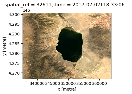
Often, data ingestion involves quickly visualizing your raw data to get a sense that things are proceeding accordingly. As we have created an array with red, blue, and green bands, we can quickly display a natural color image of the lake using the .plot.imshow() function of xarray. We’ll use the robust=True argument because the data values are outside the range of typical RGB images.
da.plot.imshow(robust=True, size=3)
<matplotlib.image.AxesImage at 0x7f4c342a6860>
Now, let’s use hvplot to provide an interactive visualization of the inividual bands in our array.
ds
<xarray.Dataset>
Dimensions: (y: 1128, x: 950)
Coordinates:
* y (y) float64 4.301e+06 4.301e+06 ... 4.267e+06 4.267e+06
* x (x) float64 3.353e+05 3.353e+05 ... 3.637e+05 3.638e+05
spatial_ref int32 32611
time datetime64[ns] 2017-07-02T18:33:06.200763
Data variables:
red (y, x) uint16 dask.array<chunksize=(1128, 950), meta=np.ndarray>
green (y, x) uint16 dask.array<chunksize=(1128, 950), meta=np.ndarray>
blue (y, x) uint16 dask.array<chunksize=(1128, 950), meta=np.ndarray>da.hvplot.image(x="x", y="y", cmap="viridis", aspect=1)
/home/runner/miniconda3/envs/cookbook-dev/lib/python3.10/site-packages/holoviews/core/util.py:1175: FutureWarning: unique with argument that is not not a Series, Index, ExtensionArray, or np.ndarray is deprecated and will raise in a future version.
return pd.unique(values)
Let’s plot the bands as seperate columns by specifying a dimension to expand with col='band'. We can also set rasterize=True to use Datashader (another HoloViz tool) to render large data into a 2D histogram, where every array cell counts the data points falling into that pixel, as set by the resolution of your screen. This is especially important for large and high resolution images that would otherwise cause issues when attempting to render in a browser.
da.hvplot.image(
x="x", y="y", col="band", cmap="viridis", xaxis=False, yaxis=False, colorbar=False, rasterize=True
)
/home/runner/miniconda3/envs/cookbook-dev/lib/python3.10/site-packages/holoviews/core/util.py:1175: FutureWarning: unique with argument that is not not a Series, Index, ExtensionArray, or np.ndarray is deprecated and will raise in a future version.
return pd.unique(values)
/home/runner/miniconda3/envs/cookbook-dev/lib/python3.10/site-packages/dask/dataframe/_pyarrow_compat.py:17: FutureWarning: Minimal version of pyarrow will soon be increased to 14.0.1. You are using 12.0.1. Please consider upgrading.
warnings.warn(
/home/runner/miniconda3/envs/cookbook-dev/lib/python3.10/site-packages/holoviews/core/util.py:1891: FutureWarning: Creating a Groupby object with a length-1 list-like level parameter will yield indexes as tuples in a future version. To keep indexes as scalars, create Groupby objects with a scalar level parameter instead.
groups = ((wrap_tuple(k), group_type(OrderedDict(unpack_group(group, getter)), **kwargs))
Select the zoom tool and zoom in on of the plots to see that all the images are all automatically linked!
Retain Attributes
When working with many image arrays, it’s critical to retain the data properties as xarray attributes:
da.attrs = selected_item.properties
da
<xarray.DataArray (band: 3, y: 1128, x: 950)>
array([[[14691, 14914, 14988, ..., 16283, 16292, 16316],
[14655, 14859, 14969, ..., 16272, 16185, 16079],
[14531, 14699, 14972, ..., 15318, 15526, 14734],
...,
[13804, 13561, 13601, ..., 18311, 18202, 17625],
[13857, 13828, 13858, ..., 19400, 18942, 18551],
[13840, 13786, 13867, ..., 17873, 17917, 18453]],
[[13233, 13402, 13565, ..., 14553, 14658, 14657],
[13291, 13428, 13585, ..., 14590, 14478, 14550],
[13122, 13287, 13601, ..., 13987, 14220, 13571],
...,
[12720, 12552, 12468, ..., 16580, 16411, 15899],
[12704, 12644, 12658, ..., 17351, 16853, 16505],
[12647, 12620, 12698, ..., 15990, 16211, 16686]],
[[11572, 11629, 11723, ..., 12857, 12918, 12946],
[11588, 11655, 11721, ..., 12848, 12792, 12715],
[11510, 11608, 11781, ..., 12371, 12453, 12053],
...,
[11195, 11104, 11045, ..., 14182, 14031, 13716],
[11125, 11061, 11106, ..., 14652, 14284, 14062],
[11059, 11050, 11134, ..., 13756, 13865, 14209]]], dtype=uint16)
Coordinates:
* y (y) float64 4.301e+06 4.301e+06 ... 4.267e+06 4.267e+06
* x (x) float64 3.353e+05 3.353e+05 ... 3.637e+05 3.638e+05
spatial_ref int32 32611
time datetime64[ns] 2017-07-02T18:33:06.200763
* band (band) object 'red' 'green' 'blue'
Attributes: (12/22)
gsd: 30
created: 2022-05-06T17:46:34.110946Z
sci:doi: 10.5066/P9OGBGM6
datetime: 2017-07-02T18:33:06.200763Z
platform: landsat-8
proj:epsg: 32611
... ...
view:sun_azimuth: 125.03739105
landsat:correction: L2SP
view:sun_elevation: 65.85380157
landsat:cloud_cover_land: 0.53
landsat:collection_number: 02
landsat:collection_category: T1Notice that you can now expand the Attributes: dropdown to see the properties of this data.
Set the crs attribute
As the data is in ‘meter’ units from a reference point, we can plot in commonly used longitude, latitude coordinates with .hvplot(geo=True) if our array has a valid coordinate reference system (CRS) attribute. This value is provided from Microsoft Planetary Computer as the proj:epsg property, so we just need to copy it to a new attribute crs so that hvPlot can automatically find it, without us having to further specify anything in our plotting code
Note, this CRS is referenced by an EPSG code that can be accessed from the metadata of our selected catalog search result. We can see more about this dataset’s specific code at EPSG.io/32611. You can also read more about EPSG codes in general in this Coordinate Reference Systems: EPSG codes online book chapter.
da.attrs["crs"] = f"epsg:{selected_item.properties['proj:epsg']}"
da.attrs["crs"]
'epsg:32611'
Now we can use .hvplot(geo=True) to plot in longitude and latitude coordinates. Informing hvPlot that this is geographic data also allows us to overlay data on aligned geographic tiles using the tiles parameter.
da.hvplot.image(
x="x", y="y", cmap="viridis", geo=True, alpha=.9, tiles="ESRI", xlabel="Longitude", ylabel="Latitude", colorbar=False, aspect=1,
)
/home/runner/miniconda3/envs/cookbook-dev/lib/python3.10/site-packages/geoviews/operation/__init__.py:14: HoloviewsDeprecationWarning: 'ResamplingOperation' is deprecated and will be removed in version 1.18, use 'ResampleOperation2D' instead.
from holoviews.operation.datashader import (
/home/runner/miniconda3/envs/cookbook-dev/lib/python3.10/site-packages/holoviews/core/util.py:1175: FutureWarning: unique with argument that is not not a Series, Index, ExtensionArray, or np.ndarray is deprecated and will raise in a future version.
return pd.unique(values)
Summary
The data access approach should adapt to features of the data and your intended analysis. As Landsat data is large and multidimensional, a good approach is to use Microsoft Plantery Computer, pystac-client, and odc-stac together for searching the metadata catalog and lazily loading specific data chunks. Once you have accessed data, visualize it with hvPlot to ensure that it matches your expectations.
What’s next?
Before we proceed to workflow examples, we can explore alternate ways of accessing data and the processing steps that are often utilized.
Resources and References
Authored by Demetris Roumis circa Jan, 2023
Guidance for parts of this notebook was provided by Microsoft in ‘Reading Data from the STAC API’
The image used in the banner is from Microsoft