Data Ingestion - General Purpose Tooling

---

Overview

If the specialized geospatial tools discussed in the previous notebook suit your needs, feel free to proceed to explore a workflow example, such as Spectral Clustering. However, if you’re seeking a tool that is adaptable across a wider range of data types and sources, welcome to this introduction to Intake V2, a general-purpose data ingestion and management library.

Intake is a high-level library designed for data ingestion and management. While the geospatial-specific tooling approach is optimized for satellite data, Intake offers a broader and potentially more flexible approach for multimodal data workflows, characterized by:

• Unified Interface: Abstracts the details of data sources, enabling users to interact with a consistent API regardless of the data’s underlying format.

• Dynamic and Shareable Catalogs: Facilitates the creation and sharing of data catalogs that can be version-controlled, updated, and maintained.

• Extensible: Facilitates the addition of new data sources and formats through its plugin system.

In the following sections, we will guide you through an introduction to various Intake functionalities that simplify data access and enhance both modularity and reproducibility in geospatial workflows.

Prerequisites

Concepts	Importance	Notes
Intro to Landsat	Necessary	Background
Data Ingestion - Geospatial-Specific Tooling	Helpful
Pandas Cookbook	Helpful
xarray Cookbook	Necessary
Intake Quickstart	Helpful
Intake Cookbook	Necessary

• Time to learn: 20 minutes

---

Imports

import intake
import planetary_computer
from pprint import pprint

# Viz
import hvplot.xarray
import panel as pn

pn.extension()

Connecting to Data Sources

To get started, we need to provide a STAC URL (or any other data source URL) to intake, and we can ask intake to recommend some suitable datatypes.

url = "https://planetarycomputer.microsoft.com/api/stac/v1"
data_types = intake.readers.datatypes.recommend(url)
pprint(data_types)

[<class 'intake.readers.datatypes.JSONFile'>,
 <class 'intake.readers.datatypes.STACJSON'>,
 <class 'intake.readers.datatypes.Handle'>,
 <class 'intake.readers.datatypes.CatalogAPI'>,
 <class 'intake.readers.datatypes.TiledService'>]

Selecting the Appropriate Data Type

After identifying the possible data types, we choose the one that best suits our needs. For handling STAC formatted JSON data from our URL, we will proceed with STACJSON.

data_type = intake.datatypes.STACJSON(url)
data_type

STACJSON, {'url': 'https://planetarycomputer.microsoft.com/api/stac/v1', 'storage_options': None, 'metadata': {}}

This object now represents the specific data type we will work with, allowing us to streamline subsequent data operations.

Initializing Data Readers

With the STACJSON data type specified, we explore available methods to read the data.

readers = data_type.possible_readers
pprint(readers)

{'importable': [<class 'intake.readers.catalogs.StacCatalogReader'>,
                <class 'intake.readers.catalogs.StackBands'>,
                <class 'intake.readers.catalogs.StacSearch'>,
                <class 'intake.readers.readers.DaskJSON'>,
                <class 'intake.readers.readers.FileByteReader'>,
                <class 'intake.readers.readers.FileTextReader'>,
                <class 'intake.readers.readers.FileExistsReader'>],
 'not_importable': [<class 'intake.readers.readers.PolarsJSON'>,
                    <class 'intake.readers.readers.RayJSON'>,
                    <class 'intake.readers.readers.AwkwardJSON'>,
                    <class 'intake.readers.readers.DuckJSON'>,
                    <class 'intake.readers.readers.RayBinary'>]}

This output presents us with options that can interpret the STACJSON data format effectively. The StacCatalogReader is probably the most suitable for our use case. We can use it to read the STAC catalog and explore the available contents.

Reading the Catalog

Next, we can access the data catalog through our reader.

reader = intake.catalogs.StacCatalogReader(
    data_type, signer=planetary_computer.sign_inplace
)
reader

StacCatalogReader reader producing intake.readers.entry:Catalog

This reader is now configured to handle interactions with the data catalog.

List Catalog Contents

Once the catalog is accessible, we read() it and then collect each dataset’s description to identify datasets of interest. For our purposes, we will just print the entries that include the word 'landsat'.

stac_cat = reader.read()

description = {}
for data_description in stac_cat.data.values():
    data = data_description.kwargs["data"]
    description[data["id"]] = data["description"]

# Print only keys that include the word 'landsat'
pprint([key for key in description.keys() if 'landsat' in key.lower()])

['landsat-c2-l2', 'landsat-c2-l1']

Detailed Dataset Examination

By examining specific datasets more closely, we understand their content and relevance to our project goals. We can now print the description of the desired landsat IDs.

print("1:", description["landsat-c2-l1"])
print('-------------------------------\n')
print("2:", description["landsat-c2-l2"])

1: Landsat Collection 2 Level-1 data, consisting of quantized and calibrated scaled Digital Numbers (DN) representing the multispectral image data. These [Level-1](https://www.usgs.gov/landsat-missions/landsat-collection-2-level-1-data) data can be [rescaled](https://www.usgs.gov/landsat-missions/using-usgs-landsat-level-1-data-product) to top of atmosphere (TOA) reflectance and/or radiance. Thermal band data can be rescaled to TOA brightness temperature.

This dataset represents the global archive of Level-1 data from [Landsat Collection 2](https://www.usgs.gov/core-science-systems/nli/landsat/landsat-collection-2) acquired by the [Multispectral Scanner System](https://landsat.gsfc.nasa.gov/multispectral-scanner-system/) onboard Landsat 1 through Landsat 5 from July 7, 1972 to January 7, 2013. Images are stored in [cloud-optimized GeoTIFF](https://www.cogeo.org/) format.

-------------------------------

2: Landsat Collection 2 Level-2 [Science Products](https://www.usgs.gov/landsat-missions/landsat-collection-2-level-2-science-products), consisting of atmospherically corrected [surface reflectance](https://www.usgs.gov/landsat-missions/landsat-collection-2-surface-reflectance) and [surface temperature](https://www.usgs.gov/landsat-missions/landsat-collection-2-surface-temperature) image data. Collection 2 Level-2 Science Products are available from August 22, 1982 to present.

This dataset represents the global archive of Level-2 data from [Landsat Collection 2](https://www.usgs.gov/core-science-systems/nli/landsat/landsat-collection-2) acquired by the [Thematic Mapper](https://landsat.gsfc.nasa.gov/thematic-mapper/) onboard Landsat 4 and 5, the [Enhanced Thematic Mapper](https://landsat.gsfc.nasa.gov/the-enhanced-thematic-mapper-plus-etm/) onboard Landsat 7, and the [Operatational Land Imager](https://landsat.gsfc.nasa.gov/satellites/landsat-8/spacecraft-instruments/operational-land-imager/) and [Thermal Infrared Sensor](https://landsat.gsfc.nasa.gov/satellites/landsat-8/spacecraft-instruments/thermal-infrared-sensor/) onboard Landsat 8 and 9. Images are stored in [cloud-optimized GeoTIFF](https://www.cogeo.org/) format.

Selecting and Accessing Data

We want "landsat-c2-l2", so with a chosen dataset, we can now access it directly and view the metadata specific to this dataset - key details that are important for analysis and interpretation. Since the output is long, we’ll utilize the HoloViz Panel library to wrap the output in a scrollable element.

landsat_reader = stac_cat["landsat-c2-l2"]
landsat_metadata = landsat_reader.read().metadata

# View extensive metadata in scrollable block
json_pane = pn.pane.JSON(landsat_metadata, name='Metadata', max_height=400, sizing_mode='stretch_width', depth=-1, theme='light')
scrollable_output = pn.Column(json_pane, height=400, sizing_mode='stretch_width', scroll=True, styles={'background': 'lightgrey'})
scrollable_output

Visual Preview

To get a visual preview of the dataset, particularly to check its quality and relevance, we use the following commands:

landsat_reader["thumbnail"].read()

Accessing Geospatial Data Items

Once we have selected the appropriate dataset, the next step is to access the specific data items. These items typically represent individual data files or collections that are part of the dataset.

The following code retrieves a handle to the ‘geoparquet-items’ from the Landsat dataset, which are optimized for efficient geospatial operations and queries.

landsat_items = landsat_reader["geoparquet-items"]
landsat_items

DaskGeoParquet reader producing dask_geopandas.core:GeoDataFrame

Converting Data for Analysis

To facilitate analysis, the following code selects the last few entries (tail) of the dataset, converts them into a GeoDataFrame, and reads it back into a STAC catalog format. This format is particularly suited for geospatial data and necessary for compatibility with geospatial analysis tools and libraries like Geopandas.

cat = landsat_items.tail(output_instance="geopandas:GeoDataFrame").GeoDataFrameToSTACCatalog.read()

/home/runner/miniconda3/envs/cookbook-dev/lib/python3.10/site-packages/dask/dataframe/_pyarrow_compat.py:17: FutureWarning: Minimal version of pyarrow will soon be increased to 14.0.1. You are using 12.0.1. Please consider upgrading.
  warnings.warn(

/home/runner/miniconda3/envs/cookbook-dev/lib/python3.10/site-packages/geopandas/_compat.py:153: UserWarning: The Shapely GEOS version (3.11.1-CAPI-1.17.1) is incompatible with the GEOS version PyGEOS was compiled with (3.10.4-CAPI-1.16.2). Conversions between both will be slow.
  set_use_pygeos()

Exploring Data Collections

After conversion, we explore the structure of the data collection. Each “item” in this collection corresponds to a set of assets, providing a structured way to access multiple related data files. We’ll simply print the structure of the catalog to understand the available items and their organization.

cat

Catalog
 named datasets: ['LC09_L2SP_098011_20240401_02_T1', 'LC09_L2SP_098012_20240401_02_T1', 'LC09_L2SP_098013_20240401_02_T1', 'LC09_L2SP_098014_20240401_02_T1', 'LC09_L2SP_098015_20240401_02_T1']

Accessing Sub-Collections

To dive deeper into the data, we access a specific sub-collection based on its key. This allows us to focus on a particular geographic area or time period. We’ll select the first item in the catalog for now.

item_key = list(cat.entries.keys())[0]
subcat = cat[item_key].read()
subcat

Catalog
 named datasets: ['ang', 'atran', 'blue', 'cdist', 'coastal', 'drad', 'emis', 'emsd', 'green', 'lwir11', 'mtl.json', 'mtl.txt', 'mtl.xml', 'nir08', 'qa', 'qa_aerosol', 'qa_pixel', 'qa_radsat', 'red', 'rendered_preview', 'swir16', 'swir22', 'tilejson', 'trad', 'urad']

Reading Specific Data Bands

For detailed analysis, especially in remote sensing, accessing specific spectral bands is crucial. Here, we read the red spectral band, which is often used in vegetation analysis and other remote sensing applications.

subcat.red.read()

[<xarray.DataArray (band: 1, y: 8231, x: 8171)>
 [67255501 values with dtype=uint16]
 Coordinates:
   * band         (band) int64 1
   * x            (x) float64 4.854e+05 4.854e+05 ... 7.305e+05 7.305e+05
   * y            (y) float64 7.247e+06 7.247e+06 7.247e+06 ... 7e+06 7e+06 7e+06
     spatial_ref  int64 0
 Attributes:
     AREA_OR_POINT:  Point
     _FillValue:     0
     scale_factor:   1.0
     add_offset:     0.0]

Preparing for Multiband Analysis

To analyze true color imagery, we need to stack multiple spectral bands. Here, we prepare for this by setting up a band-stacking operation. Note, re-signing might be necessary at this point.

catbands = cat[item_key].to_reader(reader="StackBands", bands=["red", "green", "blue"], signer=planetary_computer.sign_inplace)

Loading and Visualizing True Color Imagery

After setting up the band-stacking, we read the multiband data and prepare it for visualization.

data = catbands.read(dim="band")
data

<xarray.DataArray (band: 3, y: 8231, x: 8171)>
array([[[0, 0, 0, ..., 0, 0, 0],
        [0, 0, 0, ..., 0, 0, 0],
        [0, 0, 0, ..., 0, 0, 0],
        ...,
        [0, 0, 0, ..., 0, 0, 0],
        [0, 0, 0, ..., 0, 0, 0],
        [0, 0, 0, ..., 0, 0, 0]],

       [[0, 0, 0, ..., 0, 0, 0],
        [0, 0, 0, ..., 0, 0, 0],
        [0, 0, 0, ..., 0, 0, 0],
        ...,
        [0, 0, 0, ..., 0, 0, 0],
        [0, 0, 0, ..., 0, 0, 0],
        [0, 0, 0, ..., 0, 0, 0]],

       [[0, 0, 0, ..., 0, 0, 0],
        [0, 0, 0, ..., 0, 0, 0],
        [0, 0, 0, ..., 0, 0, 0],
        ...,
        [0, 0, 0, ..., 0, 0, 0],
        [0, 0, 0, ..., 0, 0, 0],
        [0, 0, 0, ..., 0, 0, 0]]], dtype=uint16)
Coordinates:
  * band         (band) int64 1 1 1
  * x            (x) float64 4.854e+05 4.854e+05 ... 7.305e+05 7.305e+05
  * y            (y) float64 7.247e+06 7.247e+06 7.247e+06 ... 7e+06 7e+06 7e+06
    spatial_ref  int64 0
Attributes:
    AREA_OR_POINT:  Point
    _FillValue:     0
    scale_factor:   1.0
    add_offset:     0.0

xarray.DataArray

• band: 3
• y: 8231
• x: 8171

• 0 0 0 0 0 0 0 0 0 0 0 0 0 0 0 0 0 ... 0 0 0 0 0 0 0 0 0 0 0 0 0 0 0 0

  array([[[0, 0, 0, ..., 0, 0, 0],
          [0, 0, 0, ..., 0, 0, 0],
          [0, 0, 0, ..., 0, 0, 0],
          ...,
          [0, 0, 0, ..., 0, 0, 0],
          [0, 0, 0, ..., 0, 0, 0],
          [0, 0, 0, ..., 0, 0, 0]],
  
         [[0, 0, 0, ..., 0, 0, 0],
          [0, 0, 0, ..., 0, 0, 0],
          [0, 0, 0, ..., 0, 0, 0],
          ...,
          [0, 0, 0, ..., 0, 0, 0],
          [0, 0, 0, ..., 0, 0, 0],
          [0, 0, 0, ..., 0, 0, 0]],
  
         [[0, 0, 0, ..., 0, 0, 0],
          [0, 0, 0, ..., 0, 0, 0],
          [0, 0, 0, ..., 0, 0, 0],
          ...,
          [0, 0, 0, ..., 0, 0, 0],
          [0, 0, 0, ..., 0, 0, 0],
          [0, 0, 0, ..., 0, 0, 0]]], dtype=uint16)

• Coordinates: (4)
  • band
    (band)
    int64
    1 1 1

    array([1, 1, 1])

  • x
    (x)
    float64
    4.854e+05 4.854e+05 ... 7.305e+05

    array([485400., 485430., 485460., ..., 730440., 730470., 730500.])

  • y
    (y)
    float64
    7.247e+06 7.247e+06 ... 7e+06 7e+06

    array([7246800., 7246770., 7246740., ..., 6999960., 6999930., 6999900.])

  • spatial_ref
    ()
    int64
    0

    crs_wkt :

    PROJCS["WGS 84 / UTM zone 58N",GEOGCS["WGS 84",DATUM["WGS_1984",SPHEROID["WGS 84",6378137,298.257223563,AUTHORITY["EPSG","7030"]],AUTHORITY["EPSG","6326"]],PRIMEM["Greenwich",0,AUTHORITY["EPSG","8901"]],UNIT["degree",0.0174532925199433,AUTHORITY["EPSG","9122"]],AUTHORITY["EPSG","4326"]],PROJECTION["Transverse_Mercator"],PARAMETER["latitude_of_origin",0],PARAMETER["central_meridian",165],PARAMETER["scale_factor",0.9996],PARAMETER["false_easting",500000],PARAMETER["false_northing",0],UNIT["metre",1,AUTHORITY["EPSG","9001"]],AXIS["Easting",EAST],AXIS["Northing",NORTH],AUTHORITY["EPSG","32658"]]

    semi_major_axis :

    6378137.0

    semi_minor_axis :

    6356752.314245179

    inverse_flattening :

    298.257223563

    reference_ellipsoid_name :

    WGS 84

    longitude_of_prime_meridian :

    0.0

    prime_meridian_name :

    Greenwich

    geographic_crs_name :

    WGS 84

    horizontal_datum_name :

    World Geodetic System 1984

    projected_crs_name :

    WGS 84 / UTM zone 58N

    grid_mapping_name :

    transverse_mercator

    latitude_of_projection_origin :

    0.0

    longitude_of_central_meridian :

    165.0

    false_easting :

    500000.0

    false_northing :

    0.0

    scale_factor_at_central_meridian :

    0.9996

    spatial_ref :

    PROJCS["WGS 84 / UTM zone 58N",GEOGCS["WGS 84",DATUM["WGS_1984",SPHEROID["WGS 84",6378137,298.257223563,AUTHORITY["EPSG","7030"]],AUTHORITY["EPSG","6326"]],PRIMEM["Greenwich",0,AUTHORITY["EPSG","8901"]],UNIT["degree",0.0174532925199433,AUTHORITY["EPSG","9122"]],AUTHORITY["EPSG","4326"]],PROJECTION["Transverse_Mercator"],PARAMETER["latitude_of_origin",0],PARAMETER["central_meridian",165],PARAMETER["scale_factor",0.9996],PARAMETER["false_easting",500000],PARAMETER["false_northing",0],UNIT["metre",1,AUTHORITY["EPSG","9001"]],AXIS["Easting",EAST],AXIS["Northing",NORTH],AUTHORITY["EPSG","32658"]]

    GeoTransform :

    485385.0 30.0 0.0 7246815.0 0.0 -30.0

    array(0)

• Indexes: (3)
  • band
    PandasIndex

    PandasIndex(Int64Index([1, 1, 1], dtype='int64', name='band'))

  • x
    PandasIndex

    PandasIndex(Float64Index([485400.0, 485430.0, 485460.0, 485490.0, 485520.0, 485550.0,
                  485580.0, 485610.0, 485640.0, 485670.0,
                  ...
                  730230.0, 730260.0, 730290.0, 730320.0, 730350.0, 730380.0,
                  730410.0, 730440.0, 730470.0, 730500.0],
                 dtype='float64', name='x', length=8171))

  • y
    PandasIndex

    PandasIndex(Float64Index([7246800.0, 7246770.0, 7246740.0, 7246710.0, 7246680.0, 7246650.0,
                  7246620.0, 7246590.0, 7246560.0, 7246530.0,
                  ...
                  7000170.0, 7000140.0, 7000110.0, 7000080.0, 7000050.0, 7000020.0,
                  6999990.0, 6999960.0, 6999930.0, 6999900.0],
                 dtype='float64', name='y', length=8231))

• Attributes: (4)

  AREA_OR_POINT :

  Point

  _FillValue :

  0

  scale_factor :

  1.0

  add_offset :

  0.0

Visualizing Data

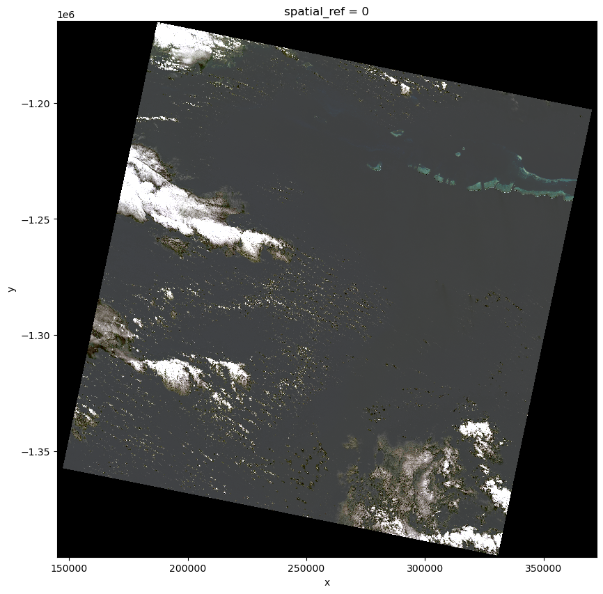
Finally, we visualize the true color imagery. This visualization helps in assessing the quality of the data and the appropriateness of the bands used.

data.plot.imshow(robust=True, figsize=(10, 10))

<matplotlib.image.AxesImage at 0x7f5be1ce5420>

Summary

As earth science data becomes integrated with other types of data, a powerful approach is to utilize a general purpose set of tools, including Intake and Xarray. Once you have accessed data, visualize it with hvPlot to ensure that it matches your expectations.

What’s next?

Now that we know how to access the data, it’s time to proceed to analysis, where we will explore a some simple machine learning approaches.

Resources and references

Authored by Demetris Roumis and Andrew Huang circa April, 2024, with guidance from Martin Durant.

The banner image is a mashup of a Landsat 8 image from NASA and the Intake logo.