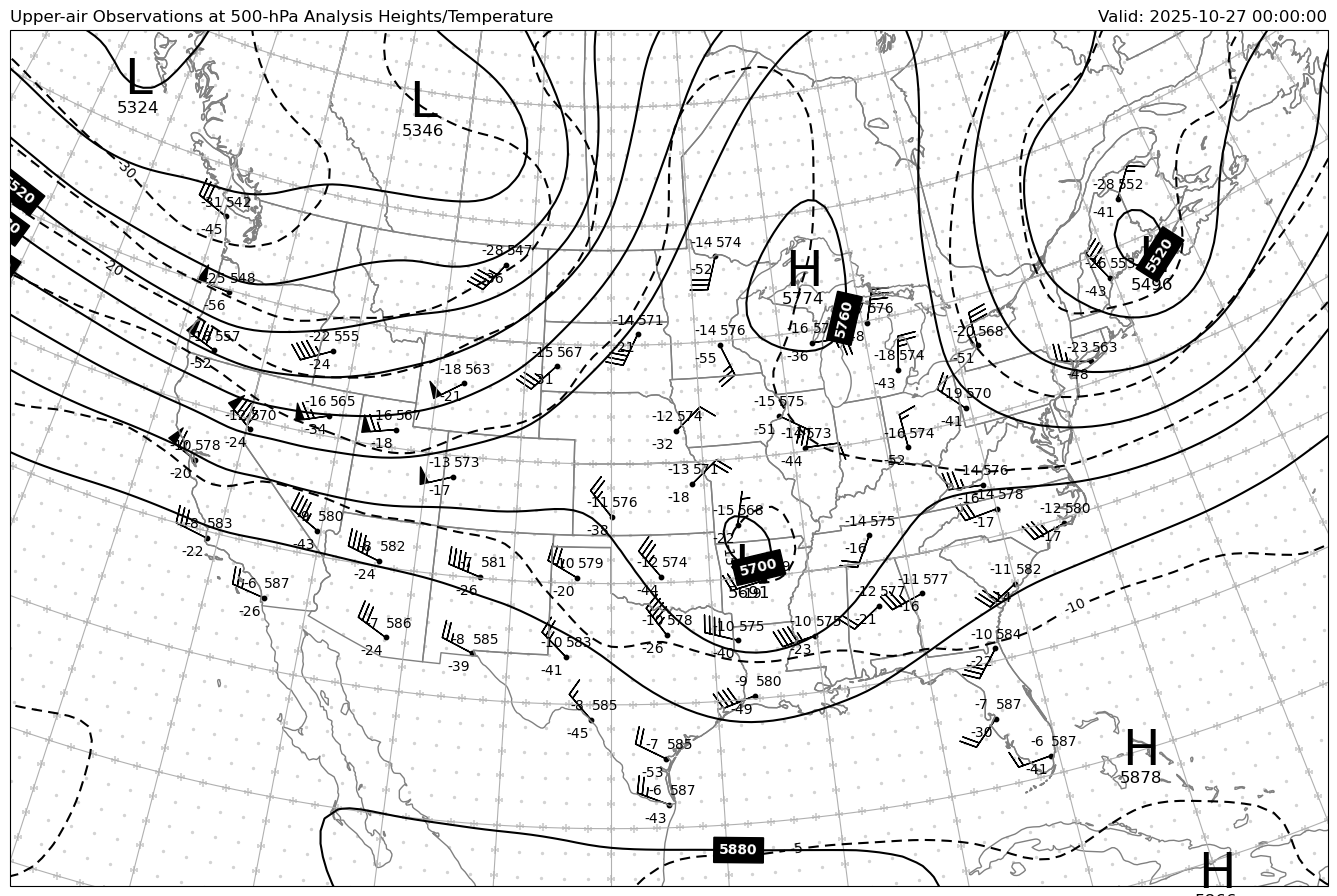
This example replicates the traditional DIFAX images for upper-level observations.
By: Kevin Goebbert
Observation data comes from Iowa State Archive, accessed through the Siphon package. Contour data comes from the GFS 0.5 degree analysis. Classic upper-level data of Geopotential Height and Temperature are plotted.
import urllib.request

from datetime import datetime, timedelta, UTC

import cartopy.crs as ccrs
import cartopy.feature as cfeature
import matplotlib.pyplot as plt
from matplotlib.ticker import FixedLocator
import metpy.calc as mpcalc
import numpy as np
import xarray as xr

from metpy.io import add_station_lat_lon
from metpy.calc import find_peaks
from metpy.plots import scattertext, StationPlot
from metpy.units import units
from siphon.simplewebservice.iastate import IAStateUpperAir
Observation Data
Set a date and time for upper-air observations (should only be 00 or 12 UTC for the hour).
Request all data from Iowa State using the Siphon package. The result is a pandas DataFrame containing all of the sounding data from all available stations.
# Set date for desired UPA data
today = datetime.now(UTC)

# Go back one day to ensure data availability
date = datetime(today.year, today.month, today.day, 0) - timedelta(days=1)

# Request data using Siphon request for data from Iowa State Archive
data = IAStateUpperAir.request_all_data(date)
Subset Observational Data
From the request above will give all levels from all radisonde sites available through the service. For plotting a pressure surface map there is only need to have the data from that level. Below the data is subset and a few parameters set based on the level chosen. Additionally, the station information is obtained and latitude and longitude data is added to the DataFrame.
level = 500

if (level == 925) | (level == 850) | (level == 700):
    cint = 30
    def hght_format(v): return format(v, '.0f')[1:]
elif level == 500:
    cint = 60
    def hght_format(v): return format(v, '.0f')[:3]
elif level == 300:
    cint = 120
    def hght_format(v): return format(v, '.0f')[:3]
elif level < 300:
    cint = 120
    def hght_format(v): return format(v, '.0f')[1:4]

# Create subset of all data for a given level
data_subset = data.pressure == level
df = data[data_subset]

# Get station lat/lon from look-up file; add to Dataframe
df = add_station_lat_lon(df)
Downloading file 'sfstns.tbl' from 'https://github.com/Unidata/MetPy/raw/v1.7.1/staticdata/sfstns.tbl' to '/home/runner/.cache/metpy/v1.7.1'.
Downloading file 'master.txt' from 'https://github.com/Unidata/MetPy/raw/v1.7.1/staticdata/master.txt' to '/home/runner/.cache/metpy/v1.7.1'.
Downloading file 'stations.txt' from 'https://github.com/Unidata/MetPy/raw/v1.7.1/staticdata/stations.txt' to '/home/runner/.cache/metpy/v1.7.1'.
Downloading file 'airport-codes.csv' from 'https://github.com/Unidata/MetPy/raw/v1.7.1/staticdata/airport-codes.csv' to '/home/runner/.cache/metpy/v1.7.1'.
Gridded Data
Obtain GFS gridded output for contour plotting. Specifically, geopotential height and temperature data for the given level and subset for over North America. Data are smoothed for aesthetic reasons.
# Get GFS data and subset to North America for Geopotential Height and Temperature
ds = xr.open_dataset('https://thredds.ucar.edu/thredds/dodsC/grib/NCEP/GFS/Global_0p5deg_ana/'
                     'GFS_Global_0p5deg_ana_{0:%Y%m%d}_{0:%H}00.grib2'.format(
                         date)).metpy.parse_cf()

# Geopotential height
hght = ds.Geopotential_height_isobaric.metpy.sel(
    vertical=level*units.hPa, time=date, lat=slice(70, 15), lon=slice(360-145, 360-50))

# Temperature
tmpk = ds.Temperature_isobaric.metpy.sel(
    vertical=level*units.hPa, time=date, lat=slice(70, 15), lon=slice(360-145, 360-50))
New in MetPy v1.7, we can use metpy
# Find the location of local max/min geopotential heights
H_y, H_x = find_peaks(hght, iqr_ratio=4)
L_y, L_x = find_peaks(hght, maxima=False, iqr_ratio=4)

# Smooth our fields for the chart
smooth_hght = mpcalc.smooth_n_point(hght, 9, 10)
smooth_tmpc = (mpcalc.smooth_n_point(tmpk, 9, 10)).metpy.convert_units('degC')
Create DIFAX Replication
Plot the observational data and contours on a Lambert Conformal map and add features that resemble the historic DIFAX maps.
# Set up map coordinate reference system
mapcrs = ccrs.LambertConformal(
    central_latitude=45, central_longitude=-100, standard_parallels=(30, 60))

# Set up station locations for plotting observations
point_locs = mapcrs.transform_points(
    ccrs.PlateCarree(), df['longitude'].values, df['latitude'].values)

# Start figure and set graphics extent
fig = plt.figure(1, figsize=(17, 15))
ax = plt.subplot(111, projection=mapcrs)
ax.set_extent([-125, -70, 20, 55])

# Add map features for geographic reference
ax.add_feature(cfeature.COASTLINE.with_scale('50m'), edgecolor='grey')
ax.add_feature(cfeature.LAND.with_scale('50m'), facecolor='white')
ax.add_feature(cfeature.STATES.with_scale('50m'), edgecolor='grey')

# Plot plus signs every degree lat/lon
plus_lat = []
plus_lon = []
other_lat = []
other_lon = []

for x in hght.lon.values[::2]:
    for y in hght.lat.values[::2]:
        if (x % 5 == 0) | (y % 5 == 0):
            plus_lon.append(x)
            plus_lat.append(y)
        else:
            other_lon.append(x)
            other_lat.append(y)
ax.scatter(other_lon, other_lat, s=2, marker='o',
           transform=ccrs.PlateCarree(), color='lightgrey', zorder=-1)
ax.scatter(plus_lon, plus_lat, s=30, marker='+', transform=ccrs.PlateCarree(),
           color='lightgrey')

# Add gridlines for every 5 degree lat/lon
ax.gridlines(linestyle='solid', ylocs=range(15, 71, 5), xlocs=range(-150, -49, 5))

# Start the station plot by specifying the axes to draw on, as well as the
# lon/lat of the stations (with transform). We also the fontsize to 10 pt.
stationplot = StationPlot(ax, df['longitude'].values, df['latitude'].values, clip_on=True,
                          transform=ccrs.PlateCarree(), fontsize=10)

# Plot the temperature and dew point to the upper and lower left, respectively, of
# the center point.
stationplot.plot_parameter('NW', df['temperature'], color='black')
stationplot.plot_parameter('SW', df['dewpoint'], color='black')

# A more complex example uses a custom formatter to control how the geopotential height
# values are plotted. This is set in an earlier if-statement to work appropriate for
# different levels.
stationplot.plot_parameter('NE', df['height'], formatter=hght_format)

# Add wind barbs
stationplot.plot_barb(df['u_wind'], df['v_wind'], length=7, pivot='tip')

# Plot Solid Contours of Geopotential Height
cs = ax.contour(hght.lon, hght.lat, smooth_hght,
                range(0, 20000, cint), colors='black', transform=ccrs.PlateCarree())
clabels = plt.clabel(cs, fmt='%d', colors='white', inline_spacing=5, use_clabeltext=True)

# Contour labels with black boxes and white text
for t in cs.labelTexts:
    t.set_bbox({'facecolor': 'black', 'pad': 4})
    t.set_fontweight('heavy')

# Plot Dashed Contours of Temperature
cs2 = ax.contour(hght.lon, hght.lat, smooth_tmpc, range(-60, 51, 5),
                 colors='black', transform=ccrs.PlateCarree())
clabels = plt.clabel(cs2, fmt='%d', colors='black', inline_spacing=5, use_clabeltext=True)

# Set longer dashes than default
cs2.set(dashes=(0, (5.0, 3.0)))

# Contour labels with black boxes and white text
for t in cs.labelTexts:
    t.set_bbox({'facecolor': 'black', 'pad': 4})
    t.set_fontweight('heavy')

# Plot filled circles for Radiosonde Obs
ax.scatter(df['longitude'].values, df['latitude'].values, s=10,
           marker='o', color='black', transform=ccrs.PlateCarree())

# Plot H/L symbols with metpy.plots.scattertext
# and their corresponding height values 20 pts below the symbol
scattertext(ax, hght.metpy.x[H_x], hght.metpy.y[H_y], 'H',
            size=36, color='black', transform=ccrs.PlateCarree())
scattertext(ax, hght.metpy.x[H_x], hght.metpy.y[H_y], hght.values[H_y, H_x],
            size=12, color='black', formatter='.0f', loc=(0, -20), transform=ccrs.PlateCarree())

scattertext(ax, hght.metpy.x[L_x], hght.metpy.y[L_y], 'L',
            size=36, color='black', transform=ccrs.PlateCarree())
scattertext(ax, hght.metpy.x[L_x], hght.metpy.y[L_y], hght.values[L_y, L_x],
            size=12, color='black', formatter='.0f', loc=(0, -20), transform=ccrs.PlateCarree())

# Add titles
plt.title(f'Upper-air Observations at {level}-hPa Analysis Heights/Temperature',
          loc='left')
plt.title(f'Valid: {date}', loc='right');