![]()


Basic Visualization using matplotlib and Cartopy
Overview
A team at Google Research & Cloud are making parts of the ECMWF Reanalysis version 5 (aka ERA-5) accessible in a Analysis Ready, Cloud Optimized (aka ARCO) format.
In this notebook, we will do the following:
Access the ERA-5 ARCO catalog
Select a particular dataset and variable from the catalog
Convert the data from Gaussian to Cartesian coordinates
Plot a map of sea-level pressure at a specific date and time using Matplotlib and Cartopy.
Prerequisites
Time to learn: 30 minutes
Imports
import fsspec
import xarray as xr
import matplotlib.pyplot as plt
import cartopy.crs as ccrs
import cartopy.feature as cfeature
import scipy.spatial
import numpy as np
import cf_xarray as cfxr
Access the ARCO ERA-5 catalog on Google Cloud
Test bucket access with fsspec
fs = fsspec.filesystem('gs')
fs.ls('gs://gcp-public-data-arco-era5/co')
['gcp-public-data-arco-era5/co/model-level-moisture.zarr',
 'gcp-public-data-arco-era5/co/model-level-moisture.zarr-v2',
 'gcp-public-data-arco-era5/co/model-level-wind.zarr',
 'gcp-public-data-arco-era5/co/model-level-wind.zarr-v2',
 'gcp-public-data-arco-era5/co/single-level-forecast.zarr',
 'gcp-public-data-arco-era5/co/single-level-forecast.zarr-v2',
 'gcp-public-data-arco-era5/co/single-level-reanalysis.zarr',
 'gcp-public-data-arco-era5/co/single-level-reanalysis.zarr-v2',
 'gcp-public-data-arco-era5/co/single-level-surface.zarr',
 'gcp-public-data-arco-era5/co/single-level-surface.zarr-v2']
Let’s open the single-level-reanalysis Zarr file.
reanalysis = xr.open_zarr(
    'gs://gcp-public-data-arco-era5/co/single-level-reanalysis.zarr',
    chunks={'time': 48},
    consolidated=True,
)
print(f'size: {reanalysis.nbytes / (1024 ** 4)} TB')
size: 28.02835009436967 TB
That’s … a big file! But Xarray is just lazy loading the data. We can access the dataset’s metadata:
reanalysis
<xarray.Dataset> Size: 31TB
Dimensions:              (time: 374016, values: 542080)
Coordinates:
    depthBelowLandLayer  float64 8B ...
    entireAtmosphere     float64 8B ...
    latitude             (values) float64 4MB dask.array<chunksize=(542080,), meta=np.ndarray>
    longitude            (values) float64 4MB dask.array<chunksize=(542080,), meta=np.ndarray>
    number               int64 8B ...
    step                 timedelta64[ns] 8B ...
    surface              float64 8B ...
  * time                 (time) datetime64[ns] 3MB 1979-01-01 ... 2021-08-31T...
    valid_time           (time) datetime64[ns] 3MB dask.array<chunksize=(48,), meta=np.ndarray>
Dimensions without coordinates: values
Data variables: (12/38)
    cape                 (time, values) float32 811GB dask.array<chunksize=(48, 542080), meta=np.ndarray>
    d2m                  (time, values) float32 811GB dask.array<chunksize=(48, 542080), meta=np.ndarray>
    hcc                  (time, values) float32 811GB dask.array<chunksize=(48, 542080), meta=np.ndarray>
    istl1                (time, values) float32 811GB dask.array<chunksize=(48, 542080), meta=np.ndarray>
    istl2                (time, values) float32 811GB dask.array<chunksize=(48, 542080), meta=np.ndarray>
    istl3                (time, values) float32 811GB dask.array<chunksize=(48, 542080), meta=np.ndarray>
    ...                   ...
    tsn                  (time, values) float32 811GB dask.array<chunksize=(48, 542080), meta=np.ndarray>
    u10                  (time, values) float32 811GB dask.array<chunksize=(48, 542080), meta=np.ndarray>
    u100                 (time, values) float32 811GB dask.array<chunksize=(48, 542080), meta=np.ndarray>
    v10                  (time, values) float32 811GB dask.array<chunksize=(48, 542080), meta=np.ndarray>
    v100                 (time, values) float32 811GB dask.array<chunksize=(48, 542080), meta=np.ndarray>
    z                    (time, values) float32 811GB dask.array<chunksize=(48, 542080), meta=np.ndarray>
Attributes:
    Conventions:               CF-1.7
    GRIB_centre:               ecmf
    GRIB_centreDescription:    European Centre for Medium-Range Weather Forec...
    GRIB_edition:              1
    GRIB_subCentre:            0
    history:                   2022-09-23T18:56 GRIB to CDM+CF via cfgrib-0.9...
    institution:               European Centre for Medium-Range Weather Forec...
    pangeo-forge:inputs_hash:  5f4378143e9f42402424280b63472752da3aa79179b53b...
    pangeo-forge:recipe_hash:  0c3415923e347ce9dac9dc5c6d209525f4d45d799bd25b...
pangeo-forge:version: 0.9.1- time: 374016
- values: 542080
- depthBelowLandLayer()float64...
- long_name :
- soil depth
- positive :
- down
- standard_name :
- depth
- units :
- m
[1 values with dtype=float64]
- entireAtmosphere()float64...
- long_name :
- original GRIB coordinate for key: level(entireAtmosphere)
- units :
- 1
[1 values with dtype=float64]
- latitude(values)float64dask.array<chunksize=(542080,), meta=np.ndarray>
- long_name :
- latitude
- standard_name :
- latitude
- units :
- degrees_north
Array Chunk Bytes 4.14 MiB 4.14 MiB Shape (542080,) (542080,) Dask graph 1 chunks in 2 graph layers Data type float64 numpy.ndarray - longitude(values)float64dask.array<chunksize=(542080,), meta=np.ndarray>
- long_name :
- longitude
- standard_name :
- longitude
- units :
- degrees_east
Array Chunk Bytes 4.14 MiB 4.14 MiB Shape (542080,) (542080,) Dask graph 1 chunks in 2 graph layers Data type float64 numpy.ndarray - number()int64...
- long_name :
- ensemble member numerical id
- standard_name :
- realization
- units :
- 1
[1 values with dtype=int64]
- step()timedelta64[ns]...
- long_name :
- time since forecast_reference_time
- standard_name :
- forecast_period
[1 values with dtype=timedelta64[ns]]
- surface()float64...
- long_name :
- original GRIB coordinate for key: level(surface)
- units :
- 1
[1 values with dtype=float64]
- time(time)datetime64[ns]1979-01-01 ... 2021-08-31T23:00:00
- long_name :
- initial time of forecast
- standard_name :
- forecast_reference_time
array(['1979-01-01T00:00:00.000000000', '1979-01-01T01:00:00.000000000', '1979-01-01T02:00:00.000000000', ..., '2021-08-31T21:00:00.000000000', '2021-08-31T22:00:00.000000000', '2021-08-31T23:00:00.000000000'], dtype='datetime64[ns]') - valid_time(time)datetime64[ns]dask.array<chunksize=(48,), meta=np.ndarray>
- long_name :
- time
- standard_name :
- time
Array Chunk Bytes 2.85 MiB 384 B Shape (374016,) (48,) Dask graph 7792 chunks in 2 graph layers Data type datetime64[ns] numpy.ndarray
- cape(time, values)float32dask.array<chunksize=(48, 542080), meta=np.ndarray>
- GRIB_N :
- 320
- GRIB_NV :
- 0
- GRIB_cfName :
- unknown
- GRIB_cfVarName :
- cape
- GRIB_dataType :
- an
- GRIB_gridDefinitionDescription :
- Gaussian Latitude/Longitude Grid
- GRIB_gridType :
- reduced_gg
- GRIB_latitudeOfFirstGridPointInDegrees :
- 89.784
- GRIB_latitudeOfLastGridPointInDegrees :
- -89.784
- GRIB_longitudeOfFirstGridPointInDegrees :
- 0.0
- GRIB_longitudeOfLastGridPointInDegrees :
- 359.718
- GRIB_missingValue :
- 9999
- GRIB_name :
- Convective available potential energy
- GRIB_numberOfPoints :
- 542080
- GRIB_paramId :
- 59
- GRIB_pl :
- [18, 25, 36, 40, 45, 50, 60, 64, 72, 72, 75, 81, 90, 96, 100, 108, 120, 120, 125, 135, 144, 144, 150, 160, 180, 180, 180, 192, 192, 200, 216, 216, 216, 225, 240, 240, 240, 250, 256, 270, 270, 288, 288, 288, 300, 300, 320, 320, 320, 324, 360, 360, 360, 360, 360, 360, 375, 375, 384, 384, 400, 400, 405, 432, 432, 432, 432, 450, 450, 450, 480, 480, 480, 480, 480, 486, 500, 500, 500, 512, 512, 540, 540, 540, 540, 540, 576, 576, 576, 576, 576, 576, 600, 600, 600, 600, 640, 640, 640, 640, 640, 640, 640, 648, 648, 675, 675, 675, 675, 720, 720, 720, 720, 720, 720, 720, 720, 720, 729, 750, 750, 750, 750, 768, 768, 768, 768, 800, 800, 800, 800, 800, 800, 810, 810, 864, 864, 864, 864, 864, 864, 864, 864, 864, 864, 864, 900, 900, 900, 900, 900, 900, 900, 900, 960, 960, 960, 960, 960, 960, 960, 960, 960, 960, 960, 960, 960, 960, 972, 972, 1000, 1000, 1000, 1000, 1000, 1000, 1000, 1000, 1024, 1024, 1024, 1024, 1024, 1024, 1080, 1080, 1080, 1080, 1080, 1080, 1080, 1080, 1080, 1080, 1080, 1080, 1080, 1080, 1125, 1125, 1125, 1125, 1125, 1125, 1125, 1125, 1125, 1125, 1125, 1125, 1125, 1125, 1152, 1152, 1152, 1152, 1152, 1152, 1152, 1152, 1152, 1200, 1200, 1200, 1200, 1200, 1200, 1200, 1200, 1200, 1200, 1200, 1200, 1200, 1200, 1200, 1200, 1200, 1200, 1215, 1215, 1215, 1215, 1215, 1215, 1215, 1280, 1280, 1280, 1280, 1280, 1280, 1280, 1280, 1280, 1280, 1280, 1280, 1280, 1280, 1280, 1280, 1280, 1280, 1280, 1280, 1280, 1280, 1280, 1280, 1280, 1280, 1280, 1280, 1280, 1280, 1280, 1280, 1280, 1280, 1280, 1280, 1280, 1280, 1280, 1280, 1280, 1280, 1280, 1280, 1280, 1280, 1280, 1280, 1280, 1280, 1280, 1280, 1280, 1280, 1280, 1280, 1280, 1280, 1280, 1280, 1280, 1280, 1280, 1280, 1280, 1280, 1280, 1280, 1280, 1280, 1280, 1280, 1280, 1280, 1280, 1280, 1280, 1280, 1280, 1280, 1280, 1280, 1280, 1280, 1280, 1280, 1280, 1280, 1280, 1280, 1280, 1280, 1280, 1280, 1280, 1280, 1280, 1280, 1280, 1280, 1280, 1280, 1280, 1280, 1280, 1280, 1280, 1280, 1280, 1280, 1280, 1280, 1280, 1280, 1280, 1280, 1280, 1280, 1280, 1280, 1280, 1280, 1280, 1280, 1280, 1280, 1280, 1280, 1280, 1280, 1280, 1280, 1280, 1280, 1280, 1280, 1280, 1280, 1280, 1280, 1280, 1280, 1280, 1280, 1280, 1280, 1280, 1280, 1215, 1215, 1215, 1215, 1215, 1215, 1215, 1200, 1200, 1200, 1200, 1200, 1200, 1200, 1200, 1200, 1200, 1200, 1200, 1200, 1200, 1200, 1200, 1200, 1200, 1152, 1152, 1152, 1152, 1152, 1152, 1152, 1152, 1152, 1125, 1125, 1125, 1125, 1125, 1125, 1125, 1125, 1125, 1125, 1125, 1125, 1125, 1125, 1080, 1080, 1080, 1080, 1080, 1080, 1080, 1080, 1080, 1080, 1080, 1080, 1080, 1080, 1024, 1024, 1024, 1024, 1024, 1024, 1000, 1000, 1000, 1000, 1000, 1000, 1000, 1000, 972, 972, 960, 960, 960, 960, 960, 960, 960, 960, 960, 960, 960, 960, 960, 960, 900, 900, 900, 900, 900, 900, 900, 900, 864, 864, 864, 864, 864, 864, 864, 864, 864, 864, 864, 810, 810, 800, 800, 800, 800, 800, 800, 768, 768, 768, 768, 750, 750, 750, 750, 729, 720, 720, 720, 720, 720, 720, 720, 720, 720, 675, 675, 675, 675, 648, 648, 640, 640, 640, 640, 640, 640, 640, 600, 600, 600, 600, 576, 576, 576, 576, 576, 576, 540, 540, 540, 540, 540, 512, 512, 500, 500, 500, 486, 480, 480, 480, 480, 480, 450, 450, 450, 432, 432, 432, 432, 405, 400, 400, 384, 384, 375, 375, 360, 360, 360, 360, 360, 360, 324, 320, 320, 320, 300, 300, 288, 288, 288, 270, 270, 256, 250, 240, 240, 240, 225, 216, 216, 216, 200, 192, 192, 180, 180, 180, 160, 150, 144, 144, 135, 125, 120, 120, 108, 100, 96, 90, 81, 75, 72, 72, 64, 60, 50, 45, 40, 36, 25, 18]
- GRIB_shortName :
- cape
- GRIB_stepType :
- instant
- GRIB_stepUnits :
- 1
- GRIB_totalNumber :
- 0
- GRIB_typeOfLevel :
- surface
- GRIB_units :
- J kg**-1
- long_name :
- Convective available potential energy
- standard_name :
- unknown
- units :
- J kg**-1
Array Chunk Bytes 755.29 GiB 99.26 MiB Shape (374016, 542080) (48, 542080) Dask graph 7792 chunks in 2 graph layers Data type float32 numpy.ndarray - d2m(time, values)float32dask.array<chunksize=(48, 542080), meta=np.ndarray>
- GRIB_N :
- 320
- GRIB_NV :
- 0
- GRIB_cfName :
- unknown
- GRIB_cfVarName :
- d2m
- GRIB_dataType :
- an
- GRIB_gridDefinitionDescription :
- Gaussian Latitude/Longitude Grid
- GRIB_gridType :
- reduced_gg
- GRIB_latitudeOfFirstGridPointInDegrees :
- 89.784
- GRIB_latitudeOfLastGridPointInDegrees :
- -89.784
- GRIB_longitudeOfFirstGridPointInDegrees :
- 0.0
- GRIB_longitudeOfLastGridPointInDegrees :
- 359.718
- GRIB_missingValue :
- 9999
- GRIB_name :
- 2 metre dewpoint temperature
- GRIB_numberOfPoints :
- 542080
- GRIB_paramId :
- 168
- GRIB_pl :
- [18, 25, 36, 40, 45, 50, 60, 64, 72, 72, 75, 81, 90, 96, 100, 108, 120, 120, 125, 135, 144, 144, 150, 160, 180, 180, 180, 192, 192, 200, 216, 216, 216, 225, 240, 240, 240, 250, 256, 270, 270, 288, 288, 288, 300, 300, 320, 320, 320, 324, 360, 360, 360, 360, 360, 360, 375, 375, 384, 384, 400, 400, 405, 432, 432, 432, 432, 450, 450, 450, 480, 480, 480, 480, 480, 486, 500, 500, 500, 512, 512, 540, 540, 540, 540, 540, 576, 576, 576, 576, 576, 576, 600, 600, 600, 600, 640, 640, 640, 640, 640, 640, 640, 648, 648, 675, 675, 675, 675, 720, 720, 720, 720, 720, 720, 720, 720, 720, 729, 750, 750, 750, 750, 768, 768, 768, 768, 800, 800, 800, 800, 800, 800, 810, 810, 864, 864, 864, 864, 864, 864, 864, 864, 864, 864, 864, 900, 900, 900, 900, 900, 900, 900, 900, 960, 960, 960, 960, 960, 960, 960, 960, 960, 960, 960, 960, 960, 960, 972, 972, 1000, 1000, 1000, 1000, 1000, 1000, 1000, 1000, 1024, 1024, 1024, 1024, 1024, 1024, 1080, 1080, 1080, 1080, 1080, 1080, 1080, 1080, 1080, 1080, 1080, 1080, 1080, 1080, 1125, 1125, 1125, 1125, 1125, 1125, 1125, 1125, 1125, 1125, 1125, 1125, 1125, 1125, 1152, 1152, 1152, 1152, 1152, 1152, 1152, 1152, 1152, 1200, 1200, 1200, 1200, 1200, 1200, 1200, 1200, 1200, 1200, 1200, 1200, 1200, 1200, 1200, 1200, 1200, 1200, 1215, 1215, 1215, 1215, 1215, 1215, 1215, 1280, 1280, 1280, 1280, 1280, 1280, 1280, 1280, 1280, 1280, 1280, 1280, 1280, 1280, 1280, 1280, 1280, 1280, 1280, 1280, 1280, 1280, 1280, 1280, 1280, 1280, 1280, 1280, 1280, 1280, 1280, 1280, 1280, 1280, 1280, 1280, 1280, 1280, 1280, 1280, 1280, 1280, 1280, 1280, 1280, 1280, 1280, 1280, 1280, 1280, 1280, 1280, 1280, 1280, 1280, 1280, 1280, 1280, 1280, 1280, 1280, 1280, 1280, 1280, 1280, 1280, 1280, 1280, 1280, 1280, 1280, 1280, 1280, 1280, 1280, 1280, 1280, 1280, 1280, 1280, 1280, 1280, 1280, 1280, 1280, 1280, 1280, 1280, 1280, 1280, 1280, 1280, 1280, 1280, 1280, 1280, 1280, 1280, 1280, 1280, 1280, 1280, 1280, 1280, 1280, 1280, 1280, 1280, 1280, 1280, 1280, 1280, 1280, 1280, 1280, 1280, 1280, 1280, 1280, 1280, 1280, 1280, 1280, 1280, 1280, 1280, 1280, 1280, 1280, 1280, 1280, 1280, 1280, 1280, 1280, 1280, 1280, 1280, 1280, 1280, 1280, 1280, 1280, 1280, 1280, 1280, 1280, 1280, 1215, 1215, 1215, 1215, 1215, 1215, 1215, 1200, 1200, 1200, 1200, 1200, 1200, 1200, 1200, 1200, 1200, 1200, 1200, 1200, 1200, 1200, 1200, 1200, 1200, 1152, 1152, 1152, 1152, 1152, 1152, 1152, 1152, 1152, 1125, 1125, 1125, 1125, 1125, 1125, 1125, 1125, 1125, 1125, 1125, 1125, 1125, 1125, 1080, 1080, 1080, 1080, 1080, 1080, 1080, 1080, 1080, 1080, 1080, 1080, 1080, 1080, 1024, 1024, 1024, 1024, 1024, 1024, 1000, 1000, 1000, 1000, 1000, 1000, 1000, 1000, 972, 972, 960, 960, 960, 960, 960, 960, 960, 960, 960, 960, 960, 960, 960, 960, 900, 900, 900, 900, 900, 900, 900, 900, 864, 864, 864, 864, 864, 864, 864, 864, 864, 864, 864, 810, 810, 800, 800, 800, 800, 800, 800, 768, 768, 768, 768, 750, 750, 750, 750, 729, 720, 720, 720, 720, 720, 720, 720, 720, 720, 675, 675, 675, 675, 648, 648, 640, 640, 640, 640, 640, 640, 640, 600, 600, 600, 600, 576, 576, 576, 576, 576, 576, 540, 540, 540, 540, 540, 512, 512, 500, 500, 500, 486, 480, 480, 480, 480, 480, 450, 450, 450, 432, 432, 432, 432, 405, 400, 400, 384, 384, 375, 375, 360, 360, 360, 360, 360, 360, 324, 320, 320, 320, 300, 300, 288, 288, 288, 270, 270, 256, 250, 240, 240, 240, 225, 216, 216, 216, 200, 192, 192, 180, 180, 180, 160, 150, 144, 144, 135, 125, 120, 120, 108, 100, 96, 90, 81, 75, 72, 72, 64, 60, 50, 45, 40, 36, 25, 18]
- GRIB_shortName :
- 2d
- GRIB_stepType :
- instant
- GRIB_stepUnits :
- 1
- GRIB_totalNumber :
- 0
- GRIB_typeOfLevel :
- surface
- GRIB_units :
- K
- long_name :
- 2 metre dewpoint temperature
- standard_name :
- unknown
- units :
- K
Array Chunk Bytes 755.29 GiB 99.26 MiB Shape (374016, 542080) (48, 542080) Dask graph 7792 chunks in 2 graph layers Data type float32 numpy.ndarray - hcc(time, values)float32dask.array<chunksize=(48, 542080), meta=np.ndarray>
- GRIB_N :
- 320
- GRIB_NV :
- 0
- GRIB_cfName :
- unknown
- GRIB_cfVarName :
- hcc
- GRIB_dataType :
- an
- GRIB_gridDefinitionDescription :
- Gaussian Latitude/Longitude Grid
- GRIB_gridType :
- reduced_gg
- GRIB_latitudeOfFirstGridPointInDegrees :
- 89.784
- GRIB_latitudeOfLastGridPointInDegrees :
- -89.784
- GRIB_longitudeOfFirstGridPointInDegrees :
- 0.0
- GRIB_longitudeOfLastGridPointInDegrees :
- 359.718
- GRIB_missingValue :
- 9999
- GRIB_name :
- High cloud cover
- GRIB_numberOfPoints :
- 542080
- GRIB_paramId :
- 188
- GRIB_pl :
- [18, 25, 36, 40, 45, 50, 60, 64, 72, 72, 75, 81, 90, 96, 100, 108, 120, 120, 125, 135, 144, 144, 150, 160, 180, 180, 180, 192, 192, 200, 216, 216, 216, 225, 240, 240, 240, 250, 256, 270, 270, 288, 288, 288, 300, 300, 320, 320, 320, 324, 360, 360, 360, 360, 360, 360, 375, 375, 384, 384, 400, 400, 405, 432, 432, 432, 432, 450, 450, 450, 480, 480, 480, 480, 480, 486, 500, 500, 500, 512, 512, 540, 540, 540, 540, 540, 576, 576, 576, 576, 576, 576, 600, 600, 600, 600, 640, 640, 640, 640, 640, 640, 640, 648, 648, 675, 675, 675, 675, 720, 720, 720, 720, 720, 720, 720, 720, 720, 729, 750, 750, 750, 750, 768, 768, 768, 768, 800, 800, 800, 800, 800, 800, 810, 810, 864, 864, 864, 864, 864, 864, 864, 864, 864, 864, 864, 900, 900, 900, 900, 900, 900, 900, 900, 960, 960, 960, 960, 960, 960, 960, 960, 960, 960, 960, 960, 960, 960, 972, 972, 1000, 1000, 1000, 1000, 1000, 1000, 1000, 1000, 1024, 1024, 1024, 1024, 1024, 1024, 1080, 1080, 1080, 1080, 1080, 1080, 1080, 1080, 1080, 1080, 1080, 1080, 1080, 1080, 1125, 1125, 1125, 1125, 1125, 1125, 1125, 1125, 1125, 1125, 1125, 1125, 1125, 1125, 1152, 1152, 1152, 1152, 1152, 1152, 1152, 1152, 1152, 1200, 1200, 1200, 1200, 1200, 1200, 1200, 1200, 1200, 1200, 1200, 1200, 1200, 1200, 1200, 1200, 1200, 1200, 1215, 1215, 1215, 1215, 1215, 1215, 1215, 1280, 1280, 1280, 1280, 1280, 1280, 1280, 1280, 1280, 1280, 1280, 1280, 1280, 1280, 1280, 1280, 1280, 1280, 1280, 1280, 1280, 1280, 1280, 1280, 1280, 1280, 1280, 1280, 1280, 1280, 1280, 1280, 1280, 1280, 1280, 1280, 1280, 1280, 1280, 1280, 1280, 1280, 1280, 1280, 1280, 1280, 1280, 1280, 1280, 1280, 1280, 1280, 1280, 1280, 1280, 1280, 1280, 1280, 1280, 1280, 1280, 1280, 1280, 1280, 1280, 1280, 1280, 1280, 1280, 1280, 1280, 1280, 1280, 1280, 1280, 1280, 1280, 1280, 1280, 1280, 1280, 1280, 1280, 1280, 1280, 1280, 1280, 1280, 1280, 1280, 1280, 1280, 1280, 1280, 1280, 1280, 1280, 1280, 1280, 1280, 1280, 1280, 1280, 1280, 1280, 1280, 1280, 1280, 1280, 1280, 1280, 1280, 1280, 1280, 1280, 1280, 1280, 1280, 1280, 1280, 1280, 1280, 1280, 1280, 1280, 1280, 1280, 1280, 1280, 1280, 1280, 1280, 1280, 1280, 1280, 1280, 1280, 1280, 1280, 1280, 1280, 1280, 1280, 1280, 1280, 1280, 1280, 1280, 1215, 1215, 1215, 1215, 1215, 1215, 1215, 1200, 1200, 1200, 1200, 1200, 1200, 1200, 1200, 1200, 1200, 1200, 1200, 1200, 1200, 1200, 1200, 1200, 1200, 1152, 1152, 1152, 1152, 1152, 1152, 1152, 1152, 1152, 1125, 1125, 1125, 1125, 1125, 1125, 1125, 1125, 1125, 1125, 1125, 1125, 1125, 1125, 1080, 1080, 1080, 1080, 1080, 1080, 1080, 1080, 1080, 1080, 1080, 1080, 1080, 1080, 1024, 1024, 1024, 1024, 1024, 1024, 1000, 1000, 1000, 1000, 1000, 1000, 1000, 1000, 972, 972, 960, 960, 960, 960, 960, 960, 960, 960, 960, 960, 960, 960, 960, 960, 900, 900, 900, 900, 900, 900, 900, 900, 864, 864, 864, 864, 864, 864, 864, 864, 864, 864, 864, 810, 810, 800, 800, 800, 800, 800, 800, 768, 768, 768, 768, 750, 750, 750, 750, 729, 720, 720, 720, 720, 720, 720, 720, 720, 720, 675, 675, 675, 675, 648, 648, 640, 640, 640, 640, 640, 640, 640, 600, 600, 600, 600, 576, 576, 576, 576, 576, 576, 540, 540, 540, 540, 540, 512, 512, 500, 500, 500, 486, 480, 480, 480, 480, 480, 450, 450, 450, 432, 432, 432, 432, 405, 400, 400, 384, 384, 375, 375, 360, 360, 360, 360, 360, 360, 324, 320, 320, 320, 300, 300, 288, 288, 288, 270, 270, 256, 250, 240, 240, 240, 225, 216, 216, 216, 200, 192, 192, 180, 180, 180, 160, 150, 144, 144, 135, 125, 120, 120, 108, 100, 96, 90, 81, 75, 72, 72, 64, 60, 50, 45, 40, 36, 25, 18]
- GRIB_shortName :
- hcc
- GRIB_stepType :
- instant
- GRIB_stepUnits :
- 1
- GRIB_totalNumber :
- 0
- GRIB_typeOfLevel :
- surface
- GRIB_units :
- (0 - 1)
- long_name :
- High cloud cover
- standard_name :
- unknown
- units :
- (0 - 1)
Array Chunk Bytes 755.29 GiB 99.26 MiB Shape (374016, 542080) (48, 542080) Dask graph 7792 chunks in 2 graph layers Data type float32 numpy.ndarray - istl1(time, values)float32dask.array<chunksize=(48, 542080), meta=np.ndarray>
- GRIB_N :
- 320
- GRIB_NV :
- 0
- GRIB_cfName :
- unknown
- GRIB_cfVarName :
- istl1
- GRIB_dataType :
- an
- GRIB_gridDefinitionDescription :
- Gaussian Latitude/Longitude Grid
- GRIB_gridType :
- reduced_gg
- GRIB_latitudeOfFirstGridPointInDegrees :
- 89.784
- GRIB_latitudeOfLastGridPointInDegrees :
- -89.784
- GRIB_longitudeOfFirstGridPointInDegrees :
- 0.0
- GRIB_longitudeOfLastGridPointInDegrees :
- 359.718
- GRIB_missingValue :
- 9999
- GRIB_name :
- Ice temperature layer 1
- GRIB_numberOfPoints :
- 542080
- GRIB_paramId :
- 35
- GRIB_pl :
- [18, 25, 36, 40, 45, 50, 60, 64, 72, 72, 75, 81, 90, 96, 100, 108, 120, 120, 125, 135, 144, 144, 150, 160, 180, 180, 180, 192, 192, 200, 216, 216, 216, 225, 240, 240, 240, 250, 256, 270, 270, 288, 288, 288, 300, 300, 320, 320, 320, 324, 360, 360, 360, 360, 360, 360, 375, 375, 384, 384, 400, 400, 405, 432, 432, 432, 432, 450, 450, 450, 480, 480, 480, 480, 480, 486, 500, 500, 500, 512, 512, 540, 540, 540, 540, 540, 576, 576, 576, 576, 576, 576, 600, 600, 600, 600, 640, 640, 640, 640, 640, 640, 640, 648, 648, 675, 675, 675, 675, 720, 720, 720, 720, 720, 720, 720, 720, 720, 729, 750, 750, 750, 750, 768, 768, 768, 768, 800, 800, 800, 800, 800, 800, 810, 810, 864, 864, 864, 864, 864, 864, 864, 864, 864, 864, 864, 900, 900, 900, 900, 900, 900, 900, 900, 960, 960, 960, 960, 960, 960, 960, 960, 960, 960, 960, 960, 960, 960, 972, 972, 1000, 1000, 1000, 1000, 1000, 1000, 1000, 1000, 1024, 1024, 1024, 1024, 1024, 1024, 1080, 1080, 1080, 1080, 1080, 1080, 1080, 1080, 1080, 1080, 1080, 1080, 1080, 1080, 1125, 1125, 1125, 1125, 1125, 1125, 1125, 1125, 1125, 1125, 1125, 1125, 1125, 1125, 1152, 1152, 1152, 1152, 1152, 1152, 1152, 1152, 1152, 1200, 1200, 1200, 1200, 1200, 1200, 1200, 1200, 1200, 1200, 1200, 1200, 1200, 1200, 1200, 1200, 1200, 1200, 1215, 1215, 1215, 1215, 1215, 1215, 1215, 1280, 1280, 1280, 1280, 1280, 1280, 1280, 1280, 1280, 1280, 1280, 1280, 1280, 1280, 1280, 1280, 1280, 1280, 1280, 1280, 1280, 1280, 1280, 1280, 1280, 1280, 1280, 1280, 1280, 1280, 1280, 1280, 1280, 1280, 1280, 1280, 1280, 1280, 1280, 1280, 1280, 1280, 1280, 1280, 1280, 1280, 1280, 1280, 1280, 1280, 1280, 1280, 1280, 1280, 1280, 1280, 1280, 1280, 1280, 1280, 1280, 1280, 1280, 1280, 1280, 1280, 1280, 1280, 1280, 1280, 1280, 1280, 1280, 1280, 1280, 1280, 1280, 1280, 1280, 1280, 1280, 1280, 1280, 1280, 1280, 1280, 1280, 1280, 1280, 1280, 1280, 1280, 1280, 1280, 1280, 1280, 1280, 1280, 1280, 1280, 1280, 1280, 1280, 1280, 1280, 1280, 1280, 1280, 1280, 1280, 1280, 1280, 1280, 1280, 1280, 1280, 1280, 1280, 1280, 1280, 1280, 1280, 1280, 1280, 1280, 1280, 1280, 1280, 1280, 1280, 1280, 1280, 1280, 1280, 1280, 1280, 1280, 1280, 1280, 1280, 1280, 1280, 1280, 1280, 1280, 1280, 1280, 1280, 1215, 1215, 1215, 1215, 1215, 1215, 1215, 1200, 1200, 1200, 1200, 1200, 1200, 1200, 1200, 1200, 1200, 1200, 1200, 1200, 1200, 1200, 1200, 1200, 1200, 1152, 1152, 1152, 1152, 1152, 1152, 1152, 1152, 1152, 1125, 1125, 1125, 1125, 1125, 1125, 1125, 1125, 1125, 1125, 1125, 1125, 1125, 1125, 1080, 1080, 1080, 1080, 1080, 1080, 1080, 1080, 1080, 1080, 1080, 1080, 1080, 1080, 1024, 1024, 1024, 1024, 1024, 1024, 1000, 1000, 1000, 1000, 1000, 1000, 1000, 1000, 972, 972, 960, 960, 960, 960, 960, 960, 960, 960, 960, 960, 960, 960, 960, 960, 900, 900, 900, 900, 900, 900, 900, 900, 864, 864, 864, 864, 864, 864, 864, 864, 864, 864, 864, 810, 810, 800, 800, 800, 800, 800, 800, 768, 768, 768, 768, 750, 750, 750, 750, 729, 720, 720, 720, 720, 720, 720, 720, 720, 720, 675, 675, 675, 675, 648, 648, 640, 640, 640, 640, 640, 640, 640, 600, 600, 600, 600, 576, 576, 576, 576, 576, 576, 540, 540, 540, 540, 540, 512, 512, 500, 500, 500, 486, 480, 480, 480, 480, 480, 450, 450, 450, 432, 432, 432, 432, 405, 400, 400, 384, 384, 375, 375, 360, 360, 360, 360, 360, 360, 324, 320, 320, 320, 300, 300, 288, 288, 288, 270, 270, 256, 250, 240, 240, 240, 225, 216, 216, 216, 200, 192, 192, 180, 180, 180, 160, 150, 144, 144, 135, 125, 120, 120, 108, 100, 96, 90, 81, 75, 72, 72, 64, 60, 50, 45, 40, 36, 25, 18]
- GRIB_shortName :
- istl1
- GRIB_stepType :
- instant
- GRIB_stepUnits :
- 1
- GRIB_totalNumber :
- 0
- GRIB_typeOfLevel :
- depthBelowLandLayer
- GRIB_units :
- K
- long_name :
- Ice temperature layer 1
- standard_name :
- unknown
- units :
- K
Array Chunk Bytes 755.29 GiB 99.26 MiB Shape (374016, 542080) (48, 542080) Dask graph 7792 chunks in 2 graph layers Data type float32 numpy.ndarray - istl2(time, values)float32dask.array<chunksize=(48, 542080), meta=np.ndarray>
- GRIB_N :
- 320
- GRIB_NV :
- 0
- GRIB_cfName :
- unknown
- GRIB_cfVarName :
- istl2
- GRIB_dataType :
- an
- GRIB_gridDefinitionDescription :
- Gaussian Latitude/Longitude Grid
- GRIB_gridType :
- reduced_gg
- GRIB_latitudeOfFirstGridPointInDegrees :
- 89.784
- GRIB_latitudeOfLastGridPointInDegrees :
- -89.784
- GRIB_longitudeOfFirstGridPointInDegrees :
- 0.0
- GRIB_longitudeOfLastGridPointInDegrees :
- 359.718
- GRIB_missingValue :
- 9999
- GRIB_name :
- Ice temperature layer 2
- GRIB_numberOfPoints :
- 542080
- GRIB_paramId :
- 36
- GRIB_pl :
- [18, 25, 36, 40, 45, 50, 60, 64, 72, 72, 75, 81, 90, 96, 100, 108, 120, 120, 125, 135, 144, 144, 150, 160, 180, 180, 180, 192, 192, 200, 216, 216, 216, 225, 240, 240, 240, 250, 256, 270, 270, 288, 288, 288, 300, 300, 320, 320, 320, 324, 360, 360, 360, 360, 360, 360, 375, 375, 384, 384, 400, 400, 405, 432, 432, 432, 432, 450, 450, 450, 480, 480, 480, 480, 480, 486, 500, 500, 500, 512, 512, 540, 540, 540, 540, 540, 576, 576, 576, 576, 576, 576, 600, 600, 600, 600, 640, 640, 640, 640, 640, 640, 640, 648, 648, 675, 675, 675, 675, 720, 720, 720, 720, 720, 720, 720, 720, 720, 729, 750, 750, 750, 750, 768, 768, 768, 768, 800, 800, 800, 800, 800, 800, 810, 810, 864, 864, 864, 864, 864, 864, 864, 864, 864, 864, 864, 900, 900, 900, 900, 900, 900, 900, 900, 960, 960, 960, 960, 960, 960, 960, 960, 960, 960, 960, 960, 960, 960, 972, 972, 1000, 1000, 1000, 1000, 1000, 1000, 1000, 1000, 1024, 1024, 1024, 1024, 1024, 1024, 1080, 1080, 1080, 1080, 1080, 1080, 1080, 1080, 1080, 1080, 1080, 1080, 1080, 1080, 1125, 1125, 1125, 1125, 1125, 1125, 1125, 1125, 1125, 1125, 1125, 1125, 1125, 1125, 1152, 1152, 1152, 1152, 1152, 1152, 1152, 1152, 1152, 1200, 1200, 1200, 1200, 1200, 1200, 1200, 1200, 1200, 1200, 1200, 1200, 1200, 1200, 1200, 1200, 1200, 1200, 1215, 1215, 1215, 1215, 1215, 1215, 1215, 1280, 1280, 1280, 1280, 1280, 1280, 1280, 1280, 1280, 1280, 1280, 1280, 1280, 1280, 1280, 1280, 1280, 1280, 1280, 1280, 1280, 1280, 1280, 1280, 1280, 1280, 1280, 1280, 1280, 1280, 1280, 1280, 1280, 1280, 1280, 1280, 1280, 1280, 1280, 1280, 1280, 1280, 1280, 1280, 1280, 1280, 1280, 1280, 1280, 1280, 1280, 1280, 1280, 1280, 1280, 1280, 1280, 1280, 1280, 1280, 1280, 1280, 1280, 1280, 1280, 1280, 1280, 1280, 1280, 1280, 1280, 1280, 1280, 1280, 1280, 1280, 1280, 1280, 1280, 1280, 1280, 1280, 1280, 1280, 1280, 1280, 1280, 1280, 1280, 1280, 1280, 1280, 1280, 1280, 1280, 1280, 1280, 1280, 1280, 1280, 1280, 1280, 1280, 1280, 1280, 1280, 1280, 1280, 1280, 1280, 1280, 1280, 1280, 1280, 1280, 1280, 1280, 1280, 1280, 1280, 1280, 1280, 1280, 1280, 1280, 1280, 1280, 1280, 1280, 1280, 1280, 1280, 1280, 1280, 1280, 1280, 1280, 1280, 1280, 1280, 1280, 1280, 1280, 1280, 1280, 1280, 1280, 1280, 1215, 1215, 1215, 1215, 1215, 1215, 1215, 1200, 1200, 1200, 1200, 1200, 1200, 1200, 1200, 1200, 1200, 1200, 1200, 1200, 1200, 1200, 1200, 1200, 1200, 1152, 1152, 1152, 1152, 1152, 1152, 1152, 1152, 1152, 1125, 1125, 1125, 1125, 1125, 1125, 1125, 1125, 1125, 1125, 1125, 1125, 1125, 1125, 1080, 1080, 1080, 1080, 1080, 1080, 1080, 1080, 1080, 1080, 1080, 1080, 1080, 1080, 1024, 1024, 1024, 1024, 1024, 1024, 1000, 1000, 1000, 1000, 1000, 1000, 1000, 1000, 972, 972, 960, 960, 960, 960, 960, 960, 960, 960, 960, 960, 960, 960, 960, 960, 900, 900, 900, 900, 900, 900, 900, 900, 864, 864, 864, 864, 864, 864, 864, 864, 864, 864, 864, 810, 810, 800, 800, 800, 800, 800, 800, 768, 768, 768, 768, 750, 750, 750, 750, 729, 720, 720, 720, 720, 720, 720, 720, 720, 720, 675, 675, 675, 675, 648, 648, 640, 640, 640, 640, 640, 640, 640, 600, 600, 600, 600, 576, 576, 576, 576, 576, 576, 540, 540, 540, 540, 540, 512, 512, 500, 500, 500, 486, 480, 480, 480, 480, 480, 450, 450, 450, 432, 432, 432, 432, 405, 400, 400, 384, 384, 375, 375, 360, 360, 360, 360, 360, 360, 324, 320, 320, 320, 300, 300, 288, 288, 288, 270, 270, 256, 250, 240, 240, 240, 225, 216, 216, 216, 200, 192, 192, 180, 180, 180, 160, 150, 144, 144, 135, 125, 120, 120, 108, 100, 96, 90, 81, 75, 72, 72, 64, 60, 50, 45, 40, 36, 25, 18]
- GRIB_shortName :
- istl2
- GRIB_stepType :
- instant
- GRIB_stepUnits :
- 1
- GRIB_totalNumber :
- 0
- GRIB_typeOfLevel :
- depthBelowLandLayer
- GRIB_units :
- K
- long_name :
- Ice temperature layer 2
- standard_name :
- unknown
- units :
- K
Array Chunk Bytes 755.29 GiB 99.26 MiB Shape (374016, 542080) (48, 542080) Dask graph 7792 chunks in 2 graph layers Data type float32 numpy.ndarray - istl3(time, values)float32dask.array<chunksize=(48, 542080), meta=np.ndarray>
- GRIB_N :
- 320
- GRIB_NV :
- 0
- GRIB_cfName :
- unknown
- GRIB_cfVarName :
- istl3
- GRIB_dataType :
- an
- GRIB_gridDefinitionDescription :
- Gaussian Latitude/Longitude Grid
- GRIB_gridType :
- reduced_gg
- GRIB_latitudeOfFirstGridPointInDegrees :
- 89.784
- GRIB_latitudeOfLastGridPointInDegrees :
- -89.784
- GRIB_longitudeOfFirstGridPointInDegrees :
- 0.0
- GRIB_longitudeOfLastGridPointInDegrees :
- 359.718
- GRIB_missingValue :
- 9999
- GRIB_name :
- Ice temperature layer 3
- GRIB_numberOfPoints :
- 542080
- GRIB_paramId :
- 37
- GRIB_pl :
- [18, 25, 36, 40, 45, 50, 60, 64, 72, 72, 75, 81, 90, 96, 100, 108, 120, 120, 125, 135, 144, 144, 150, 160, 180, 180, 180, 192, 192, 200, 216, 216, 216, 225, 240, 240, 240, 250, 256, 270, 270, 288, 288, 288, 300, 300, 320, 320, 320, 324, 360, 360, 360, 360, 360, 360, 375, 375, 384, 384, 400, 400, 405, 432, 432, 432, 432, 450, 450, 450, 480, 480, 480, 480, 480, 486, 500, 500, 500, 512, 512, 540, 540, 540, 540, 540, 576, 576, 576, 576, 576, 576, 600, 600, 600, 600, 640, 640, 640, 640, 640, 640, 640, 648, 648, 675, 675, 675, 675, 720, 720, 720, 720, 720, 720, 720, 720, 720, 729, 750, 750, 750, 750, 768, 768, 768, 768, 800, 800, 800, 800, 800, 800, 810, 810, 864, 864, 864, 864, 864, 864, 864, 864, 864, 864, 864, 900, 900, 900, 900, 900, 900, 900, 900, 960, 960, 960, 960, 960, 960, 960, 960, 960, 960, 960, 960, 960, 960, 972, 972, 1000, 1000, 1000, 1000, 1000, 1000, 1000, 1000, 1024, 1024, 1024, 1024, 1024, 1024, 1080, 1080, 1080, 1080, 1080, 1080, 1080, 1080, 1080, 1080, 1080, 1080, 1080, 1080, 1125, 1125, 1125, 1125, 1125, 1125, 1125, 1125, 1125, 1125, 1125, 1125, 1125, 1125, 1152, 1152, 1152, 1152, 1152, 1152, 1152, 1152, 1152, 1200, 1200, 1200, 1200, 1200, 1200, 1200, 1200, 1200, 1200, 1200, 1200, 1200, 1200, 1200, 1200, 1200, 1200, 1215, 1215, 1215, 1215, 1215, 1215, 1215, 1280, 1280, 1280, 1280, 1280, 1280, 1280, 1280, 1280, 1280, 1280, 1280, 1280, 1280, 1280, 1280, 1280, 1280, 1280, 1280, 1280, 1280, 1280, 1280, 1280, 1280, 1280, 1280, 1280, 1280, 1280, 1280, 1280, 1280, 1280, 1280, 1280, 1280, 1280, 1280, 1280, 1280, 1280, 1280, 1280, 1280, 1280, 1280, 1280, 1280, 1280, 1280, 1280, 1280, 1280, 1280, 1280, 1280, 1280, 1280, 1280, 1280, 1280, 1280, 1280, 1280, 1280, 1280, 1280, 1280, 1280, 1280, 1280, 1280, 1280, 1280, 1280, 1280, 1280, 1280, 1280, 1280, 1280, 1280, 1280, 1280, 1280, 1280, 1280, 1280, 1280, 1280, 1280, 1280, 1280, 1280, 1280, 1280, 1280, 1280, 1280, 1280, 1280, 1280, 1280, 1280, 1280, 1280, 1280, 1280, 1280, 1280, 1280, 1280, 1280, 1280, 1280, 1280, 1280, 1280, 1280, 1280, 1280, 1280, 1280, 1280, 1280, 1280, 1280, 1280, 1280, 1280, 1280, 1280, 1280, 1280, 1280, 1280, 1280, 1280, 1280, 1280, 1280, 1280, 1280, 1280, 1280, 1280, 1215, 1215, 1215, 1215, 1215, 1215, 1215, 1200, 1200, 1200, 1200, 1200, 1200, 1200, 1200, 1200, 1200, 1200, 1200, 1200, 1200, 1200, 1200, 1200, 1200, 1152, 1152, 1152, 1152, 1152, 1152, 1152, 1152, 1152, 1125, 1125, 1125, 1125, 1125, 1125, 1125, 1125, 1125, 1125, 1125, 1125, 1125, 1125, 1080, 1080, 1080, 1080, 1080, 1080, 1080, 1080, 1080, 1080, 1080, 1080, 1080, 1080, 1024, 1024, 1024, 1024, 1024, 1024, 1000, 1000, 1000, 1000, 1000, 1000, 1000, 1000, 972, 972, 960, 960, 960, 960, 960, 960, 960, 960, 960, 960, 960, 960, 960, 960, 900, 900, 900, 900, 900, 900, 900, 900, 864, 864, 864, 864, 864, 864, 864, 864, 864, 864, 864, 810, 810, 800, 800, 800, 800, 800, 800, 768, 768, 768, 768, 750, 750, 750, 750, 729, 720, 720, 720, 720, 720, 720, 720, 720, 720, 675, 675, 675, 675, 648, 648, 640, 640, 640, 640, 640, 640, 640, 600, 600, 600, 600, 576, 576, 576, 576, 576, 576, 540, 540, 540, 540, 540, 512, 512, 500, 500, 500, 486, 480, 480, 480, 480, 480, 450, 450, 450, 432, 432, 432, 432, 405, 400, 400, 384, 384, 375, 375, 360, 360, 360, 360, 360, 360, 324, 320, 320, 320, 300, 300, 288, 288, 288, 270, 270, 256, 250, 240, 240, 240, 225, 216, 216, 216, 200, 192, 192, 180, 180, 180, 160, 150, 144, 144, 135, 125, 120, 120, 108, 100, 96, 90, 81, 75, 72, 72, 64, 60, 50, 45, 40, 36, 25, 18]
- GRIB_shortName :
- istl3
- GRIB_stepType :
- instant
- GRIB_stepUnits :
- 1
- GRIB_totalNumber :
- 0
- GRIB_typeOfLevel :
- depthBelowLandLayer
- GRIB_units :
- K
- long_name :
- Ice temperature layer 3
- standard_name :
- unknown
- units :
- K
Array Chunk Bytes 755.29 GiB 99.26 MiB Shape (374016, 542080) (48, 542080) Dask graph 7792 chunks in 2 graph layers Data type float32 numpy.ndarray - istl4(time, values)float32dask.array<chunksize=(48, 542080), meta=np.ndarray>
- GRIB_N :
- 320
- GRIB_NV :
- 0
- GRIB_cfName :
- unknown
- GRIB_cfVarName :
- istl4
- GRIB_dataType :
- an
- GRIB_gridDefinitionDescription :
- Gaussian Latitude/Longitude Grid
- GRIB_gridType :
- reduced_gg
- GRIB_latitudeOfFirstGridPointInDegrees :
- 89.784
- GRIB_latitudeOfLastGridPointInDegrees :
- -89.784
- GRIB_longitudeOfFirstGridPointInDegrees :
- 0.0
- GRIB_longitudeOfLastGridPointInDegrees :
- 359.718
- GRIB_missingValue :
- 9999
- GRIB_name :
- Ice temperature layer 4
- GRIB_numberOfPoints :
- 542080
- GRIB_paramId :
- 38
- GRIB_pl :
- [18, 25, 36, 40, 45, 50, 60, 64, 72, 72, 75, 81, 90, 96, 100, 108, 120, 120, 125, 135, 144, 144, 150, 160, 180, 180, 180, 192, 192, 200, 216, 216, 216, 225, 240, 240, 240, 250, 256, 270, 270, 288, 288, 288, 300, 300, 320, 320, 320, 324, 360, 360, 360, 360, 360, 360, 375, 375, 384, 384, 400, 400, 405, 432, 432, 432, 432, 450, 450, 450, 480, 480, 480, 480, 480, 486, 500, 500, 500, 512, 512, 540, 540, 540, 540, 540, 576, 576, 576, 576, 576, 576, 600, 600, 600, 600, 640, 640, 640, 640, 640, 640, 640, 648, 648, 675, 675, 675, 675, 720, 720, 720, 720, 720, 720, 720, 720, 720, 729, 750, 750, 750, 750, 768, 768, 768, 768, 800, 800, 800, 800, 800, 800, 810, 810, 864, 864, 864, 864, 864, 864, 864, 864, 864, 864, 864, 900, 900, 900, 900, 900, 900, 900, 900, 960, 960, 960, 960, 960, 960, 960, 960, 960, 960, 960, 960, 960, 960, 972, 972, 1000, 1000, 1000, 1000, 1000, 1000, 1000, 1000, 1024, 1024, 1024, 1024, 1024, 1024, 1080, 1080, 1080, 1080, 1080, 1080, 1080, 1080, 1080, 1080, 1080, 1080, 1080, 1080, 1125, 1125, 1125, 1125, 1125, 1125, 1125, 1125, 1125, 1125, 1125, 1125, 1125, 1125, 1152, 1152, 1152, 1152, 1152, 1152, 1152, 1152, 1152, 1200, 1200, 1200, 1200, 1200, 1200, 1200, 1200, 1200, 1200, 1200, 1200, 1200, 1200, 1200, 1200, 1200, 1200, 1215, 1215, 1215, 1215, 1215, 1215, 1215, 1280, 1280, 1280, 1280, 1280, 1280, 1280, 1280, 1280, 1280, 1280, 1280, 1280, 1280, 1280, 1280, 1280, 1280, 1280, 1280, 1280, 1280, 1280, 1280, 1280, 1280, 1280, 1280, 1280, 1280, 1280, 1280, 1280, 1280, 1280, 1280, 1280, 1280, 1280, 1280, 1280, 1280, 1280, 1280, 1280, 1280, 1280, 1280, 1280, 1280, 1280, 1280, 1280, 1280, 1280, 1280, 1280, 1280, 1280, 1280, 1280, 1280, 1280, 1280, 1280, 1280, 1280, 1280, 1280, 1280, 1280, 1280, 1280, 1280, 1280, 1280, 1280, 1280, 1280, 1280, 1280, 1280, 1280, 1280, 1280, 1280, 1280, 1280, 1280, 1280, 1280, 1280, 1280, 1280, 1280, 1280, 1280, 1280, 1280, 1280, 1280, 1280, 1280, 1280, 1280, 1280, 1280, 1280, 1280, 1280, 1280, 1280, 1280, 1280, 1280, 1280, 1280, 1280, 1280, 1280, 1280, 1280, 1280, 1280, 1280, 1280, 1280, 1280, 1280, 1280, 1280, 1280, 1280, 1280, 1280, 1280, 1280, 1280, 1280, 1280, 1280, 1280, 1280, 1280, 1280, 1280, 1280, 1280, 1215, 1215, 1215, 1215, 1215, 1215, 1215, 1200, 1200, 1200, 1200, 1200, 1200, 1200, 1200, 1200, 1200, 1200, 1200, 1200, 1200, 1200, 1200, 1200, 1200, 1152, 1152, 1152, 1152, 1152, 1152, 1152, 1152, 1152, 1125, 1125, 1125, 1125, 1125, 1125, 1125, 1125, 1125, 1125, 1125, 1125, 1125, 1125, 1080, 1080, 1080, 1080, 1080, 1080, 1080, 1080, 1080, 1080, 1080, 1080, 1080, 1080, 1024, 1024, 1024, 1024, 1024, 1024, 1000, 1000, 1000, 1000, 1000, 1000, 1000, 1000, 972, 972, 960, 960, 960, 960, 960, 960, 960, 960, 960, 960, 960, 960, 960, 960, 900, 900, 900, 900, 900, 900, 900, 900, 864, 864, 864, 864, 864, 864, 864, 864, 864, 864, 864, 810, 810, 800, 800, 800, 800, 800, 800, 768, 768, 768, 768, 750, 750, 750, 750, 729, 720, 720, 720, 720, 720, 720, 720, 720, 720, 675, 675, 675, 675, 648, 648, 640, 640, 640, 640, 640, 640, 640, 600, 600, 600, 600, 576, 576, 576, 576, 576, 576, 540, 540, 540, 540, 540, 512, 512, 500, 500, 500, 486, 480, 480, 480, 480, 480, 450, 450, 450, 432, 432, 432, 432, 405, 400, 400, 384, 384, 375, 375, 360, 360, 360, 360, 360, 360, 324, 320, 320, 320, 300, 300, 288, 288, 288, 270, 270, 256, 250, 240, 240, 240, 225, 216, 216, 216, 200, 192, 192, 180, 180, 180, 160, 150, 144, 144, 135, 125, 120, 120, 108, 100, 96, 90, 81, 75, 72, 72, 64, 60, 50, 45, 40, 36, 25, 18]
- GRIB_shortName :
- istl4
- GRIB_stepType :
- instant
- GRIB_stepUnits :
- 1
- GRIB_totalNumber :
- 0
- GRIB_typeOfLevel :
- depthBelowLandLayer
- GRIB_units :
- K
- long_name :
- Ice temperature layer 4
- standard_name :
- unknown
- units :
- K
Array Chunk Bytes 755.29 GiB 99.26 MiB Shape (374016, 542080) (48, 542080) Dask graph 7792 chunks in 2 graph layers Data type float32 numpy.ndarray - lcc(time, values)float32dask.array<chunksize=(48, 542080), meta=np.ndarray>
- GRIB_N :
- 320
- GRIB_NV :
- 0
- GRIB_cfName :
- unknown
- GRIB_cfVarName :
- lcc
- GRIB_dataType :
- an
- GRIB_gridDefinitionDescription :
- Gaussian Latitude/Longitude Grid
- GRIB_gridType :
- reduced_gg
- GRIB_latitudeOfFirstGridPointInDegrees :
- 89.784
- GRIB_latitudeOfLastGridPointInDegrees :
- -89.784
- GRIB_longitudeOfFirstGridPointInDegrees :
- 0.0
- GRIB_longitudeOfLastGridPointInDegrees :
- 359.718
- GRIB_missingValue :
- 9999
- GRIB_name :
- Low cloud cover
- GRIB_numberOfPoints :
- 542080
- GRIB_paramId :
- 186
- GRIB_pl :
- [18, 25, 36, 40, 45, 50, 60, 64, 72, 72, 75, 81, 90, 96, 100, 108, 120, 120, 125, 135, 144, 144, 150, 160, 180, 180, 180, 192, 192, 200, 216, 216, 216, 225, 240, 240, 240, 250, 256, 270, 270, 288, 288, 288, 300, 300, 320, 320, 320, 324, 360, 360, 360, 360, 360, 360, 375, 375, 384, 384, 400, 400, 405, 432, 432, 432, 432, 450, 450, 450, 480, 480, 480, 480, 480, 486, 500, 500, 500, 512, 512, 540, 540, 540, 540, 540, 576, 576, 576, 576, 576, 576, 600, 600, 600, 600, 640, 640, 640, 640, 640, 640, 640, 648, 648, 675, 675, 675, 675, 720, 720, 720, 720, 720, 720, 720, 720, 720, 729, 750, 750, 750, 750, 768, 768, 768, 768, 800, 800, 800, 800, 800, 800, 810, 810, 864, 864, 864, 864, 864, 864, 864, 864, 864, 864, 864, 900, 900, 900, 900, 900, 900, 900, 900, 960, 960, 960, 960, 960, 960, 960, 960, 960, 960, 960, 960, 960, 960, 972, 972, 1000, 1000, 1000, 1000, 1000, 1000, 1000, 1000, 1024, 1024, 1024, 1024, 1024, 1024, 1080, 1080, 1080, 1080, 1080, 1080, 1080, 1080, 1080, 1080, 1080, 1080, 1080, 1080, 1125, 1125, 1125, 1125, 1125, 1125, 1125, 1125, 1125, 1125, 1125, 1125, 1125, 1125, 1152, 1152, 1152, 1152, 1152, 1152, 1152, 1152, 1152, 1200, 1200, 1200, 1200, 1200, 1200, 1200, 1200, 1200, 1200, 1200, 1200, 1200, 1200, 1200, 1200, 1200, 1200, 1215, 1215, 1215, 1215, 1215, 1215, 1215, 1280, 1280, 1280, 1280, 1280, 1280, 1280, 1280, 1280, 1280, 1280, 1280, 1280, 1280, 1280, 1280, 1280, 1280, 1280, 1280, 1280, 1280, 1280, 1280, 1280, 1280, 1280, 1280, 1280, 1280, 1280, 1280, 1280, 1280, 1280, 1280, 1280, 1280, 1280, 1280, 1280, 1280, 1280, 1280, 1280, 1280, 1280, 1280, 1280, 1280, 1280, 1280, 1280, 1280, 1280, 1280, 1280, 1280, 1280, 1280, 1280, 1280, 1280, 1280, 1280, 1280, 1280, 1280, 1280, 1280, 1280, 1280, 1280, 1280, 1280, 1280, 1280, 1280, 1280, 1280, 1280, 1280, 1280, 1280, 1280, 1280, 1280, 1280, 1280, 1280, 1280, 1280, 1280, 1280, 1280, 1280, 1280, 1280, 1280, 1280, 1280, 1280, 1280, 1280, 1280, 1280, 1280, 1280, 1280, 1280, 1280, 1280, 1280, 1280, 1280, 1280, 1280, 1280, 1280, 1280, 1280, 1280, 1280, 1280, 1280, 1280, 1280, 1280, 1280, 1280, 1280, 1280, 1280, 1280, 1280, 1280, 1280, 1280, 1280, 1280, 1280, 1280, 1280, 1280, 1280, 1280, 1280, 1280, 1215, 1215, 1215, 1215, 1215, 1215, 1215, 1200, 1200, 1200, 1200, 1200, 1200, 1200, 1200, 1200, 1200, 1200, 1200, 1200, 1200, 1200, 1200, 1200, 1200, 1152, 1152, 1152, 1152, 1152, 1152, 1152, 1152, 1152, 1125, 1125, 1125, 1125, 1125, 1125, 1125, 1125, 1125, 1125, 1125, 1125, 1125, 1125, 1080, 1080, 1080, 1080, 1080, 1080, 1080, 1080, 1080, 1080, 1080, 1080, 1080, 1080, 1024, 1024, 1024, 1024, 1024, 1024, 1000, 1000, 1000, 1000, 1000, 1000, 1000, 1000, 972, 972, 960, 960, 960, 960, 960, 960, 960, 960, 960, 960, 960, 960, 960, 960, 900, 900, 900, 900, 900, 900, 900, 900, 864, 864, 864, 864, 864, 864, 864, 864, 864, 864, 864, 810, 810, 800, 800, 800, 800, 800, 800, 768, 768, 768, 768, 750, 750, 750, 750, 729, 720, 720, 720, 720, 720, 720, 720, 720, 720, 675, 675, 675, 675, 648, 648, 640, 640, 640, 640, 640, 640, 640, 600, 600, 600, 600, 576, 576, 576, 576, 576, 576, 540, 540, 540, 540, 540, 512, 512, 500, 500, 500, 486, 480, 480, 480, 480, 480, 450, 450, 450, 432, 432, 432, 432, 405, 400, 400, 384, 384, 375, 375, 360, 360, 360, 360, 360, 360, 324, 320, 320, 320, 300, 300, 288, 288, 288, 270, 270, 256, 250, 240, 240, 240, 225, 216, 216, 216, 200, 192, 192, 180, 180, 180, 160, 150, 144, 144, 135, 125, 120, 120, 108, 100, 96, 90, 81, 75, 72, 72, 64, 60, 50, 45, 40, 36, 25, 18]
- GRIB_shortName :
- lcc
- GRIB_stepType :
- instant
- GRIB_stepUnits :
- 1
- GRIB_totalNumber :
- 0
- GRIB_typeOfLevel :
- surface
- GRIB_units :
- (0 - 1)
- long_name :
- Low cloud cover
- standard_name :
- unknown
- units :
- (0 - 1)
Array Chunk Bytes 755.29 GiB 99.26 MiB Shape (374016, 542080) (48, 542080) Dask graph 7792 chunks in 2 graph layers Data type float32 numpy.ndarray - mcc(time, values)float32dask.array<chunksize=(48, 542080), meta=np.ndarray>
- GRIB_N :
- 320
- GRIB_NV :
- 0
- GRIB_cfName :
- unknown
- GRIB_cfVarName :
- mcc
- GRIB_dataType :
- an
- GRIB_gridDefinitionDescription :
- Gaussian Latitude/Longitude Grid
- GRIB_gridType :
- reduced_gg
- GRIB_latitudeOfFirstGridPointInDegrees :
- 89.784
- GRIB_latitudeOfLastGridPointInDegrees :
- -89.784
- GRIB_longitudeOfFirstGridPointInDegrees :
- 0.0
- GRIB_longitudeOfLastGridPointInDegrees :
- 359.718
- GRIB_missingValue :
- 9999
- GRIB_name :
- Medium cloud cover
- GRIB_numberOfPoints :
- 542080
- GRIB_paramId :
- 187
- GRIB_pl :
- [18, 25, 36, 40, 45, 50, 60, 64, 72, 72, 75, 81, 90, 96, 100, 108, 120, 120, 125, 135, 144, 144, 150, 160, 180, 180, 180, 192, 192, 200, 216, 216, 216, 225, 240, 240, 240, 250, 256, 270, 270, 288, 288, 288, 300, 300, 320, 320, 320, 324, 360, 360, 360, 360, 360, 360, 375, 375, 384, 384, 400, 400, 405, 432, 432, 432, 432, 450, 450, 450, 480, 480, 480, 480, 480, 486, 500, 500, 500, 512, 512, 540, 540, 540, 540, 540, 576, 576, 576, 576, 576, 576, 600, 600, 600, 600, 640, 640, 640, 640, 640, 640, 640, 648, 648, 675, 675, 675, 675, 720, 720, 720, 720, 720, 720, 720, 720, 720, 729, 750, 750, 750, 750, 768, 768, 768, 768, 800, 800, 800, 800, 800, 800, 810, 810, 864, 864, 864, 864, 864, 864, 864, 864, 864, 864, 864, 900, 900, 900, 900, 900, 900, 900, 900, 960, 960, 960, 960, 960, 960, 960, 960, 960, 960, 960, 960, 960, 960, 972, 972, 1000, 1000, 1000, 1000, 1000, 1000, 1000, 1000, 1024, 1024, 1024, 1024, 1024, 1024, 1080, 1080, 1080, 1080, 1080, 1080, 1080, 1080, 1080, 1080, 1080, 1080, 1080, 1080, 1125, 1125, 1125, 1125, 1125, 1125, 1125, 1125, 1125, 1125, 1125, 1125, 1125, 1125, 1152, 1152, 1152, 1152, 1152, 1152, 1152, 1152, 1152, 1200, 1200, 1200, 1200, 1200, 1200, 1200, 1200, 1200, 1200, 1200, 1200, 1200, 1200, 1200, 1200, 1200, 1200, 1215, 1215, 1215, 1215, 1215, 1215, 1215, 1280, 1280, 1280, 1280, 1280, 1280, 1280, 1280, 1280, 1280, 1280, 1280, 1280, 1280, 1280, 1280, 1280, 1280, 1280, 1280, 1280, 1280, 1280, 1280, 1280, 1280, 1280, 1280, 1280, 1280, 1280, 1280, 1280, 1280, 1280, 1280, 1280, 1280, 1280, 1280, 1280, 1280, 1280, 1280, 1280, 1280, 1280, 1280, 1280, 1280, 1280, 1280, 1280, 1280, 1280, 1280, 1280, 1280, 1280, 1280, 1280, 1280, 1280, 1280, 1280, 1280, 1280, 1280, 1280, 1280, 1280, 1280, 1280, 1280, 1280, 1280, 1280, 1280, 1280, 1280, 1280, 1280, 1280, 1280, 1280, 1280, 1280, 1280, 1280, 1280, 1280, 1280, 1280, 1280, 1280, 1280, 1280, 1280, 1280, 1280, 1280, 1280, 1280, 1280, 1280, 1280, 1280, 1280, 1280, 1280, 1280, 1280, 1280, 1280, 1280, 1280, 1280, 1280, 1280, 1280, 1280, 1280, 1280, 1280, 1280, 1280, 1280, 1280, 1280, 1280, 1280, 1280, 1280, 1280, 1280, 1280, 1280, 1280, 1280, 1280, 1280, 1280, 1280, 1280, 1280, 1280, 1280, 1280, 1215, 1215, 1215, 1215, 1215, 1215, 1215, 1200, 1200, 1200, 1200, 1200, 1200, 1200, 1200, 1200, 1200, 1200, 1200, 1200, 1200, 1200, 1200, 1200, 1200, 1152, 1152, 1152, 1152, 1152, 1152, 1152, 1152, 1152, 1125, 1125, 1125, 1125, 1125, 1125, 1125, 1125, 1125, 1125, 1125, 1125, 1125, 1125, 1080, 1080, 1080, 1080, 1080, 1080, 1080, 1080, 1080, 1080, 1080, 1080, 1080, 1080, 1024, 1024, 1024, 1024, 1024, 1024, 1000, 1000, 1000, 1000, 1000, 1000, 1000, 1000, 972, 972, 960, 960, 960, 960, 960, 960, 960, 960, 960, 960, 960, 960, 960, 960, 900, 900, 900, 900, 900, 900, 900, 900, 864, 864, 864, 864, 864, 864, 864, 864, 864, 864, 864, 810, 810, 800, 800, 800, 800, 800, 800, 768, 768, 768, 768, 750, 750, 750, 750, 729, 720, 720, 720, 720, 720, 720, 720, 720, 720, 675, 675, 675, 675, 648, 648, 640, 640, 640, 640, 640, 640, 640, 600, 600, 600, 600, 576, 576, 576, 576, 576, 576, 540, 540, 540, 540, 540, 512, 512, 500, 500, 500, 486, 480, 480, 480, 480, 480, 450, 450, 450, 432, 432, 432, 432, 405, 400, 400, 384, 384, 375, 375, 360, 360, 360, 360, 360, 360, 324, 320, 320, 320, 300, 300, 288, 288, 288, 270, 270, 256, 250, 240, 240, 240, 225, 216, 216, 216, 200, 192, 192, 180, 180, 180, 160, 150, 144, 144, 135, 125, 120, 120, 108, 100, 96, 90, 81, 75, 72, 72, 64, 60, 50, 45, 40, 36, 25, 18]
- GRIB_shortName :
- mcc
- GRIB_stepType :
- instant
- GRIB_stepUnits :
- 1
- GRIB_totalNumber :
- 0
- GRIB_typeOfLevel :
- surface
- GRIB_units :
- (0 - 1)
- long_name :
- Medium cloud cover
- standard_name :
- unknown
- units :
- (0 - 1)
Array Chunk Bytes 755.29 GiB 99.26 MiB Shape (374016, 542080) (48, 542080) Dask graph 7792 chunks in 2 graph layers Data type float32 numpy.ndarray - msl(time, values)float32dask.array<chunksize=(48, 542080), meta=np.ndarray>
- GRIB_N :
- 320
- GRIB_NV :
- 0
- GRIB_cfName :
- air_pressure_at_mean_sea_level
- GRIB_cfVarName :
- msl
- GRIB_dataType :
- an
- GRIB_gridDefinitionDescription :
- Gaussian Latitude/Longitude Grid
- GRIB_gridType :
- reduced_gg
- GRIB_latitudeOfFirstGridPointInDegrees :
- 89.784
- GRIB_latitudeOfLastGridPointInDegrees :
- -89.784
- GRIB_longitudeOfFirstGridPointInDegrees :
- 0.0
- GRIB_longitudeOfLastGridPointInDegrees :
- 359.718
- GRIB_missingValue :
- 9999
- GRIB_name :
- Mean sea level pressure
- GRIB_numberOfPoints :
- 542080
- GRIB_paramId :
- 151
- GRIB_pl :
- [18, 25, 36, 40, 45, 50, 60, 64, 72, 72, 75, 81, 90, 96, 100, 108, 120, 120, 125, 135, 144, 144, 150, 160, 180, 180, 180, 192, 192, 200, 216, 216, 216, 225, 240, 240, 240, 250, 256, 270, 270, 288, 288, 288, 300, 300, 320, 320, 320, 324, 360, 360, 360, 360, 360, 360, 375, 375, 384, 384, 400, 400, 405, 432, 432, 432, 432, 450, 450, 450, 480, 480, 480, 480, 480, 486, 500, 500, 500, 512, 512, 540, 540, 540, 540, 540, 576, 576, 576, 576, 576, 576, 600, 600, 600, 600, 640, 640, 640, 640, 640, 640, 640, 648, 648, 675, 675, 675, 675, 720, 720, 720, 720, 720, 720, 720, 720, 720, 729, 750, 750, 750, 750, 768, 768, 768, 768, 800, 800, 800, 800, 800, 800, 810, 810, 864, 864, 864, 864, 864, 864, 864, 864, 864, 864, 864, 900, 900, 900, 900, 900, 900, 900, 900, 960, 960, 960, 960, 960, 960, 960, 960, 960, 960, 960, 960, 960, 960, 972, 972, 1000, 1000, 1000, 1000, 1000, 1000, 1000, 1000, 1024, 1024, 1024, 1024, 1024, 1024, 1080, 1080, 1080, 1080, 1080, 1080, 1080, 1080, 1080, 1080, 1080, 1080, 1080, 1080, 1125, 1125, 1125, 1125, 1125, 1125, 1125, 1125, 1125, 1125, 1125, 1125, 1125, 1125, 1152, 1152, 1152, 1152, 1152, 1152, 1152, 1152, 1152, 1200, 1200, 1200, 1200, 1200, 1200, 1200, 1200, 1200, 1200, 1200, 1200, 1200, 1200, 1200, 1200, 1200, 1200, 1215, 1215, 1215, 1215, 1215, 1215, 1215, 1280, 1280, 1280, 1280, 1280, 1280, 1280, 1280, 1280, 1280, 1280, 1280, 1280, 1280, 1280, 1280, 1280, 1280, 1280, 1280, 1280, 1280, 1280, 1280, 1280, 1280, 1280, 1280, 1280, 1280, 1280, 1280, 1280, 1280, 1280, 1280, 1280, 1280, 1280, 1280, 1280, 1280, 1280, 1280, 1280, 1280, 1280, 1280, 1280, 1280, 1280, 1280, 1280, 1280, 1280, 1280, 1280, 1280, 1280, 1280, 1280, 1280, 1280, 1280, 1280, 1280, 1280, 1280, 1280, 1280, 1280, 1280, 1280, 1280, 1280, 1280, 1280, 1280, 1280, 1280, 1280, 1280, 1280, 1280, 1280, 1280, 1280, 1280, 1280, 1280, 1280, 1280, 1280, 1280, 1280, 1280, 1280, 1280, 1280, 1280, 1280, 1280, 1280, 1280, 1280, 1280, 1280, 1280, 1280, 1280, 1280, 1280, 1280, 1280, 1280, 1280, 1280, 1280, 1280, 1280, 1280, 1280, 1280, 1280, 1280, 1280, 1280, 1280, 1280, 1280, 1280, 1280, 1280, 1280, 1280, 1280, 1280, 1280, 1280, 1280, 1280, 1280, 1280, 1280, 1280, 1280, 1280, 1280, 1215, 1215, 1215, 1215, 1215, 1215, 1215, 1200, 1200, 1200, 1200, 1200, 1200, 1200, 1200, 1200, 1200, 1200, 1200, 1200, 1200, 1200, 1200, 1200, 1200, 1152, 1152, 1152, 1152, 1152, 1152, 1152, 1152, 1152, 1125, 1125, 1125, 1125, 1125, 1125, 1125, 1125, 1125, 1125, 1125, 1125, 1125, 1125, 1080, 1080, 1080, 1080, 1080, 1080, 1080, 1080, 1080, 1080, 1080, 1080, 1080, 1080, 1024, 1024, 1024, 1024, 1024, 1024, 1000, 1000, 1000, 1000, 1000, 1000, 1000, 1000, 972, 972, 960, 960, 960, 960, 960, 960, 960, 960, 960, 960, 960, 960, 960, 960, 900, 900, 900, 900, 900, 900, 900, 900, 864, 864, 864, 864, 864, 864, 864, 864, 864, 864, 864, 810, 810, 800, 800, 800, 800, 800, 800, 768, 768, 768, 768, 750, 750, 750, 750, 729, 720, 720, 720, 720, 720, 720, 720, 720, 720, 675, 675, 675, 675, 648, 648, 640, 640, 640, 640, 640, 640, 640, 600, 600, 600, 600, 576, 576, 576, 576, 576, 576, 540, 540, 540, 540, 540, 512, 512, 500, 500, 500, 486, 480, 480, 480, 480, 480, 450, 450, 450, 432, 432, 432, 432, 405, 400, 400, 384, 384, 375, 375, 360, 360, 360, 360, 360, 360, 324, 320, 320, 320, 300, 300, 288, 288, 288, 270, 270, 256, 250, 240, 240, 240, 225, 216, 216, 216, 200, 192, 192, 180, 180, 180, 160, 150, 144, 144, 135, 125, 120, 120, 108, 100, 96, 90, 81, 75, 72, 72, 64, 60, 50, 45, 40, 36, 25, 18]
- GRIB_shortName :
- msl
- GRIB_stepType :
- instant
- GRIB_stepUnits :
- 1
- GRIB_totalNumber :
- 0
- GRIB_typeOfLevel :
- surface
- GRIB_units :
- Pa
- long_name :
- Mean sea level pressure
- standard_name :
- air_pressure_at_mean_sea_level
- units :
- Pa
Array Chunk Bytes 755.29 GiB 99.26 MiB Shape (374016, 542080) (48, 542080) Dask graph 7792 chunks in 2 graph layers Data type float32 numpy.ndarray - p79.162(time, values)float32dask.array<chunksize=(48, 542080), meta=np.ndarray>
- GRIB_N :
- 320
- GRIB_NV :
- 0
- GRIB_cfName :
- unknown
- GRIB_cfVarName :
- p79.162
- GRIB_dataType :
- an
- GRIB_gridDefinitionDescription :
- Gaussian Latitude/Longitude Grid
- GRIB_gridType :
- reduced_gg
- GRIB_latitudeOfFirstGridPointInDegrees :
- 89.785
- GRIB_latitudeOfLastGridPointInDegrees :
- -89.785
- GRIB_longitudeOfFirstGridPointInDegrees :
- 0.0
- GRIB_longitudeOfLastGridPointInDegrees :
- 359.719
- GRIB_missingValue :
- 9999
- GRIB_name :
- Vertical integral of divergence of cloud liquid water flux
- GRIB_numberOfPoints :
- 542080
- GRIB_paramId :
- 162079
- GRIB_pl :
- [18, 25, 36, 40, 45, 50, 60, 64, 72, 72, 75, 81, 90, 96, 100, 108, 120, 120, 125, 135, 144, 144, 150, 160, 180, 180, 180, 192, 192, 200, 216, 216, 216, 225, 240, 240, 240, 250, 256, 270, 270, 288, 288, 288, 300, 300, 320, 320, 320, 324, 360, 360, 360, 360, 360, 360, 375, 375, 384, 384, 400, 400, 405, 432, 432, 432, 432, 450, 450, 450, 480, 480, 480, 480, 480, 486, 500, 500, 500, 512, 512, 540, 540, 540, 540, 540, 576, 576, 576, 576, 576, 576, 600, 600, 600, 600, 640, 640, 640, 640, 640, 640, 640, 648, 648, 675, 675, 675, 675, 720, 720, 720, 720, 720, 720, 720, 720, 720, 729, 750, 750, 750, 750, 768, 768, 768, 768, 800, 800, 800, 800, 800, 800, 810, 810, 864, 864, 864, 864, 864, 864, 864, 864, 864, 864, 864, 900, 900, 900, 900, 900, 900, 900, 900, 960, 960, 960, 960, 960, 960, 960, 960, 960, 960, 960, 960, 960, 960, 972, 972, 1000, 1000, 1000, 1000, 1000, 1000, 1000, 1000, 1024, 1024, 1024, 1024, 1024, 1024, 1080, 1080, 1080, 1080, 1080, 1080, 1080, 1080, 1080, 1080, 1080, 1080, 1080, 1080, 1125, 1125, 1125, 1125, 1125, 1125, 1125, 1125, 1125, 1125, 1125, 1125, 1125, 1125, 1152, 1152, 1152, 1152, 1152, 1152, 1152, 1152, 1152, 1200, 1200, 1200, 1200, 1200, 1200, 1200, 1200, 1200, 1200, 1200, 1200, 1200, 1200, 1200, 1200, 1200, 1200, 1215, 1215, 1215, 1215, 1215, 1215, 1215, 1280, 1280, 1280, 1280, 1280, 1280, 1280, 1280, 1280, 1280, 1280, 1280, 1280, 1280, 1280, 1280, 1280, 1280, 1280, 1280, 1280, 1280, 1280, 1280, 1280, 1280, 1280, 1280, 1280, 1280, 1280, 1280, 1280, 1280, 1280, 1280, 1280, 1280, 1280, 1280, 1280, 1280, 1280, 1280, 1280, 1280, 1280, 1280, 1280, 1280, 1280, 1280, 1280, 1280, 1280, 1280, 1280, 1280, 1280, 1280, 1280, 1280, 1280, 1280, 1280, 1280, 1280, 1280, 1280, 1280, 1280, 1280, 1280, 1280, 1280, 1280, 1280, 1280, 1280, 1280, 1280, 1280, 1280, 1280, 1280, 1280, 1280, 1280, 1280, 1280, 1280, 1280, 1280, 1280, 1280, 1280, 1280, 1280, 1280, 1280, 1280, 1280, 1280, 1280, 1280, 1280, 1280, 1280, 1280, 1280, 1280, 1280, 1280, 1280, 1280, 1280, 1280, 1280, 1280, 1280, 1280, 1280, 1280, 1280, 1280, 1280, 1280, 1280, 1280, 1280, 1280, 1280, 1280, 1280, 1280, 1280, 1280, 1280, 1280, 1280, 1280, 1280, 1280, 1280, 1280, 1280, 1280, 1280, 1215, 1215, 1215, 1215, 1215, 1215, 1215, 1200, 1200, 1200, 1200, 1200, 1200, 1200, 1200, 1200, 1200, 1200, 1200, 1200, 1200, 1200, 1200, 1200, 1200, 1152, 1152, 1152, 1152, 1152, 1152, 1152, 1152, 1152, 1125, 1125, 1125, 1125, 1125, 1125, 1125, 1125, 1125, 1125, 1125, 1125, 1125, 1125, 1080, 1080, 1080, 1080, 1080, 1080, 1080, 1080, 1080, 1080, 1080, 1080, 1080, 1080, 1024, 1024, 1024, 1024, 1024, 1024, 1000, 1000, 1000, 1000, 1000, 1000, 1000, 1000, 972, 972, 960, 960, 960, 960, 960, 960, 960, 960, 960, 960, 960, 960, 960, 960, 900, 900, 900, 900, 900, 900, 900, 900, 864, 864, 864, 864, 864, 864, 864, 864, 864, 864, 864, 810, 810, 800, 800, 800, 800, 800, 800, 768, 768, 768, 768, 750, 750, 750, 750, 729, 720, 720, 720, 720, 720, 720, 720, 720, 720, 675, 675, 675, 675, 648, 648, 640, 640, 640, 640, 640, 640, 640, 600, 600, 600, 600, 576, 576, 576, 576, 576, 576, 540, 540, 540, 540, 540, 512, 512, 500, 500, 500, 486, 480, 480, 480, 480, 480, 450, 450, 450, 432, 432, 432, 432, 405, 400, 400, 384, 384, 375, 375, 360, 360, 360, 360, 360, 360, 324, 320, 320, 320, 300, 300, 288, 288, 288, 270, 270, 256, 250, 240, 240, 240, 225, 216, 216, 216, 200, 192, 192, 180, 180, 180, 160, 150, 144, 144, 135, 125, 120, 120, 108, 100, 96, 90, 81, 75, 72, 72, 64, 60, 50, 45, 40, 36, 25, 18]
- GRIB_shortName :
- vilwd
- GRIB_stepType :
- instant
- GRIB_stepUnits :
- 1
- GRIB_totalNumber :
- 0
- GRIB_typeOfLevel :
- entireAtmosphere
- GRIB_units :
- kg m**-2 s**-1
- long_name :
- Vertical integral of divergence of cloud liquid water flux
- standard_name :
- unknown
- units :
- kg m**-2 s**-1
Array Chunk Bytes 755.29 GiB 99.26 MiB Shape (374016, 542080) (48, 542080) Dask graph 7792 chunks in 2 graph layers Data type float32 numpy.ndarray - p80.162(time, values)float32dask.array<chunksize=(48, 542080), meta=np.ndarray>
- GRIB_N :
- 320
- GRIB_NV :
- 0
- GRIB_cfName :
- unknown
- GRIB_cfVarName :
- p80.162
- GRIB_dataType :
- an
- GRIB_gridDefinitionDescription :
- Gaussian Latitude/Longitude Grid
- GRIB_gridType :
- reduced_gg
- GRIB_latitudeOfFirstGridPointInDegrees :
- 89.785
- GRIB_latitudeOfLastGridPointInDegrees :
- -89.785
- GRIB_longitudeOfFirstGridPointInDegrees :
- 0.0
- GRIB_longitudeOfLastGridPointInDegrees :
- 359.719
- GRIB_missingValue :
- 9999
- GRIB_name :
- Vertical integral of divergence of cloud frozen water flux
- GRIB_numberOfPoints :
- 542080
- GRIB_paramId :
- 162080
- GRIB_pl :
- [18, 25, 36, 40, 45, 50, 60, 64, 72, 72, 75, 81, 90, 96, 100, 108, 120, 120, 125, 135, 144, 144, 150, 160, 180, 180, 180, 192, 192, 200, 216, 216, 216, 225, 240, 240, 240, 250, 256, 270, 270, 288, 288, 288, 300, 300, 320, 320, 320, 324, 360, 360, 360, 360, 360, 360, 375, 375, 384, 384, 400, 400, 405, 432, 432, 432, 432, 450, 450, 450, 480, 480, 480, 480, 480, 486, 500, 500, 500, 512, 512, 540, 540, 540, 540, 540, 576, 576, 576, 576, 576, 576, 600, 600, 600, 600, 640, 640, 640, 640, 640, 640, 640, 648, 648, 675, 675, 675, 675, 720, 720, 720, 720, 720, 720, 720, 720, 720, 729, 750, 750, 750, 750, 768, 768, 768, 768, 800, 800, 800, 800, 800, 800, 810, 810, 864, 864, 864, 864, 864, 864, 864, 864, 864, 864, 864, 900, 900, 900, 900, 900, 900, 900, 900, 960, 960, 960, 960, 960, 960, 960, 960, 960, 960, 960, 960, 960, 960, 972, 972, 1000, 1000, 1000, 1000, 1000, 1000, 1000, 1000, 1024, 1024, 1024, 1024, 1024, 1024, 1080, 1080, 1080, 1080, 1080, 1080, 1080, 1080, 1080, 1080, 1080, 1080, 1080, 1080, 1125, 1125, 1125, 1125, 1125, 1125, 1125, 1125, 1125, 1125, 1125, 1125, 1125, 1125, 1152, 1152, 1152, 1152, 1152, 1152, 1152, 1152, 1152, 1200, 1200, 1200, 1200, 1200, 1200, 1200, 1200, 1200, 1200, 1200, 1200, 1200, 1200, 1200, 1200, 1200, 1200, 1215, 1215, 1215, 1215, 1215, 1215, 1215, 1280, 1280, 1280, 1280, 1280, 1280, 1280, 1280, 1280, 1280, 1280, 1280, 1280, 1280, 1280, 1280, 1280, 1280, 1280, 1280, 1280, 1280, 1280, 1280, 1280, 1280, 1280, 1280, 1280, 1280, 1280, 1280, 1280, 1280, 1280, 1280, 1280, 1280, 1280, 1280, 1280, 1280, 1280, 1280, 1280, 1280, 1280, 1280, 1280, 1280, 1280, 1280, 1280, 1280, 1280, 1280, 1280, 1280, 1280, 1280, 1280, 1280, 1280, 1280, 1280, 1280, 1280, 1280, 1280, 1280, 1280, 1280, 1280, 1280, 1280, 1280, 1280, 1280, 1280, 1280, 1280, 1280, 1280, 1280, 1280, 1280, 1280, 1280, 1280, 1280, 1280, 1280, 1280, 1280, 1280, 1280, 1280, 1280, 1280, 1280, 1280, 1280, 1280, 1280, 1280, 1280, 1280, 1280, 1280, 1280, 1280, 1280, 1280, 1280, 1280, 1280, 1280, 1280, 1280, 1280, 1280, 1280, 1280, 1280, 1280, 1280, 1280, 1280, 1280, 1280, 1280, 1280, 1280, 1280, 1280, 1280, 1280, 1280, 1280, 1280, 1280, 1280, 1280, 1280, 1280, 1280, 1280, 1280, 1215, 1215, 1215, 1215, 1215, 1215, 1215, 1200, 1200, 1200, 1200, 1200, 1200, 1200, 1200, 1200, 1200, 1200, 1200, 1200, 1200, 1200, 1200, 1200, 1200, 1152, 1152, 1152, 1152, 1152, 1152, 1152, 1152, 1152, 1125, 1125, 1125, 1125, 1125, 1125, 1125, 1125, 1125, 1125, 1125, 1125, 1125, 1125, 1080, 1080, 1080, 1080, 1080, 1080, 1080, 1080, 1080, 1080, 1080, 1080, 1080, 1080, 1024, 1024, 1024, 1024, 1024, 1024, 1000, 1000, 1000, 1000, 1000, 1000, 1000, 1000, 972, 972, 960, 960, 960, 960, 960, 960, 960, 960, 960, 960, 960, 960, 960, 960, 900, 900, 900, 900, 900, 900, 900, 900, 864, 864, 864, 864, 864, 864, 864, 864, 864, 864, 864, 810, 810, 800, 800, 800, 800, 800, 800, 768, 768, 768, 768, 750, 750, 750, 750, 729, 720, 720, 720, 720, 720, 720, 720, 720, 720, 675, 675, 675, 675, 648, 648, 640, 640, 640, 640, 640, 640, 640, 600, 600, 600, 600, 576, 576, 576, 576, 576, 576, 540, 540, 540, 540, 540, 512, 512, 500, 500, 500, 486, 480, 480, 480, 480, 480, 450, 450, 450, 432, 432, 432, 432, 405, 400, 400, 384, 384, 375, 375, 360, 360, 360, 360, 360, 360, 324, 320, 320, 320, 300, 300, 288, 288, 288, 270, 270, 256, 250, 240, 240, 240, 225, 216, 216, 216, 200, 192, 192, 180, 180, 180, 160, 150, 144, 144, 135, 125, 120, 120, 108, 100, 96, 90, 81, 75, 72, 72, 64, 60, 50, 45, 40, 36, 25, 18]
- GRIB_shortName :
- viiwd
- GRIB_stepType :
- instant
- GRIB_stepUnits :
- 1
- GRIB_totalNumber :
- 0
- GRIB_typeOfLevel :
- entireAtmosphere
- GRIB_units :
- kg m**-2 s**-1
- long_name :
- Vertical integral of divergence of cloud frozen water flux
- standard_name :
- unknown
- units :
- kg m**-2 s**-1
Array Chunk Bytes 755.29 GiB 99.26 MiB Shape (374016, 542080) (48, 542080) Dask graph 7792 chunks in 2 graph layers Data type float32 numpy.ndarray - siconc(time, values)float32dask.array<chunksize=(48, 542080), meta=np.ndarray>
- GRIB_N :
- 320
- GRIB_NV :
- 0
- GRIB_cfName :
- sea_ice_area_fraction
- GRIB_cfVarName :
- siconc
- GRIB_dataType :
- an
- GRIB_gridDefinitionDescription :
- Gaussian Latitude/Longitude Grid
- GRIB_gridType :
- reduced_gg
- GRIB_latitudeOfFirstGridPointInDegrees :
- 89.784
- GRIB_latitudeOfLastGridPointInDegrees :
- -89.784
- GRIB_longitudeOfFirstGridPointInDegrees :
- 0.0
- GRIB_longitudeOfLastGridPointInDegrees :
- 359.718
- GRIB_missingValue :
- 9999
- GRIB_name :
- Sea ice area fraction
- GRIB_numberOfPoints :
- 542080
- GRIB_paramId :
- 31
- GRIB_pl :
- [18, 25, 36, 40, 45, 50, 60, 64, 72, 72, 75, 81, 90, 96, 100, 108, 120, 120, 125, 135, 144, 144, 150, 160, 180, 180, 180, 192, 192, 200, 216, 216, 216, 225, 240, 240, 240, 250, 256, 270, 270, 288, 288, 288, 300, 300, 320, 320, 320, 324, 360, 360, 360, 360, 360, 360, 375, 375, 384, 384, 400, 400, 405, 432, 432, 432, 432, 450, 450, 450, 480, 480, 480, 480, 480, 486, 500, 500, 500, 512, 512, 540, 540, 540, 540, 540, 576, 576, 576, 576, 576, 576, 600, 600, 600, 600, 640, 640, 640, 640, 640, 640, 640, 648, 648, 675, 675, 675, 675, 720, 720, 720, 720, 720, 720, 720, 720, 720, 729, 750, 750, 750, 750, 768, 768, 768, 768, 800, 800, 800, 800, 800, 800, 810, 810, 864, 864, 864, 864, 864, 864, 864, 864, 864, 864, 864, 900, 900, 900, 900, 900, 900, 900, 900, 960, 960, 960, 960, 960, 960, 960, 960, 960, 960, 960, 960, 960, 960, 972, 972, 1000, 1000, 1000, 1000, 1000, 1000, 1000, 1000, 1024, 1024, 1024, 1024, 1024, 1024, 1080, 1080, 1080, 1080, 1080, 1080, 1080, 1080, 1080, 1080, 1080, 1080, 1080, 1080, 1125, 1125, 1125, 1125, 1125, 1125, 1125, 1125, 1125, 1125, 1125, 1125, 1125, 1125, 1152, 1152, 1152, 1152, 1152, 1152, 1152, 1152, 1152, 1200, 1200, 1200, 1200, 1200, 1200, 1200, 1200, 1200, 1200, 1200, 1200, 1200, 1200, 1200, 1200, 1200, 1200, 1215, 1215, 1215, 1215, 1215, 1215, 1215, 1280, 1280, 1280, 1280, 1280, 1280, 1280, 1280, 1280, 1280, 1280, 1280, 1280, 1280, 1280, 1280, 1280, 1280, 1280, 1280, 1280, 1280, 1280, 1280, 1280, 1280, 1280, 1280, 1280, 1280, 1280, 1280, 1280, 1280, 1280, 1280, 1280, 1280, 1280, 1280, 1280, 1280, 1280, 1280, 1280, 1280, 1280, 1280, 1280, 1280, 1280, 1280, 1280, 1280, 1280, 1280, 1280, 1280, 1280, 1280, 1280, 1280, 1280, 1280, 1280, 1280, 1280, 1280, 1280, 1280, 1280, 1280, 1280, 1280, 1280, 1280, 1280, 1280, 1280, 1280, 1280, 1280, 1280, 1280, 1280, 1280, 1280, 1280, 1280, 1280, 1280, 1280, 1280, 1280, 1280, 1280, 1280, 1280, 1280, 1280, 1280, 1280, 1280, 1280, 1280, 1280, 1280, 1280, 1280, 1280, 1280, 1280, 1280, 1280, 1280, 1280, 1280, 1280, 1280, 1280, 1280, 1280, 1280, 1280, 1280, 1280, 1280, 1280, 1280, 1280, 1280, 1280, 1280, 1280, 1280, 1280, 1280, 1280, 1280, 1280, 1280, 1280, 1280, 1280, 1280, 1280, 1280, 1280, 1215, 1215, 1215, 1215, 1215, 1215, 1215, 1200, 1200, 1200, 1200, 1200, 1200, 1200, 1200, 1200, 1200, 1200, 1200, 1200, 1200, 1200, 1200, 1200, 1200, 1152, 1152, 1152, 1152, 1152, 1152, 1152, 1152, 1152, 1125, 1125, 1125, 1125, 1125, 1125, 1125, 1125, 1125, 1125, 1125, 1125, 1125, 1125, 1080, 1080, 1080, 1080, 1080, 1080, 1080, 1080, 1080, 1080, 1080, 1080, 1080, 1080, 1024, 1024, 1024, 1024, 1024, 1024, 1000, 1000, 1000, 1000, 1000, 1000, 1000, 1000, 972, 972, 960, 960, 960, 960, 960, 960, 960, 960, 960, 960, 960, 960, 960, 960, 900, 900, 900, 900, 900, 900, 900, 900, 864, 864, 864, 864, 864, 864, 864, 864, 864, 864, 864, 810, 810, 800, 800, 800, 800, 800, 800, 768, 768, 768, 768, 750, 750, 750, 750, 729, 720, 720, 720, 720, 720, 720, 720, 720, 720, 675, 675, 675, 675, 648, 648, 640, 640, 640, 640, 640, 640, 640, 600, 600, 600, 600, 576, 576, 576, 576, 576, 576, 540, 540, 540, 540, 540, 512, 512, 500, 500, 500, 486, 480, 480, 480, 480, 480, 450, 450, 450, 432, 432, 432, 432, 405, 400, 400, 384, 384, 375, 375, 360, 360, 360, 360, 360, 360, 324, 320, 320, 320, 300, 300, 288, 288, 288, 270, 270, 256, 250, 240, 240, 240, 225, 216, 216, 216, 200, 192, 192, 180, 180, 180, 160, 150, 144, 144, 135, 125, 120, 120, 108, 100, 96, 90, 81, 75, 72, 72, 64, 60, 50, 45, 40, 36, 25, 18]
- GRIB_shortName :
- ci
- GRIB_stepType :
- instant
- GRIB_stepUnits :
- 1
- GRIB_typeOfLevel :
- surface
- GRIB_units :
- (0 - 1)
- long_name :
- Sea ice area fraction
- standard_name :
- sea_ice_area_fraction
- units :
- (0 - 1)
Array Chunk Bytes 755.29 GiB 99.26 MiB Shape (374016, 542080) (48, 542080) Dask graph 7792 chunks in 2 graph layers Data type float32 numpy.ndarray - skt(time, values)float32dask.array<chunksize=(48, 542080), meta=np.ndarray>
- GRIB_N :
- 320
- GRIB_NV :
- 0
- GRIB_cfName :
- unknown
- GRIB_cfVarName :
- skt
- GRIB_dataType :
- an
- GRIB_gridDefinitionDescription :
- Gaussian Latitude/Longitude Grid
- GRIB_gridType :
- reduced_gg
- GRIB_latitudeOfFirstGridPointInDegrees :
- 89.784
- GRIB_latitudeOfLastGridPointInDegrees :
- -89.784
- GRIB_longitudeOfFirstGridPointInDegrees :
- 0.0
- GRIB_longitudeOfLastGridPointInDegrees :
- 359.718
- GRIB_missingValue :
- 9999
- GRIB_name :
- Skin temperature
- GRIB_numberOfPoints :
- 542080
- GRIB_paramId :
- 235
- GRIB_pl :
- [18, 25, 36, 40, 45, 50, 60, 64, 72, 72, 75, 81, 90, 96, 100, 108, 120, 120, 125, 135, 144, 144, 150, 160, 180, 180, 180, 192, 192, 200, 216, 216, 216, 225, 240, 240, 240, 250, 256, 270, 270, 288, 288, 288, 300, 300, 320, 320, 320, 324, 360, 360, 360, 360, 360, 360, 375, 375, 384, 384, 400, 400, 405, 432, 432, 432, 432, 450, 450, 450, 480, 480, 480, 480, 480, 486, 500, 500, 500, 512, 512, 540, 540, 540, 540, 540, 576, 576, 576, 576, 576, 576, 600, 600, 600, 600, 640, 640, 640, 640, 640, 640, 640, 648, 648, 675, 675, 675, 675, 720, 720, 720, 720, 720, 720, 720, 720, 720, 729, 750, 750, 750, 750, 768, 768, 768, 768, 800, 800, 800, 800, 800, 800, 810, 810, 864, 864, 864, 864, 864, 864, 864, 864, 864, 864, 864, 900, 900, 900, 900, 900, 900, 900, 900, 960, 960, 960, 960, 960, 960, 960, 960, 960, 960, 960, 960, 960, 960, 972, 972, 1000, 1000, 1000, 1000, 1000, 1000, 1000, 1000, 1024, 1024, 1024, 1024, 1024, 1024, 1080, 1080, 1080, 1080, 1080, 1080, 1080, 1080, 1080, 1080, 1080, 1080, 1080, 1080, 1125, 1125, 1125, 1125, 1125, 1125, 1125, 1125, 1125, 1125, 1125, 1125, 1125, 1125, 1152, 1152, 1152, 1152, 1152, 1152, 1152, 1152, 1152, 1200, 1200, 1200, 1200, 1200, 1200, 1200, 1200, 1200, 1200, 1200, 1200, 1200, 1200, 1200, 1200, 1200, 1200, 1215, 1215, 1215, 1215, 1215, 1215, 1215, 1280, 1280, 1280, 1280, 1280, 1280, 1280, 1280, 1280, 1280, 1280, 1280, 1280, 1280, 1280, 1280, 1280, 1280, 1280, 1280, 1280, 1280, 1280, 1280, 1280, 1280, 1280, 1280, 1280, 1280, 1280, 1280, 1280, 1280, 1280, 1280, 1280, 1280, 1280, 1280, 1280, 1280, 1280, 1280, 1280, 1280, 1280, 1280, 1280, 1280, 1280, 1280, 1280, 1280, 1280, 1280, 1280, 1280, 1280, 1280, 1280, 1280, 1280, 1280, 1280, 1280, 1280, 1280, 1280, 1280, 1280, 1280, 1280, 1280, 1280, 1280, 1280, 1280, 1280, 1280, 1280, 1280, 1280, 1280, 1280, 1280, 1280, 1280, 1280, 1280, 1280, 1280, 1280, 1280, 1280, 1280, 1280, 1280, 1280, 1280, 1280, 1280, 1280, 1280, 1280, 1280, 1280, 1280, 1280, 1280, 1280, 1280, 1280, 1280, 1280, 1280, 1280, 1280, 1280, 1280, 1280, 1280, 1280, 1280, 1280, 1280, 1280, 1280, 1280, 1280, 1280, 1280, 1280, 1280, 1280, 1280, 1280, 1280, 1280, 1280, 1280, 1280, 1280, 1280, 1280, 1280, 1280, 1280, 1215, 1215, 1215, 1215, 1215, 1215, 1215, 1200, 1200, 1200, 1200, 1200, 1200, 1200, 1200, 1200, 1200, 1200, 1200, 1200, 1200, 1200, 1200, 1200, 1200, 1152, 1152, 1152, 1152, 1152, 1152, 1152, 1152, 1152, 1125, 1125, 1125, 1125, 1125, 1125, 1125, 1125, 1125, 1125, 1125, 1125, 1125, 1125, 1080, 1080, 1080, 1080, 1080, 1080, 1080, 1080, 1080, 1080, 1080, 1080, 1080, 1080, 1024, 1024, 1024, 1024, 1024, 1024, 1000, 1000, 1000, 1000, 1000, 1000, 1000, 1000, 972, 972, 960, 960, 960, 960, 960, 960, 960, 960, 960, 960, 960, 960, 960, 960, 900, 900, 900, 900, 900, 900, 900, 900, 864, 864, 864, 864, 864, 864, 864, 864, 864, 864, 864, 810, 810, 800, 800, 800, 800, 800, 800, 768, 768, 768, 768, 750, 750, 750, 750, 729, 720, 720, 720, 720, 720, 720, 720, 720, 720, 675, 675, 675, 675, 648, 648, 640, 640, 640, 640, 640, 640, 640, 600, 600, 600, 600, 576, 576, 576, 576, 576, 576, 540, 540, 540, 540, 540, 512, 512, 500, 500, 500, 486, 480, 480, 480, 480, 480, 450, 450, 450, 432, 432, 432, 432, 405, 400, 400, 384, 384, 375, 375, 360, 360, 360, 360, 360, 360, 324, 320, 320, 320, 300, 300, 288, 288, 288, 270, 270, 256, 250, 240, 240, 240, 225, 216, 216, 216, 200, 192, 192, 180, 180, 180, 160, 150, 144, 144, 135, 125, 120, 120, 108, 100, 96, 90, 81, 75, 72, 72, 64, 60, 50, 45, 40, 36, 25, 18]
- GRIB_shortName :
- skt
- GRIB_stepType :
- instant
- GRIB_stepUnits :
- 1
- GRIB_totalNumber :
- 0
- GRIB_typeOfLevel :
- surface
- GRIB_units :
- K
- long_name :
- Skin temperature
- standard_name :
- unknown
- units :
- K
Array Chunk Bytes 755.29 GiB 99.26 MiB Shape (374016, 542080) (48, 542080) Dask graph 7792 chunks in 2 graph layers Data type float32 numpy.ndarray - sp(time, values)float32dask.array<chunksize=(48, 542080), meta=np.ndarray>
- GRIB_N :
- 320
- GRIB_NV :
- 0
- GRIB_cfName :
- surface_air_pressure
- GRIB_cfVarName :
- sp
- GRIB_dataType :
- an
- GRIB_gridDefinitionDescription :
- Gaussian Latitude/Longitude Grid
- GRIB_gridType :
- reduced_gg
- GRIB_latitudeOfFirstGridPointInDegrees :
- 89.784
- GRIB_latitudeOfLastGridPointInDegrees :
- -89.784
- GRIB_longitudeOfFirstGridPointInDegrees :
- 0.0
- GRIB_longitudeOfLastGridPointInDegrees :
- 359.718
- GRIB_missingValue :
- 9999
- GRIB_name :
- Surface pressure
- GRIB_numberOfPoints :
- 542080
- GRIB_paramId :
- 134
- GRIB_pl :
- [18, 25, 36, 40, 45, 50, 60, 64, 72, 72, 75, 81, 90, 96, 100, 108, 120, 120, 125, 135, 144, 144, 150, 160, 180, 180, 180, 192, 192, 200, 216, 216, 216, 225, 240, 240, 240, 250, 256, 270, 270, 288, 288, 288, 300, 300, 320, 320, 320, 324, 360, 360, 360, 360, 360, 360, 375, 375, 384, 384, 400, 400, 405, 432, 432, 432, 432, 450, 450, 450, 480, 480, 480, 480, 480, 486, 500, 500, 500, 512, 512, 540, 540, 540, 540, 540, 576, 576, 576, 576, 576, 576, 600, 600, 600, 600, 640, 640, 640, 640, 640, 640, 640, 648, 648, 675, 675, 675, 675, 720, 720, 720, 720, 720, 720, 720, 720, 720, 729, 750, 750, 750, 750, 768, 768, 768, 768, 800, 800, 800, 800, 800, 800, 810, 810, 864, 864, 864, 864, 864, 864, 864, 864, 864, 864, 864, 900, 900, 900, 900, 900, 900, 900, 900, 960, 960, 960, 960, 960, 960, 960, 960, 960, 960, 960, 960, 960, 960, 972, 972, 1000, 1000, 1000, 1000, 1000, 1000, 1000, 1000, 1024, 1024, 1024, 1024, 1024, 1024, 1080, 1080, 1080, 1080, 1080, 1080, 1080, 1080, 1080, 1080, 1080, 1080, 1080, 1080, 1125, 1125, 1125, 1125, 1125, 1125, 1125, 1125, 1125, 1125, 1125, 1125, 1125, 1125, 1152, 1152, 1152, 1152, 1152, 1152, 1152, 1152, 1152, 1200, 1200, 1200, 1200, 1200, 1200, 1200, 1200, 1200, 1200, 1200, 1200, 1200, 1200, 1200, 1200, 1200, 1200, 1215, 1215, 1215, 1215, 1215, 1215, 1215, 1280, 1280, 1280, 1280, 1280, 1280, 1280, 1280, 1280, 1280, 1280, 1280, 1280, 1280, 1280, 1280, 1280, 1280, 1280, 1280, 1280, 1280, 1280, 1280, 1280, 1280, 1280, 1280, 1280, 1280, 1280, 1280, 1280, 1280, 1280, 1280, 1280, 1280, 1280, 1280, 1280, 1280, 1280, 1280, 1280, 1280, 1280, 1280, 1280, 1280, 1280, 1280, 1280, 1280, 1280, 1280, 1280, 1280, 1280, 1280, 1280, 1280, 1280, 1280, 1280, 1280, 1280, 1280, 1280, 1280, 1280, 1280, 1280, 1280, 1280, 1280, 1280, 1280, 1280, 1280, 1280, 1280, 1280, 1280, 1280, 1280, 1280, 1280, 1280, 1280, 1280, 1280, 1280, 1280, 1280, 1280, 1280, 1280, 1280, 1280, 1280, 1280, 1280, 1280, 1280, 1280, 1280, 1280, 1280, 1280, 1280, 1280, 1280, 1280, 1280, 1280, 1280, 1280, 1280, 1280, 1280, 1280, 1280, 1280, 1280, 1280, 1280, 1280, 1280, 1280, 1280, 1280, 1280, 1280, 1280, 1280, 1280, 1280, 1280, 1280, 1280, 1280, 1280, 1280, 1280, 1280, 1280, 1280, 1215, 1215, 1215, 1215, 1215, 1215, 1215, 1200, 1200, 1200, 1200, 1200, 1200, 1200, 1200, 1200, 1200, 1200, 1200, 1200, 1200, 1200, 1200, 1200, 1200, 1152, 1152, 1152, 1152, 1152, 1152, 1152, 1152, 1152, 1125, 1125, 1125, 1125, 1125, 1125, 1125, 1125, 1125, 1125, 1125, 1125, 1125, 1125, 1080, 1080, 1080, 1080, 1080, 1080, 1080, 1080, 1080, 1080, 1080, 1080, 1080, 1080, 1024, 1024, 1024, 1024, 1024, 1024, 1000, 1000, 1000, 1000, 1000, 1000, 1000, 1000, 972, 972, 960, 960, 960, 960, 960, 960, 960, 960, 960, 960, 960, 960, 960, 960, 900, 900, 900, 900, 900, 900, 900, 900, 864, 864, 864, 864, 864, 864, 864, 864, 864, 864, 864, 810, 810, 800, 800, 800, 800, 800, 800, 768, 768, 768, 768, 750, 750, 750, 750, 729, 720, 720, 720, 720, 720, 720, 720, 720, 720, 675, 675, 675, 675, 648, 648, 640, 640, 640, 640, 640, 640, 640, 600, 600, 600, 600, 576, 576, 576, 576, 576, 576, 540, 540, 540, 540, 540, 512, 512, 500, 500, 500, 486, 480, 480, 480, 480, 480, 450, 450, 450, 432, 432, 432, 432, 405, 400, 400, 384, 384, 375, 375, 360, 360, 360, 360, 360, 360, 324, 320, 320, 320, 300, 300, 288, 288, 288, 270, 270, 256, 250, 240, 240, 240, 225, 216, 216, 216, 200, 192, 192, 180, 180, 180, 160, 150, 144, 144, 135, 125, 120, 120, 108, 100, 96, 90, 81, 75, 72, 72, 64, 60, 50, 45, 40, 36, 25, 18]
- GRIB_shortName :
- sp
- GRIB_stepType :
- instant
- GRIB_stepUnits :
- 1
- GRIB_totalNumber :
- 0
- GRIB_typeOfLevel :
- surface
- GRIB_units :
- Pa
- long_name :
- Surface pressure
- standard_name :
- surface_air_pressure
- units :
- Pa
Array Chunk Bytes 755.29 GiB 99.26 MiB Shape (374016, 542080) (48, 542080) Dask graph 7792 chunks in 2 graph layers Data type float32 numpy.ndarray - sst(time, values)float32dask.array<chunksize=(48, 542080), meta=np.ndarray>
- GRIB_N :
- 320
- GRIB_NV :
- 0
- GRIB_cfName :
- unknown
- GRIB_cfVarName :
- sst
- GRIB_dataType :
- an
- GRIB_gridDefinitionDescription :
- Gaussian Latitude/Longitude Grid
- GRIB_gridType :
- reduced_gg
- GRIB_latitudeOfFirstGridPointInDegrees :
- 89.784
- GRIB_latitudeOfLastGridPointInDegrees :
- -89.784
- GRIB_longitudeOfFirstGridPointInDegrees :
- 0.0
- GRIB_longitudeOfLastGridPointInDegrees :
- 359.718
- GRIB_missingValue :
- 9999
- GRIB_name :
- Sea surface temperature
- GRIB_numberOfPoints :
- 542080
- GRIB_paramId :
- 34
- GRIB_pl :
- [18, 25, 36, 40, 45, 50, 60, 64, 72, 72, 75, 81, 90, 96, 100, 108, 120, 120, 125, 135, 144, 144, 150, 160, 180, 180, 180, 192, 192, 200, 216, 216, 216, 225, 240, 240, 240, 250, 256, 270, 270, 288, 288, 288, 300, 300, 320, 320, 320, 324, 360, 360, 360, 360, 360, 360, 375, 375, 384, 384, 400, 400, 405, 432, 432, 432, 432, 450, 450, 450, 480, 480, 480, 480, 480, 486, 500, 500, 500, 512, 512, 540, 540, 540, 540, 540, 576, 576, 576, 576, 576, 576, 600, 600, 600, 600, 640, 640, 640, 640, 640, 640, 640, 648, 648, 675, 675, 675, 675, 720, 720, 720, 720, 720, 720, 720, 720, 720, 729, 750, 750, 750, 750, 768, 768, 768, 768, 800, 800, 800, 800, 800, 800, 810, 810, 864, 864, 864, 864, 864, 864, 864, 864, 864, 864, 864, 900, 900, 900, 900, 900, 900, 900, 900, 960, 960, 960, 960, 960, 960, 960, 960, 960, 960, 960, 960, 960, 960, 972, 972, 1000, 1000, 1000, 1000, 1000, 1000, 1000, 1000, 1024, 1024, 1024, 1024, 1024, 1024, 1080, 1080, 1080, 1080, 1080, 1080, 1080, 1080, 1080, 1080, 1080, 1080, 1080, 1080, 1125, 1125, 1125, 1125, 1125, 1125, 1125, 1125, 1125, 1125, 1125, 1125, 1125, 1125, 1152, 1152, 1152, 1152, 1152, 1152, 1152, 1152, 1152, 1200, 1200, 1200, 1200, 1200, 1200, 1200, 1200, 1200, 1200, 1200, 1200, 1200, 1200, 1200, 1200, 1200, 1200, 1215, 1215, 1215, 1215, 1215, 1215, 1215, 1280, 1280, 1280, 1280, 1280, 1280, 1280, 1280, 1280, 1280, 1280, 1280, 1280, 1280, 1280, 1280, 1280, 1280, 1280, 1280, 1280, 1280, 1280, 1280, 1280, 1280, 1280, 1280, 1280, 1280, 1280, 1280, 1280, 1280, 1280, 1280, 1280, 1280, 1280, 1280, 1280, 1280, 1280, 1280, 1280, 1280, 1280, 1280, 1280, 1280, 1280, 1280, 1280, 1280, 1280, 1280, 1280, 1280, 1280, 1280, 1280, 1280, 1280, 1280, 1280, 1280, 1280, 1280, 1280, 1280, 1280, 1280, 1280, 1280, 1280, 1280, 1280, 1280, 1280, 1280, 1280, 1280, 1280, 1280, 1280, 1280, 1280, 1280, 1280, 1280, 1280, 1280, 1280, 1280, 1280, 1280, 1280, 1280, 1280, 1280, 1280, 1280, 1280, 1280, 1280, 1280, 1280, 1280, 1280, 1280, 1280, 1280, 1280, 1280, 1280, 1280, 1280, 1280, 1280, 1280, 1280, 1280, 1280, 1280, 1280, 1280, 1280, 1280, 1280, 1280, 1280, 1280, 1280, 1280, 1280, 1280, 1280, 1280, 1280, 1280, 1280, 1280, 1280, 1280, 1280, 1280, 1280, 1280, 1215, 1215, 1215, 1215, 1215, 1215, 1215, 1200, 1200, 1200, 1200, 1200, 1200, 1200, 1200, 1200, 1200, 1200, 1200, 1200, 1200, 1200, 1200, 1200, 1200, 1152, 1152, 1152, 1152, 1152, 1152, 1152, 1152, 1152, 1125, 1125, 1125, 1125, 1125, 1125, 1125, 1125, 1125, 1125, 1125, 1125, 1125, 1125, 1080, 1080, 1080, 1080, 1080, 1080, 1080, 1080, 1080, 1080, 1080, 1080, 1080, 1080, 1024, 1024, 1024, 1024, 1024, 1024, 1000, 1000, 1000, 1000, 1000, 1000, 1000, 1000, 972, 972, 960, 960, 960, 960, 960, 960, 960, 960, 960, 960, 960, 960, 960, 960, 900, 900, 900, 900, 900, 900, 900, 900, 864, 864, 864, 864, 864, 864, 864, 864, 864, 864, 864, 810, 810, 800, 800, 800, 800, 800, 800, 768, 768, 768, 768, 750, 750, 750, 750, 729, 720, 720, 720, 720, 720, 720, 720, 720, 720, 675, 675, 675, 675, 648, 648, 640, 640, 640, 640, 640, 640, 640, 600, 600, 600, 600, 576, 576, 576, 576, 576, 576, 540, 540, 540, 540, 540, 512, 512, 500, 500, 500, 486, 480, 480, 480, 480, 480, 450, 450, 450, 432, 432, 432, 432, 405, 400, 400, 384, 384, 375, 375, 360, 360, 360, 360, 360, 360, 324, 320, 320, 320, 300, 300, 288, 288, 288, 270, 270, 256, 250, 240, 240, 240, 225, 216, 216, 216, 200, 192, 192, 180, 180, 180, 160, 150, 144, 144, 135, 125, 120, 120, 108, 100, 96, 90, 81, 75, 72, 72, 64, 60, 50, 45, 40, 36, 25, 18]
- GRIB_shortName :
- sst
- GRIB_stepType :
- instant
- GRIB_stepUnits :
- 1
- GRIB_typeOfLevel :
- surface
- GRIB_units :
- K
- long_name :
- Sea surface temperature
- standard_name :
- unknown
- units :
- K
Array Chunk Bytes 755.29 GiB 99.26 MiB Shape (374016, 542080) (48, 542080) Dask graph 7792 chunks in 2 graph layers Data type float32 numpy.ndarray - stl1(time, values)float32dask.array<chunksize=(48, 542080), meta=np.ndarray>
- GRIB_N :
- 320
- GRIB_NV :
- 0
- GRIB_cfName :
- surface_temperature
- GRIB_cfVarName :
- stl1
- GRIB_dataType :
- an
- GRIB_gridDefinitionDescription :
- Gaussian Latitude/Longitude Grid
- GRIB_gridType :
- reduced_gg
- GRIB_latitudeOfFirstGridPointInDegrees :
- 89.784
- GRIB_latitudeOfLastGridPointInDegrees :
- -89.784
- GRIB_longitudeOfFirstGridPointInDegrees :
- 0.0
- GRIB_longitudeOfLastGridPointInDegrees :
- 359.718
- GRIB_missingValue :
- 9999
- GRIB_name :
- Soil temperature level 1
- GRIB_numberOfPoints :
- 542080
- GRIB_paramId :
- 139
- GRIB_pl :
- [18, 25, 36, 40, 45, 50, 60, 64, 72, 72, 75, 81, 90, 96, 100, 108, 120, 120, 125, 135, 144, 144, 150, 160, 180, 180, 180, 192, 192, 200, 216, 216, 216, 225, 240, 240, 240, 250, 256, 270, 270, 288, 288, 288, 300, 300, 320, 320, 320, 324, 360, 360, 360, 360, 360, 360, 375, 375, 384, 384, 400, 400, 405, 432, 432, 432, 432, 450, 450, 450, 480, 480, 480, 480, 480, 486, 500, 500, 500, 512, 512, 540, 540, 540, 540, 540, 576, 576, 576, 576, 576, 576, 600, 600, 600, 600, 640, 640, 640, 640, 640, 640, 640, 648, 648, 675, 675, 675, 675, 720, 720, 720, 720, 720, 720, 720, 720, 720, 729, 750, 750, 750, 750, 768, 768, 768, 768, 800, 800, 800, 800, 800, 800, 810, 810, 864, 864, 864, 864, 864, 864, 864, 864, 864, 864, 864, 900, 900, 900, 900, 900, 900, 900, 900, 960, 960, 960, 960, 960, 960, 960, 960, 960, 960, 960, 960, 960, 960, 972, 972, 1000, 1000, 1000, 1000, 1000, 1000, 1000, 1000, 1024, 1024, 1024, 1024, 1024, 1024, 1080, 1080, 1080, 1080, 1080, 1080, 1080, 1080, 1080, 1080, 1080, 1080, 1080, 1080, 1125, 1125, 1125, 1125, 1125, 1125, 1125, 1125, 1125, 1125, 1125, 1125, 1125, 1125, 1152, 1152, 1152, 1152, 1152, 1152, 1152, 1152, 1152, 1200, 1200, 1200, 1200, 1200, 1200, 1200, 1200, 1200, 1200, 1200, 1200, 1200, 1200, 1200, 1200, 1200, 1200, 1215, 1215, 1215, 1215, 1215, 1215, 1215, 1280, 1280, 1280, 1280, 1280, 1280, 1280, 1280, 1280, 1280, 1280, 1280, 1280, 1280, 1280, 1280, 1280, 1280, 1280, 1280, 1280, 1280, 1280, 1280, 1280, 1280, 1280, 1280, 1280, 1280, 1280, 1280, 1280, 1280, 1280, 1280, 1280, 1280, 1280, 1280, 1280, 1280, 1280, 1280, 1280, 1280, 1280, 1280, 1280, 1280, 1280, 1280, 1280, 1280, 1280, 1280, 1280, 1280, 1280, 1280, 1280, 1280, 1280, 1280, 1280, 1280, 1280, 1280, 1280, 1280, 1280, 1280, 1280, 1280, 1280, 1280, 1280, 1280, 1280, 1280, 1280, 1280, 1280, 1280, 1280, 1280, 1280, 1280, 1280, 1280, 1280, 1280, 1280, 1280, 1280, 1280, 1280, 1280, 1280, 1280, 1280, 1280, 1280, 1280, 1280, 1280, 1280, 1280, 1280, 1280, 1280, 1280, 1280, 1280, 1280, 1280, 1280, 1280, 1280, 1280, 1280, 1280, 1280, 1280, 1280, 1280, 1280, 1280, 1280, 1280, 1280, 1280, 1280, 1280, 1280, 1280, 1280, 1280, 1280, 1280, 1280, 1280, 1280, 1280, 1280, 1280, 1280, 1280, 1215, 1215, 1215, 1215, 1215, 1215, 1215, 1200, 1200, 1200, 1200, 1200, 1200, 1200, 1200, 1200, 1200, 1200, 1200, 1200, 1200, 1200, 1200, 1200, 1200, 1152, 1152, 1152, 1152, 1152, 1152, 1152, 1152, 1152, 1125, 1125, 1125, 1125, 1125, 1125, 1125, 1125, 1125, 1125, 1125, 1125, 1125, 1125, 1080, 1080, 1080, 1080, 1080, 1080, 1080, 1080, 1080, 1080, 1080, 1080, 1080, 1080, 1024, 1024, 1024, 1024, 1024, 1024, 1000, 1000, 1000, 1000, 1000, 1000, 1000, 1000, 972, 972, 960, 960, 960, 960, 960, 960, 960, 960, 960, 960, 960, 960, 960, 960, 900, 900, 900, 900, 900, 900, 900, 900, 864, 864, 864, 864, 864, 864, 864, 864, 864, 864, 864, 810, 810, 800, 800, 800, 800, 800, 800, 768, 768, 768, 768, 750, 750, 750, 750, 729, 720, 720, 720, 720, 720, 720, 720, 720, 720, 675, 675, 675, 675, 648, 648, 640, 640, 640, 640, 640, 640, 640, 600, 600, 600, 600, 576, 576, 576, 576, 576, 576, 540, 540, 540, 540, 540, 512, 512, 500, 500, 500, 486, 480, 480, 480, 480, 480, 450, 450, 450, 432, 432, 432, 432, 405, 400, 400, 384, 384, 375, 375, 360, 360, 360, 360, 360, 360, 324, 320, 320, 320, 300, 300, 288, 288, 288, 270, 270, 256, 250, 240, 240, 240, 225, 216, 216, 216, 200, 192, 192, 180, 180, 180, 160, 150, 144, 144, 135, 125, 120, 120, 108, 100, 96, 90, 81, 75, 72, 72, 64, 60, 50, 45, 40, 36, 25, 18]
- GRIB_shortName :
- stl1
- GRIB_stepType :
- instant
- GRIB_stepUnits :
- 1
- GRIB_totalNumber :
- 0
- GRIB_typeOfLevel :
- depthBelowLandLayer
- GRIB_units :
- K
- long_name :
- Soil temperature level 1
- standard_name :
- surface_temperature
- units :
- K
Array Chunk Bytes 755.29 GiB 99.26 MiB Shape (374016, 542080) (48, 542080) Dask graph 7792 chunks in 2 graph layers Data type float32 numpy.ndarray - stl2(time, values)float32dask.array<chunksize=(48, 542080), meta=np.ndarray>
- GRIB_N :
- 320
- GRIB_NV :
- 0
- GRIB_cfName :
- unknown
- GRIB_cfVarName :
- stl2
- GRIB_dataType :
- an
- GRIB_gridDefinitionDescription :
- Gaussian Latitude/Longitude Grid
- GRIB_gridType :
- reduced_gg
- GRIB_latitudeOfFirstGridPointInDegrees :
- 89.784
- GRIB_latitudeOfLastGridPointInDegrees :
- -89.784
- GRIB_longitudeOfFirstGridPointInDegrees :
- 0.0
- GRIB_longitudeOfLastGridPointInDegrees :
- 359.718
- GRIB_missingValue :
- 9999
- GRIB_name :
- Soil temperature level 2
- GRIB_numberOfPoints :
- 542080
- GRIB_paramId :
- 170
- GRIB_pl :
- [18, 25, 36, 40, 45, 50, 60, 64, 72, 72, 75, 81, 90, 96, 100, 108, 120, 120, 125, 135, 144, 144, 150, 160, 180, 180, 180, 192, 192, 200, 216, 216, 216, 225, 240, 240, 240, 250, 256, 270, 270, 288, 288, 288, 300, 300, 320, 320, 320, 324, 360, 360, 360, 360, 360, 360, 375, 375, 384, 384, 400, 400, 405, 432, 432, 432, 432, 450, 450, 450, 480, 480, 480, 480, 480, 486, 500, 500, 500, 512, 512, 540, 540, 540, 540, 540, 576, 576, 576, 576, 576, 576, 600, 600, 600, 600, 640, 640, 640, 640, 640, 640, 640, 648, 648, 675, 675, 675, 675, 720, 720, 720, 720, 720, 720, 720, 720, 720, 729, 750, 750, 750, 750, 768, 768, 768, 768, 800, 800, 800, 800, 800, 800, 810, 810, 864, 864, 864, 864, 864, 864, 864, 864, 864, 864, 864, 900, 900, 900, 900, 900, 900, 900, 900, 960, 960, 960, 960, 960, 960, 960, 960, 960, 960, 960, 960, 960, 960, 972, 972, 1000, 1000, 1000, 1000, 1000, 1000, 1000, 1000, 1024, 1024, 1024, 1024, 1024, 1024, 1080, 1080, 1080, 1080, 1080, 1080, 1080, 1080, 1080, 1080, 1080, 1080, 1080, 1080, 1125, 1125, 1125, 1125, 1125, 1125, 1125, 1125, 1125, 1125, 1125, 1125, 1125, 1125, 1152, 1152, 1152, 1152, 1152, 1152, 1152, 1152, 1152, 1200, 1200, 1200, 1200, 1200, 1200, 1200, 1200, 1200, 1200, 1200, 1200, 1200, 1200, 1200, 1200, 1200, 1200, 1215, 1215, 1215, 1215, 1215, 1215, 1215, 1280, 1280, 1280, 1280, 1280, 1280, 1280, 1280, 1280, 1280, 1280, 1280, 1280, 1280, 1280, 1280, 1280, 1280, 1280, 1280, 1280, 1280, 1280, 1280, 1280, 1280, 1280, 1280, 1280, 1280, 1280, 1280, 1280, 1280, 1280, 1280, 1280, 1280, 1280, 1280, 1280, 1280, 1280, 1280, 1280, 1280, 1280, 1280, 1280, 1280, 1280, 1280, 1280, 1280, 1280, 1280, 1280, 1280, 1280, 1280, 1280, 1280, 1280, 1280, 1280, 1280, 1280, 1280, 1280, 1280, 1280, 1280, 1280, 1280, 1280, 1280, 1280, 1280, 1280, 1280, 1280, 1280, 1280, 1280, 1280, 1280, 1280, 1280, 1280, 1280, 1280, 1280, 1280, 1280, 1280, 1280, 1280, 1280, 1280, 1280, 1280, 1280, 1280, 1280, 1280, 1280, 1280, 1280, 1280, 1280, 1280, 1280, 1280, 1280, 1280, 1280, 1280, 1280, 1280, 1280, 1280, 1280, 1280, 1280, 1280, 1280, 1280, 1280, 1280, 1280, 1280, 1280, 1280, 1280, 1280, 1280, 1280, 1280, 1280, 1280, 1280, 1280, 1280, 1280, 1280, 1280, 1280, 1280, 1215, 1215, 1215, 1215, 1215, 1215, 1215, 1200, 1200, 1200, 1200, 1200, 1200, 1200, 1200, 1200, 1200, 1200, 1200, 1200, 1200, 1200, 1200, 1200, 1200, 1152, 1152, 1152, 1152, 1152, 1152, 1152, 1152, 1152, 1125, 1125, 1125, 1125, 1125, 1125, 1125, 1125, 1125, 1125, 1125, 1125, 1125, 1125, 1080, 1080, 1080, 1080, 1080, 1080, 1080, 1080, 1080, 1080, 1080, 1080, 1080, 1080, 1024, 1024, 1024, 1024, 1024, 1024, 1000, 1000, 1000, 1000, 1000, 1000, 1000, 1000, 972, 972, 960, 960, 960, 960, 960, 960, 960, 960, 960, 960, 960, 960, 960, 960, 900, 900, 900, 900, 900, 900, 900, 900, 864, 864, 864, 864, 864, 864, 864, 864, 864, 864, 864, 810, 810, 800, 800, 800, 800, 800, 800, 768, 768, 768, 768, 750, 750, 750, 750, 729, 720, 720, 720, 720, 720, 720, 720, 720, 720, 675, 675, 675, 675, 648, 648, 640, 640, 640, 640, 640, 640, 640, 600, 600, 600, 600, 576, 576, 576, 576, 576, 576, 540, 540, 540, 540, 540, 512, 512, 500, 500, 500, 486, 480, 480, 480, 480, 480, 450, 450, 450, 432, 432, 432, 432, 405, 400, 400, 384, 384, 375, 375, 360, 360, 360, 360, 360, 360, 324, 320, 320, 320, 300, 300, 288, 288, 288, 270, 270, 256, 250, 240, 240, 240, 225, 216, 216, 216, 200, 192, 192, 180, 180, 180, 160, 150, 144, 144, 135, 125, 120, 120, 108, 100, 96, 90, 81, 75, 72, 72, 64, 60, 50, 45, 40, 36, 25, 18]
- GRIB_shortName :
- stl2
- GRIB_stepType :
- instant
- GRIB_stepUnits :
- 1
- GRIB_totalNumber :
- 0
- GRIB_typeOfLevel :
- depthBelowLandLayer
- GRIB_units :
- K
- long_name :
- Soil temperature level 2
- standard_name :
- unknown
- units :
- K
Array Chunk Bytes 755.29 GiB 99.26 MiB Shape (374016, 542080) (48, 542080) Dask graph 7792 chunks in 2 graph layers Data type float32 numpy.ndarray - stl3(time, values)float32dask.array<chunksize=(48, 542080), meta=np.ndarray>
- GRIB_N :
- 320
- GRIB_NV :
- 0
- GRIB_cfName :
- unknown
- GRIB_cfVarName :
- stl3
- GRIB_dataType :
- an
- GRIB_gridDefinitionDescription :
- Gaussian Latitude/Longitude Grid
- GRIB_gridType :
- reduced_gg
- GRIB_latitudeOfFirstGridPointInDegrees :
- 89.784
- GRIB_latitudeOfLastGridPointInDegrees :
- -89.784
- GRIB_longitudeOfFirstGridPointInDegrees :
- 0.0
- GRIB_longitudeOfLastGridPointInDegrees :
- 359.718
- GRIB_missingValue :
- 9999
- GRIB_name :
- Soil temperature level 3
- GRIB_numberOfPoints :
- 542080
- GRIB_paramId :
- 183
- GRIB_pl :
- [18, 25, 36, 40, 45, 50, 60, 64, 72, 72, 75, 81, 90, 96, 100, 108, 120, 120, 125, 135, 144, 144, 150, 160, 180, 180, 180, 192, 192, 200, 216, 216, 216, 225, 240, 240, 240, 250, 256, 270, 270, 288, 288, 288, 300, 300, 320, 320, 320, 324, 360, 360, 360, 360, 360, 360, 375, 375, 384, 384, 400, 400, 405, 432, 432, 432, 432, 450, 450, 450, 480, 480, 480, 480, 480, 486, 500, 500, 500, 512, 512, 540, 540, 540, 540, 540, 576, 576, 576, 576, 576, 576, 600, 600, 600, 600, 640, 640, 640, 640, 640, 640, 640, 648, 648, 675, 675, 675, 675, 720, 720, 720, 720, 720, 720, 720, 720, 720, 729, 750, 750, 750, 750, 768, 768, 768, 768, 800, 800, 800, 800, 800, 800, 810, 810, 864, 864, 864, 864, 864, 864, 864, 864, 864, 864, 864, 900, 900, 900, 900, 900, 900, 900, 900, 960, 960, 960, 960, 960, 960, 960, 960, 960, 960, 960, 960, 960, 960, 972, 972, 1000, 1000, 1000, 1000, 1000, 1000, 1000, 1000, 1024, 1024, 1024, 1024, 1024, 1024, 1080, 1080, 1080, 1080, 1080, 1080, 1080, 1080, 1080, 1080, 1080, 1080, 1080, 1080, 1125, 1125, 1125, 1125, 1125, 1125, 1125, 1125, 1125, 1125, 1125, 1125, 1125, 1125, 1152, 1152, 1152, 1152, 1152, 1152, 1152, 1152, 1152, 1200, 1200, 1200, 1200, 1200, 1200, 1200, 1200, 1200, 1200, 1200, 1200, 1200, 1200, 1200, 1200, 1200, 1200, 1215, 1215, 1215, 1215, 1215, 1215, 1215, 1280, 1280, 1280, 1280, 1280, 1280, 1280, 1280, 1280, 1280, 1280, 1280, 1280, 1280, 1280, 1280, 1280, 1280, 1280, 1280, 1280, 1280, 1280, 1280, 1280, 1280, 1280, 1280, 1280, 1280, 1280, 1280, 1280, 1280, 1280, 1280, 1280, 1280, 1280, 1280, 1280, 1280, 1280, 1280, 1280, 1280, 1280, 1280, 1280, 1280, 1280, 1280, 1280, 1280, 1280, 1280, 1280, 1280, 1280, 1280, 1280, 1280, 1280, 1280, 1280, 1280, 1280, 1280, 1280, 1280, 1280, 1280, 1280, 1280, 1280, 1280, 1280, 1280, 1280, 1280, 1280, 1280, 1280, 1280, 1280, 1280, 1280, 1280, 1280, 1280, 1280, 1280, 1280, 1280, 1280, 1280, 1280, 1280, 1280, 1280, 1280, 1280, 1280, 1280, 1280, 1280, 1280, 1280, 1280, 1280, 1280, 1280, 1280, 1280, 1280, 1280, 1280, 1280, 1280, 1280, 1280, 1280, 1280, 1280, 1280, 1280, 1280, 1280, 1280, 1280, 1280, 1280, 1280, 1280, 1280, 1280, 1280, 1280, 1280, 1280, 1280, 1280, 1280, 1280, 1280, 1280, 1280, 1280, 1215, 1215, 1215, 1215, 1215, 1215, 1215, 1200, 1200, 1200, 1200, 1200, 1200, 1200, 1200, 1200, 1200, 1200, 1200, 1200, 1200, 1200, 1200, 1200, 1200, 1152, 1152, 1152, 1152, 1152, 1152, 1152, 1152, 1152, 1125, 1125, 1125, 1125, 1125, 1125, 1125, 1125, 1125, 1125, 1125, 1125, 1125, 1125, 1080, 1080, 1080, 1080, 1080, 1080, 1080, 1080, 1080, 1080, 1080, 1080, 1080, 1080, 1024, 1024, 1024, 1024, 1024, 1024, 1000, 1000, 1000, 1000, 1000, 1000, 1000, 1000, 972, 972, 960, 960, 960, 960, 960, 960, 960, 960, 960, 960, 960, 960, 960, 960, 900, 900, 900, 900, 900, 900, 900, 900, 864, 864, 864, 864, 864, 864, 864, 864, 864, 864, 864, 810, 810, 800, 800, 800, 800, 800, 800, 768, 768, 768, 768, 750, 750, 750, 750, 729, 720, 720, 720, 720, 720, 720, 720, 720, 720, 675, 675, 675, 675, 648, 648, 640, 640, 640, 640, 640, 640, 640, 600, 600, 600, 600, 576, 576, 576, 576, 576, 576, 540, 540, 540, 540, 540, 512, 512, 500, 500, 500, 486, 480, 480, 480, 480, 480, 450, 450, 450, 432, 432, 432, 432, 405, 400, 400, 384, 384, 375, 375, 360, 360, 360, 360, 360, 360, 324, 320, 320, 320, 300, 300, 288, 288, 288, 270, 270, 256, 250, 240, 240, 240, 225, 216, 216, 216, 200, 192, 192, 180, 180, 180, 160, 150, 144, 144, 135, 125, 120, 120, 108, 100, 96, 90, 81, 75, 72, 72, 64, 60, 50, 45, 40, 36, 25, 18]
- GRIB_shortName :
- stl3
- GRIB_stepType :
- instant
- GRIB_stepUnits :
- 1
- GRIB_totalNumber :
- 0
- GRIB_typeOfLevel :
- depthBelowLandLayer
- GRIB_units :
- K
- long_name :
- Soil temperature level 3
- standard_name :
- unknown
- units :
- K
Array Chunk Bytes 755.29 GiB 99.26 MiB Shape (374016, 542080) (48, 542080) Dask graph 7792 chunks in 2 graph layers Data type float32 numpy.ndarray - stl4(time, values)float32dask.array<chunksize=(48, 542080), meta=np.ndarray>
- GRIB_N :
- 320
- GRIB_NV :
- 0
- GRIB_cfName :
- unknown
- GRIB_cfVarName :
- stl4
- GRIB_dataType :
- an
- GRIB_gridDefinitionDescription :
- Gaussian Latitude/Longitude Grid
- GRIB_gridType :
- reduced_gg
- GRIB_latitudeOfFirstGridPointInDegrees :
- 89.784
- GRIB_latitudeOfLastGridPointInDegrees :
- -89.784
- GRIB_longitudeOfFirstGridPointInDegrees :
- 0.0
- GRIB_longitudeOfLastGridPointInDegrees :
- 359.718
- GRIB_missingValue :
- 9999
- GRIB_name :
- Soil temperature level 4
- GRIB_numberOfPoints :
- 542080
- GRIB_paramId :
- 236
- GRIB_pl :
- [18, 25, 36, 40, 45, 50, 60, 64, 72, 72, 75, 81, 90, 96, 100, 108, 120, 120, 125, 135, 144, 144, 150, 160, 180, 180, 180, 192, 192, 200, 216, 216, 216, 225, 240, 240, 240, 250, 256, 270, 270, 288, 288, 288, 300, 300, 320, 320, 320, 324, 360, 360, 360, 360, 360, 360, 375, 375, 384, 384, 400, 400, 405, 432, 432, 432, 432, 450, 450, 450, 480, 480, 480, 480, 480, 486, 500, 500, 500, 512, 512, 540, 540, 540, 540, 540, 576, 576, 576, 576, 576, 576, 600, 600, 600, 600, 640, 640, 640, 640, 640, 640, 640, 648, 648, 675, 675, 675, 675, 720, 720, 720, 720, 720, 720, 720, 720, 720, 729, 750, 750, 750, 750, 768, 768, 768, 768, 800, 800, 800, 800, 800, 800, 810, 810, 864, 864, 864, 864, 864, 864, 864, 864, 864, 864, 864, 900, 900, 900, 900, 900, 900, 900, 900, 960, 960, 960, 960, 960, 960, 960, 960, 960, 960, 960, 960, 960, 960, 972, 972, 1000, 1000, 1000, 1000, 1000, 1000, 1000, 1000, 1024, 1024, 1024, 1024, 1024, 1024, 1080, 1080, 1080, 1080, 1080, 1080, 1080, 1080, 1080, 1080, 1080, 1080, 1080, 1080, 1125, 1125, 1125, 1125, 1125, 1125, 1125, 1125, 1125, 1125, 1125, 1125, 1125, 1125, 1152, 1152, 1152, 1152, 1152, 1152, 1152, 1152, 1152, 1200, 1200, 1200, 1200, 1200, 1200, 1200, 1200, 1200, 1200, 1200, 1200, 1200, 1200, 1200, 1200, 1200, 1200, 1215, 1215, 1215, 1215, 1215, 1215, 1215, 1280, 1280, 1280, 1280, 1280, 1280, 1280, 1280, 1280, 1280, 1280, 1280, 1280, 1280, 1280, 1280, 1280, 1280, 1280, 1280, 1280, 1280, 1280, 1280, 1280, 1280, 1280, 1280, 1280, 1280, 1280, 1280, 1280, 1280, 1280, 1280, 1280, 1280, 1280, 1280, 1280, 1280, 1280, 1280, 1280, 1280, 1280, 1280, 1280, 1280, 1280, 1280, 1280, 1280, 1280, 1280, 1280, 1280, 1280, 1280, 1280, 1280, 1280, 1280, 1280, 1280, 1280, 1280, 1280, 1280, 1280, 1280, 1280, 1280, 1280, 1280, 1280, 1280, 1280, 1280, 1280, 1280, 1280, 1280, 1280, 1280, 1280, 1280, 1280, 1280, 1280, 1280, 1280, 1280, 1280, 1280, 1280, 1280, 1280, 1280, 1280, 1280, 1280, 1280, 1280, 1280, 1280, 1280, 1280, 1280, 1280, 1280, 1280, 1280, 1280, 1280, 1280, 1280, 1280, 1280, 1280, 1280, 1280, 1280, 1280, 1280, 1280, 1280, 1280, 1280, 1280, 1280, 1280, 1280, 1280, 1280, 1280, 1280, 1280, 1280, 1280, 1280, 1280, 1280, 1280, 1280, 1280, 1280, 1215, 1215, 1215, 1215, 1215, 1215, 1215, 1200, 1200, 1200, 1200, 1200, 1200, 1200, 1200, 1200, 1200, 1200, 1200, 1200, 1200, 1200, 1200, 1200, 1200, 1152, 1152, 1152, 1152, 1152, 1152, 1152, 1152, 1152, 1125, 1125, 1125, 1125, 1125, 1125, 1125, 1125, 1125, 1125, 1125, 1125, 1125, 1125, 1080, 1080, 1080, 1080, 1080, 1080, 1080, 1080, 1080, 1080, 1080, 1080, 1080, 1080, 1024, 1024, 1024, 1024, 1024, 1024, 1000, 1000, 1000, 1000, 1000, 1000, 1000, 1000, 972, 972, 960, 960, 960, 960, 960, 960, 960, 960, 960, 960, 960, 960, 960, 960, 900, 900, 900, 900, 900, 900, 900, 900, 864, 864, 864, 864, 864, 864, 864, 864, 864, 864, 864, 810, 810, 800, 800, 800, 800, 800, 800, 768, 768, 768, 768, 750, 750, 750, 750, 729, 720, 720, 720, 720, 720, 720, 720, 720, 720, 675, 675, 675, 675, 648, 648, 640, 640, 640, 640, 640, 640, 640, 600, 600, 600, 600, 576, 576, 576, 576, 576, 576, 540, 540, 540, 540, 540, 512, 512, 500, 500, 500, 486, 480, 480, 480, 480, 480, 450, 450, 450, 432, 432, 432, 432, 405, 400, 400, 384, 384, 375, 375, 360, 360, 360, 360, 360, 360, 324, 320, 320, 320, 300, 300, 288, 288, 288, 270, 270, 256, 250, 240, 240, 240, 225, 216, 216, 216, 200, 192, 192, 180, 180, 180, 160, 150, 144, 144, 135, 125, 120, 120, 108, 100, 96, 90, 81, 75, 72, 72, 64, 60, 50, 45, 40, 36, 25, 18]
- GRIB_shortName :
- stl4
- GRIB_stepType :
- instant
- GRIB_stepUnits :
- 1
- GRIB_totalNumber :
- 0
- GRIB_typeOfLevel :
- depthBelowLandLayer
- GRIB_units :
- K
- long_name :
- Soil temperature level 4
- standard_name :
- unknown
- units :
- K
Array Chunk Bytes 755.29 GiB 99.26 MiB Shape (374016, 542080) (48, 542080) Dask graph 7792 chunks in 2 graph layers Data type float32 numpy.ndarray - swvl1(time, values)float32dask.array<chunksize=(48, 542080), meta=np.ndarray>
- GRIB_N :
- 320
- GRIB_NV :
- 0
- GRIB_cfName :
- unknown
- GRIB_cfVarName :
- swvl1
- GRIB_dataType :
- an
- GRIB_gridDefinitionDescription :
- Gaussian Latitude/Longitude Grid
- GRIB_gridType :
- reduced_gg
- GRIB_latitudeOfFirstGridPointInDegrees :
- 89.784
- GRIB_latitudeOfLastGridPointInDegrees :
- -89.784
- GRIB_longitudeOfFirstGridPointInDegrees :
- 0.0
- GRIB_longitudeOfLastGridPointInDegrees :
- 359.718
- GRIB_missingValue :
- 9999
- GRIB_name :
- Volumetric soil water layer 1
- GRIB_numberOfPoints :
- 542080
- GRIB_paramId :
- 39
- GRIB_pl :
- [18, 25, 36, 40, 45, 50, 60, 64, 72, 72, 75, 81, 90, 96, 100, 108, 120, 120, 125, 135, 144, 144, 150, 160, 180, 180, 180, 192, 192, 200, 216, 216, 216, 225, 240, 240, 240, 250, 256, 270, 270, 288, 288, 288, 300, 300, 320, 320, 320, 324, 360, 360, 360, 360, 360, 360, 375, 375, 384, 384, 400, 400, 405, 432, 432, 432, 432, 450, 450, 450, 480, 480, 480, 480, 480, 486, 500, 500, 500, 512, 512, 540, 540, 540, 540, 540, 576, 576, 576, 576, 576, 576, 600, 600, 600, 600, 640, 640, 640, 640, 640, 640, 640, 648, 648, 675, 675, 675, 675, 720, 720, 720, 720, 720, 720, 720, 720, 720, 729, 750, 750, 750, 750, 768, 768, 768, 768, 800, 800, 800, 800, 800, 800, 810, 810, 864, 864, 864, 864, 864, 864, 864, 864, 864, 864, 864, 900, 900, 900, 900, 900, 900, 900, 900, 960, 960, 960, 960, 960, 960, 960, 960, 960, 960, 960, 960, 960, 960, 972, 972, 1000, 1000, 1000, 1000, 1000, 1000, 1000, 1000, 1024, 1024, 1024, 1024, 1024, 1024, 1080, 1080, 1080, 1080, 1080, 1080, 1080, 1080, 1080, 1080, 1080, 1080, 1080, 1080, 1125, 1125, 1125, 1125, 1125, 1125, 1125, 1125, 1125, 1125, 1125, 1125, 1125, 1125, 1152, 1152, 1152, 1152, 1152, 1152, 1152, 1152, 1152, 1200, 1200, 1200, 1200, 1200, 1200, 1200, 1200, 1200, 1200, 1200, 1200, 1200, 1200, 1200, 1200, 1200, 1200, 1215, 1215, 1215, 1215, 1215, 1215, 1215, 1280, 1280, 1280, 1280, 1280, 1280, 1280, 1280, 1280, 1280, 1280, 1280, 1280, 1280, 1280, 1280, 1280, 1280, 1280, 1280, 1280, 1280, 1280, 1280, 1280, 1280, 1280, 1280, 1280, 1280, 1280, 1280, 1280, 1280, 1280, 1280, 1280, 1280, 1280, 1280, 1280, 1280, 1280, 1280, 1280, 1280, 1280, 1280, 1280, 1280, 1280, 1280, 1280, 1280, 1280, 1280, 1280, 1280, 1280, 1280, 1280, 1280, 1280, 1280, 1280, 1280, 1280, 1280, 1280, 1280, 1280, 1280, 1280, 1280, 1280, 1280, 1280, 1280, 1280, 1280, 1280, 1280, 1280, 1280, 1280, 1280, 1280, 1280, 1280, 1280, 1280, 1280, 1280, 1280, 1280, 1280, 1280, 1280, 1280, 1280, 1280, 1280, 1280, 1280, 1280, 1280, 1280, 1280, 1280, 1280, 1280, 1280, 1280, 1280, 1280, 1280, 1280, 1280, 1280, 1280, 1280, 1280, 1280, 1280, 1280, 1280, 1280, 1280, 1280, 1280, 1280, 1280, 1280, 1280, 1280, 1280, 1280, 1280, 1280, 1280, 1280, 1280, 1280, 1280, 1280, 1280, 1280, 1280, 1215, 1215, 1215, 1215, 1215, 1215, 1215, 1200, 1200, 1200, 1200, 1200, 1200, 1200, 1200, 1200, 1200, 1200, 1200, 1200, 1200, 1200, 1200, 1200, 1200, 1152, 1152, 1152, 1152, 1152, 1152, 1152, 1152, 1152, 1125, 1125, 1125, 1125, 1125, 1125, 1125, 1125, 1125, 1125, 1125, 1125, 1125, 1125, 1080, 1080, 1080, 1080, 1080, 1080, 1080, 1080, 1080, 1080, 1080, 1080, 1080, 1080, 1024, 1024, 1024, 1024, 1024, 1024, 1000, 1000, 1000, 1000, 1000, 1000, 1000, 1000, 972, 972, 960, 960, 960, 960, 960, 960, 960, 960, 960, 960, 960, 960, 960, 960, 900, 900, 900, 900, 900, 900, 900, 900, 864, 864, 864, 864, 864, 864, 864, 864, 864, 864, 864, 810, 810, 800, 800, 800, 800, 800, 800, 768, 768, 768, 768, 750, 750, 750, 750, 729, 720, 720, 720, 720, 720, 720, 720, 720, 720, 675, 675, 675, 675, 648, 648, 640, 640, 640, 640, 640, 640, 640, 600, 600, 600, 600, 576, 576, 576, 576, 576, 576, 540, 540, 540, 540, 540, 512, 512, 500, 500, 500, 486, 480, 480, 480, 480, 480, 450, 450, 450, 432, 432, 432, 432, 405, 400, 400, 384, 384, 375, 375, 360, 360, 360, 360, 360, 360, 324, 320, 320, 320, 300, 300, 288, 288, 288, 270, 270, 256, 250, 240, 240, 240, 225, 216, 216, 216, 200, 192, 192, 180, 180, 180, 160, 150, 144, 144, 135, 125, 120, 120, 108, 100, 96, 90, 81, 75, 72, 72, 64, 60, 50, 45, 40, 36, 25, 18]
- GRIB_shortName :
- swvl1
- GRIB_stepType :
- instant
- GRIB_stepUnits :
- 1
- GRIB_totalNumber :
- 0
- GRIB_typeOfLevel :
- depthBelowLandLayer
- GRIB_units :
- m**3 m**-3
- long_name :
- Volumetric soil water layer 1
- standard_name :
- unknown
- units :
- m**3 m**-3
Array Chunk Bytes 755.29 GiB 99.26 MiB Shape (374016, 542080) (48, 542080) Dask graph 7792 chunks in 2 graph layers Data type float32 numpy.ndarray - swvl2(time, values)float32dask.array<chunksize=(48, 542080), meta=np.ndarray>
- GRIB_N :
- 320
- GRIB_NV :
- 0
- GRIB_cfName :
- unknown
- GRIB_cfVarName :
- swvl2
- GRIB_dataType :
- an
- GRIB_gridDefinitionDescription :
- Gaussian Latitude/Longitude Grid
- GRIB_gridType :
- reduced_gg
- GRIB_latitudeOfFirstGridPointInDegrees :
- 89.784
- GRIB_latitudeOfLastGridPointInDegrees :
- -89.784
- GRIB_longitudeOfFirstGridPointInDegrees :
- 0.0
- GRIB_longitudeOfLastGridPointInDegrees :
- 359.718
- GRIB_missingValue :
- 9999
- GRIB_name :
- Volumetric soil water layer 2
- GRIB_numberOfPoints :
- 542080
- GRIB_paramId :
- 40
- GRIB_pl :
- [18, 25, 36, 40, 45, 50, 60, 64, 72, 72, 75, 81, 90, 96, 100, 108, 120, 120, 125, 135, 144, 144, 150, 160, 180, 180, 180, 192, 192, 200, 216, 216, 216, 225, 240, 240, 240, 250, 256, 270, 270, 288, 288, 288, 300, 300, 320, 320, 320, 324, 360, 360, 360, 360, 360, 360, 375, 375, 384, 384, 400, 400, 405, 432, 432, 432, 432, 450, 450, 450, 480, 480, 480, 480, 480, 486, 500, 500, 500, 512, 512, 540, 540, 540, 540, 540, 576, 576, 576, 576, 576, 576, 600, 600, 600, 600, 640, 640, 640, 640, 640, 640, 640, 648, 648, 675, 675, 675, 675, 720, 720, 720, 720, 720, 720, 720, 720, 720, 729, 750, 750, 750, 750, 768, 768, 768, 768, 800, 800, 800, 800, 800, 800, 810, 810, 864, 864, 864, 864, 864, 864, 864, 864, 864, 864, 864, 900, 900, 900, 900, 900, 900, 900, 900, 960, 960, 960, 960, 960, 960, 960, 960, 960, 960, 960, 960, 960, 960, 972, 972, 1000, 1000, 1000, 1000, 1000, 1000, 1000, 1000, 1024, 1024, 1024, 1024, 1024, 1024, 1080, 1080, 1080, 1080, 1080, 1080, 1080, 1080, 1080, 1080, 1080, 1080, 1080, 1080, 1125, 1125, 1125, 1125, 1125, 1125, 1125, 1125, 1125, 1125, 1125, 1125, 1125, 1125, 1152, 1152, 1152, 1152, 1152, 1152, 1152, 1152, 1152, 1200, 1200, 1200, 1200, 1200, 1200, 1200, 1200, 1200, 1200, 1200, 1200, 1200, 1200, 1200, 1200, 1200, 1200, 1215, 1215, 1215, 1215, 1215, 1215, 1215, 1280, 1280, 1280, 1280, 1280, 1280, 1280, 1280, 1280, 1280, 1280, 1280, 1280, 1280, 1280, 1280, 1280, 1280, 1280, 1280, 1280, 1280, 1280, 1280, 1280, 1280, 1280, 1280, 1280, 1280, 1280, 1280, 1280, 1280, 1280, 1280, 1280, 1280, 1280, 1280, 1280, 1280, 1280, 1280, 1280, 1280, 1280, 1280, 1280, 1280, 1280, 1280, 1280, 1280, 1280, 1280, 1280, 1280, 1280, 1280, 1280, 1280, 1280, 1280, 1280, 1280, 1280, 1280, 1280, 1280, 1280, 1280, 1280, 1280, 1280, 1280, 1280, 1280, 1280, 1280, 1280, 1280, 1280, 1280, 1280, 1280, 1280, 1280, 1280, 1280, 1280, 1280, 1280, 1280, 1280, 1280, 1280, 1280, 1280, 1280, 1280, 1280, 1280, 1280, 1280, 1280, 1280, 1280, 1280, 1280, 1280, 1280, 1280, 1280, 1280, 1280, 1280, 1280, 1280, 1280, 1280, 1280, 1280, 1280, 1280, 1280, 1280, 1280, 1280, 1280, 1280, 1280, 1280, 1280, 1280, 1280, 1280, 1280, 1280, 1280, 1280, 1280, 1280, 1280, 1280, 1280, 1280, 1280, 1215, 1215, 1215, 1215, 1215, 1215, 1215, 1200, 1200, 1200, 1200, 1200, 1200, 1200, 1200, 1200, 1200, 1200, 1200, 1200, 1200, 1200, 1200, 1200, 1200, 1152, 1152, 1152, 1152, 1152, 1152, 1152, 1152, 1152, 1125, 1125, 1125, 1125, 1125, 1125, 1125, 1125, 1125, 1125, 1125, 1125, 1125, 1125, 1080, 1080, 1080, 1080, 1080, 1080, 1080, 1080, 1080, 1080, 1080, 1080, 1080, 1080, 1024, 1024, 1024, 1024, 1024, 1024, 1000, 1000, 1000, 1000, 1000, 1000, 1000, 1000, 972, 972, 960, 960, 960, 960, 960, 960, 960, 960, 960, 960, 960, 960, 960, 960, 900, 900, 900, 900, 900, 900, 900, 900, 864, 864, 864, 864, 864, 864, 864, 864, 864, 864, 864, 810, 810, 800, 800, 800, 800, 800, 800, 768, 768, 768, 768, 750, 750, 750, 750, 729, 720, 720, 720, 720, 720, 720, 720, 720, 720, 675, 675, 675, 675, 648, 648, 640, 640, 640, 640, 640, 640, 640, 600, 600, 600, 600, 576, 576, 576, 576, 576, 576, 540, 540, 540, 540, 540, 512, 512, 500, 500, 500, 486, 480, 480, 480, 480, 480, 450, 450, 450, 432, 432, 432, 432, 405, 400, 400, 384, 384, 375, 375, 360, 360, 360, 360, 360, 360, 324, 320, 320, 320, 300, 300, 288, 288, 288, 270, 270, 256, 250, 240, 240, 240, 225, 216, 216, 216, 200, 192, 192, 180, 180, 180, 160, 150, 144, 144, 135, 125, 120, 120, 108, 100, 96, 90, 81, 75, 72, 72, 64, 60, 50, 45, 40, 36, 25, 18]
- GRIB_shortName :
- swvl2
- GRIB_stepType :
- instant
- GRIB_stepUnits :
- 1
- GRIB_totalNumber :
- 0
- GRIB_typeOfLevel :
- depthBelowLandLayer
- GRIB_units :
- m**3 m**-3
- long_name :
- Volumetric soil water layer 2
- standard_name :
- unknown
- units :
- m**3 m**-3
Array Chunk Bytes 755.29 GiB 99.26 MiB Shape (374016, 542080) (48, 542080) Dask graph 7792 chunks in 2 graph layers Data type float32 numpy.ndarray - swvl3(time, values)float32dask.array<chunksize=(48, 542080), meta=np.ndarray>
- GRIB_N :
- 320
- GRIB_NV :
- 0
- GRIB_cfName :
- unknown
- GRIB_cfVarName :
- swvl3
- GRIB_dataType :
- an
- GRIB_gridDefinitionDescription :
- Gaussian Latitude/Longitude Grid
- GRIB_gridType :
- reduced_gg
- GRIB_latitudeOfFirstGridPointInDegrees :
- 89.784
- GRIB_latitudeOfLastGridPointInDegrees :
- -89.784
- GRIB_longitudeOfFirstGridPointInDegrees :
- 0.0
- GRIB_longitudeOfLastGridPointInDegrees :
- 359.718
- GRIB_missingValue :
- 9999
- GRIB_name :
- Volumetric soil water layer 3
- GRIB_numberOfPoints :
- 542080
- GRIB_paramId :
- 41
- GRIB_pl :
- [18, 25, 36, 40, 45, 50, 60, 64, 72, 72, 75, 81, 90, 96, 100, 108, 120, 120, 125, 135, 144, 144, 150, 160, 180, 180, 180, 192, 192, 200, 216, 216, 216, 225, 240, 240, 240, 250, 256, 270, 270, 288, 288, 288, 300, 300, 320, 320, 320, 324, 360, 360, 360, 360, 360, 360, 375, 375, 384, 384, 400, 400, 405, 432, 432, 432, 432, 450, 450, 450, 480, 480, 480, 480, 480, 486, 500, 500, 500, 512, 512, 540, 540, 540, 540, 540, 576, 576, 576, 576, 576, 576, 600, 600, 600, 600, 640, 640, 640, 640, 640, 640, 640, 648, 648, 675, 675, 675, 675, 720, 720, 720, 720, 720, 720, 720, 720, 720, 729, 750, 750, 750, 750, 768, 768, 768, 768, 800, 800, 800, 800, 800, 800, 810, 810, 864, 864, 864, 864, 864, 864, 864, 864, 864, 864, 864, 900, 900, 900, 900, 900, 900, 900, 900, 960, 960, 960, 960, 960, 960, 960, 960, 960, 960, 960, 960, 960, 960, 972, 972, 1000, 1000, 1000, 1000, 1000, 1000, 1000, 1000, 1024, 1024, 1024, 1024, 1024, 1024, 1080, 1080, 1080, 1080, 1080, 1080, 1080, 1080, 1080, 1080, 1080, 1080, 1080, 1080, 1125, 1125, 1125, 1125, 1125, 1125, 1125, 1125, 1125, 1125, 1125, 1125, 1125, 1125, 1152, 1152, 1152, 1152, 1152, 1152, 1152, 1152, 1152, 1200, 1200, 1200, 1200, 1200, 1200, 1200, 1200, 1200, 1200, 1200, 1200, 1200, 1200, 1200, 1200, 1200, 1200, 1215, 1215, 1215, 1215, 1215, 1215, 1215, 1280, 1280, 1280, 1280, 1280, 1280, 1280, 1280, 1280, 1280, 1280, 1280, 1280, 1280, 1280, 1280, 1280, 1280, 1280, 1280, 1280, 1280, 1280, 1280, 1280, 1280, 1280, 1280, 1280, 1280, 1280, 1280, 1280, 1280, 1280, 1280, 1280, 1280, 1280, 1280, 1280, 1280, 1280, 1280, 1280, 1280, 1280, 1280, 1280, 1280, 1280, 1280, 1280, 1280, 1280, 1280, 1280, 1280, 1280, 1280, 1280, 1280, 1280, 1280, 1280, 1280, 1280, 1280, 1280, 1280, 1280, 1280, 1280, 1280, 1280, 1280, 1280, 1280, 1280, 1280, 1280, 1280, 1280, 1280, 1280, 1280, 1280, 1280, 1280, 1280, 1280, 1280, 1280, 1280, 1280, 1280, 1280, 1280, 1280, 1280, 1280, 1280, 1280, 1280, 1280, 1280, 1280, 1280, 1280, 1280, 1280, 1280, 1280, 1280, 1280, 1280, 1280, 1280, 1280, 1280, 1280, 1280, 1280, 1280, 1280, 1280, 1280, 1280, 1280, 1280, 1280, 1280, 1280, 1280, 1280, 1280, 1280, 1280, 1280, 1280, 1280, 1280, 1280, 1280, 1280, 1280, 1280, 1280, 1215, 1215, 1215, 1215, 1215, 1215, 1215, 1200, 1200, 1200, 1200, 1200, 1200, 1200, 1200, 1200, 1200, 1200, 1200, 1200, 1200, 1200, 1200, 1200, 1200, 1152, 1152, 1152, 1152, 1152, 1152, 1152, 1152, 1152, 1125, 1125, 1125, 1125, 1125, 1125, 1125, 1125, 1125, 1125, 1125, 1125, 1125, 1125, 1080, 1080, 1080, 1080, 1080, 1080, 1080, 1080, 1080, 1080, 1080, 1080, 1080, 1080, 1024, 1024, 1024, 1024, 1024, 1024, 1000, 1000, 1000, 1000, 1000, 1000, 1000, 1000, 972, 972, 960, 960, 960, 960, 960, 960, 960, 960, 960, 960, 960, 960, 960, 960, 900, 900, 900, 900, 900, 900, 900, 900, 864, 864, 864, 864, 864, 864, 864, 864, 864, 864, 864, 810, 810, 800, 800, 800, 800, 800, 800, 768, 768, 768, 768, 750, 750, 750, 750, 729, 720, 720, 720, 720, 720, 720, 720, 720, 720, 675, 675, 675, 675, 648, 648, 640, 640, 640, 640, 640, 640, 640, 600, 600, 600, 600, 576, 576, 576, 576, 576, 576, 540, 540, 540, 540, 540, 512, 512, 500, 500, 500, 486, 480, 480, 480, 480, 480, 450, 450, 450, 432, 432, 432, 432, 405, 400, 400, 384, 384, 375, 375, 360, 360, 360, 360, 360, 360, 324, 320, 320, 320, 300, 300, 288, 288, 288, 270, 270, 256, 250, 240, 240, 240, 225, 216, 216, 216, 200, 192, 192, 180, 180, 180, 160, 150, 144, 144, 135, 125, 120, 120, 108, 100, 96, 90, 81, 75, 72, 72, 64, 60, 50, 45, 40, 36, 25, 18]
- GRIB_shortName :
- swvl3
- GRIB_stepType :
- instant
- GRIB_stepUnits :
- 1
- GRIB_totalNumber :
- 0
- GRIB_typeOfLevel :
- depthBelowLandLayer
- GRIB_units :
- m**3 m**-3
- long_name :
- Volumetric soil water layer 3
- standard_name :
- unknown
- units :
- m**3 m**-3
Array Chunk Bytes 755.29 GiB 99.26 MiB Shape (374016, 542080) (48, 542080) Dask graph 7792 chunks in 2 graph layers Data type float32 numpy.ndarray - swvl4(time, values)float32dask.array<chunksize=(48, 542080), meta=np.ndarray>
- GRIB_N :
- 320
- GRIB_NV :
- 0
- GRIB_cfName :
- unknown
- GRIB_cfVarName :
- swvl4
- GRIB_dataType :
- an
- GRIB_gridDefinitionDescription :
- Gaussian Latitude/Longitude Grid
- GRIB_gridType :
- reduced_gg
- GRIB_latitudeOfFirstGridPointInDegrees :
- 89.784
- GRIB_latitudeOfLastGridPointInDegrees :
- -89.784
- GRIB_longitudeOfFirstGridPointInDegrees :
- 0.0
- GRIB_longitudeOfLastGridPointInDegrees :
- 359.718
- GRIB_missingValue :
- 9999
- GRIB_name :
- Volumetric soil water layer 4
- GRIB_numberOfPoints :
- 542080
- GRIB_paramId :
- 42
- GRIB_pl :
- [18, 25, 36, 40, 45, 50, 60, 64, 72, 72, 75, 81, 90, 96, 100, 108, 120, 120, 125, 135, 144, 144, 150, 160, 180, 180, 180, 192, 192, 200, 216, 216, 216, 225, 240, 240, 240, 250, 256, 270, 270, 288, 288, 288, 300, 300, 320, 320, 320, 324, 360, 360, 360, 360, 360, 360, 375, 375, 384, 384, 400, 400, 405, 432, 432, 432, 432, 450, 450, 450, 480, 480, 480, 480, 480, 486, 500, 500, 500, 512, 512, 540, 540, 540, 540, 540, 576, 576, 576, 576, 576, 576, 600, 600, 600, 600, 640, 640, 640, 640, 640, 640, 640, 648, 648, 675, 675, 675, 675, 720, 720, 720, 720, 720, 720, 720, 720, 720, 729, 750, 750, 750, 750, 768, 768, 768, 768, 800, 800, 800, 800, 800, 800, 810, 810, 864, 864, 864, 864, 864, 864, 864, 864, 864, 864, 864, 900, 900, 900, 900, 900, 900, 900, 900, 960, 960, 960, 960, 960, 960, 960, 960, 960, 960, 960, 960, 960, 960, 972, 972, 1000, 1000, 1000, 1000, 1000, 1000, 1000, 1000, 1024, 1024, 1024, 1024, 1024, 1024, 1080, 1080, 1080, 1080, 1080, 1080, 1080, 1080, 1080, 1080, 1080, 1080, 1080, 1080, 1125, 1125, 1125, 1125, 1125, 1125, 1125, 1125, 1125, 1125, 1125, 1125, 1125, 1125, 1152, 1152, 1152, 1152, 1152, 1152, 1152, 1152, 1152, 1200, 1200, 1200, 1200, 1200, 1200, 1200, 1200, 1200, 1200, 1200, 1200, 1200, 1200, 1200, 1200, 1200, 1200, 1215, 1215, 1215, 1215, 1215, 1215, 1215, 1280, 1280, 1280, 1280, 1280, 1280, 1280, 1280, 1280, 1280, 1280, 1280, 1280, 1280, 1280, 1280, 1280, 1280, 1280, 1280, 1280, 1280, 1280, 1280, 1280, 1280, 1280, 1280, 1280, 1280, 1280, 1280, 1280, 1280, 1280, 1280, 1280, 1280, 1280, 1280, 1280, 1280, 1280, 1280, 1280, 1280, 1280, 1280, 1280, 1280, 1280, 1280, 1280, 1280, 1280, 1280, 1280, 1280, 1280, 1280, 1280, 1280, 1280, 1280, 1280, 1280, 1280, 1280, 1280, 1280, 1280, 1280, 1280, 1280, 1280, 1280, 1280, 1280, 1280, 1280, 1280, 1280, 1280, 1280, 1280, 1280, 1280, 1280, 1280, 1280, 1280, 1280, 1280, 1280, 1280, 1280, 1280, 1280, 1280, 1280, 1280, 1280, 1280, 1280, 1280, 1280, 1280, 1280, 1280, 1280, 1280, 1280, 1280, 1280, 1280, 1280, 1280, 1280, 1280, 1280, 1280, 1280, 1280, 1280, 1280, 1280, 1280, 1280, 1280, 1280, 1280, 1280, 1280, 1280, 1280, 1280, 1280, 1280, 1280, 1280, 1280, 1280, 1280, 1280, 1280, 1280, 1280, 1280, 1215, 1215, 1215, 1215, 1215, 1215, 1215, 1200, 1200, 1200, 1200, 1200, 1200, 1200, 1200, 1200, 1200, 1200, 1200, 1200, 1200, 1200, 1200, 1200, 1200, 1152, 1152, 1152, 1152, 1152, 1152, 1152, 1152, 1152, 1125, 1125, 1125, 1125, 1125, 1125, 1125, 1125, 1125, 1125, 1125, 1125, 1125, 1125, 1080, 1080, 1080, 1080, 1080, 1080, 1080, 1080, 1080, 1080, 1080, 1080, 1080, 1080, 1024, 1024, 1024, 1024, 1024, 1024, 1000, 1000, 1000, 1000, 1000, 1000, 1000, 1000, 972, 972, 960, 960, 960, 960, 960, 960, 960, 960, 960, 960, 960, 960, 960, 960, 900, 900, 900, 900, 900, 900, 900, 900, 864, 864, 864, 864, 864, 864, 864, 864, 864, 864, 864, 810, 810, 800, 800, 800, 800, 800, 800, 768, 768, 768, 768, 750, 750, 750, 750, 729, 720, 720, 720, 720, 720, 720, 720, 720, 720, 675, 675, 675, 675, 648, 648, 640, 640, 640, 640, 640, 640, 640, 600, 600, 600, 600, 576, 576, 576, 576, 576, 576, 540, 540, 540, 540, 540, 512, 512, 500, 500, 500, 486, 480, 480, 480, 480, 480, 450, 450, 450, 432, 432, 432, 432, 405, 400, 400, 384, 384, 375, 375, 360, 360, 360, 360, 360, 360, 324, 320, 320, 320, 300, 300, 288, 288, 288, 270, 270, 256, 250, 240, 240, 240, 225, 216, 216, 216, 200, 192, 192, 180, 180, 180, 160, 150, 144, 144, 135, 125, 120, 120, 108, 100, 96, 90, 81, 75, 72, 72, 64, 60, 50, 45, 40, 36, 25, 18]
- GRIB_shortName :
- swvl4
- GRIB_stepType :
- instant
- GRIB_stepUnits :
- 1
- GRIB_totalNumber :
- 0
- GRIB_typeOfLevel :
- depthBelowLandLayer
- GRIB_units :
- m**3 m**-3
- long_name :
- Volumetric soil water layer 4
- standard_name :
- unknown
- units :
- m**3 m**-3
Array Chunk Bytes 755.29 GiB 99.26 MiB Shape (374016, 542080) (48, 542080) Dask graph 7792 chunks in 2 graph layers Data type float32 numpy.ndarray - t2m(time, values)float32dask.array<chunksize=(48, 542080), meta=np.ndarray>
- GRIB_N :
- 320
- GRIB_NV :
- 0
- GRIB_cfName :
- unknown
- GRIB_cfVarName :
- t2m
- GRIB_dataType :
- an
- GRIB_gridDefinitionDescription :
- Gaussian Latitude/Longitude Grid
- GRIB_gridType :
- reduced_gg
- GRIB_latitudeOfFirstGridPointInDegrees :
- 89.784
- GRIB_latitudeOfLastGridPointInDegrees :
- -89.784
- GRIB_longitudeOfFirstGridPointInDegrees :
- 0.0
- GRIB_longitudeOfLastGridPointInDegrees :
- 359.718
- GRIB_missingValue :
- 9999
- GRIB_name :
- 2 metre temperature
- GRIB_numberOfPoints :
- 542080
- GRIB_paramId :
- 167
- GRIB_pl :
- [18, 25, 36, 40, 45, 50, 60, 64, 72, 72, 75, 81, 90, 96, 100, 108, 120, 120, 125, 135, 144, 144, 150, 160, 180, 180, 180, 192, 192, 200, 216, 216, 216, 225, 240, 240, 240, 250, 256, 270, 270, 288, 288, 288, 300, 300, 320, 320, 320, 324, 360, 360, 360, 360, 360, 360, 375, 375, 384, 384, 400, 400, 405, 432, 432, 432, 432, 450, 450, 450, 480, 480, 480, 480, 480, 486, 500, 500, 500, 512, 512, 540, 540, 540, 540, 540, 576, 576, 576, 576, 576, 576, 600, 600, 600, 600, 640, 640, 640, 640, 640, 640, 640, 648, 648, 675, 675, 675, 675, 720, 720, 720, 720, 720, 720, 720, 720, 720, 729, 750, 750, 750, 750, 768, 768, 768, 768, 800, 800, 800, 800, 800, 800, 810, 810, 864, 864, 864, 864, 864, 864, 864, 864, 864, 864, 864, 900, 900, 900, 900, 900, 900, 900, 900, 960, 960, 960, 960, 960, 960, 960, 960, 960, 960, 960, 960, 960, 960, 972, 972, 1000, 1000, 1000, 1000, 1000, 1000, 1000, 1000, 1024, 1024, 1024, 1024, 1024, 1024, 1080, 1080, 1080, 1080, 1080, 1080, 1080, 1080, 1080, 1080, 1080, 1080, 1080, 1080, 1125, 1125, 1125, 1125, 1125, 1125, 1125, 1125, 1125, 1125, 1125, 1125, 1125, 1125, 1152, 1152, 1152, 1152, 1152, 1152, 1152, 1152, 1152, 1200, 1200, 1200, 1200, 1200, 1200, 1200, 1200, 1200, 1200, 1200, 1200, 1200, 1200, 1200, 1200, 1200, 1200, 1215, 1215, 1215, 1215, 1215, 1215, 1215, 1280, 1280, 1280, 1280, 1280, 1280, 1280, 1280, 1280, 1280, 1280, 1280, 1280, 1280, 1280, 1280, 1280, 1280, 1280, 1280, 1280, 1280, 1280, 1280, 1280, 1280, 1280, 1280, 1280, 1280, 1280, 1280, 1280, 1280, 1280, 1280, 1280, 1280, 1280, 1280, 1280, 1280, 1280, 1280, 1280, 1280, 1280, 1280, 1280, 1280, 1280, 1280, 1280, 1280, 1280, 1280, 1280, 1280, 1280, 1280, 1280, 1280, 1280, 1280, 1280, 1280, 1280, 1280, 1280, 1280, 1280, 1280, 1280, 1280, 1280, 1280, 1280, 1280, 1280, 1280, 1280, 1280, 1280, 1280, 1280, 1280, 1280, 1280, 1280, 1280, 1280, 1280, 1280, 1280, 1280, 1280, 1280, 1280, 1280, 1280, 1280, 1280, 1280, 1280, 1280, 1280, 1280, 1280, 1280, 1280, 1280, 1280, 1280, 1280, 1280, 1280, 1280, 1280, 1280, 1280, 1280, 1280, 1280, 1280, 1280, 1280, 1280, 1280, 1280, 1280, 1280, 1280, 1280, 1280, 1280, 1280, 1280, 1280, 1280, 1280, 1280, 1280, 1280, 1280, 1280, 1280, 1280, 1280, 1215, 1215, 1215, 1215, 1215, 1215, 1215, 1200, 1200, 1200, 1200, 1200, 1200, 1200, 1200, 1200, 1200, 1200, 1200, 1200, 1200, 1200, 1200, 1200, 1200, 1152, 1152, 1152, 1152, 1152, 1152, 1152, 1152, 1152, 1125, 1125, 1125, 1125, 1125, 1125, 1125, 1125, 1125, 1125, 1125, 1125, 1125, 1125, 1080, 1080, 1080, 1080, 1080, 1080, 1080, 1080, 1080, 1080, 1080, 1080, 1080, 1080, 1024, 1024, 1024, 1024, 1024, 1024, 1000, 1000, 1000, 1000, 1000, 1000, 1000, 1000, 972, 972, 960, 960, 960, 960, 960, 960, 960, 960, 960, 960, 960, 960, 960, 960, 900, 900, 900, 900, 900, 900, 900, 900, 864, 864, 864, 864, 864, 864, 864, 864, 864, 864, 864, 810, 810, 800, 800, 800, 800, 800, 800, 768, 768, 768, 768, 750, 750, 750, 750, 729, 720, 720, 720, 720, 720, 720, 720, 720, 720, 675, 675, 675, 675, 648, 648, 640, 640, 640, 640, 640, 640, 640, 600, 600, 600, 600, 576, 576, 576, 576, 576, 576, 540, 540, 540, 540, 540, 512, 512, 500, 500, 500, 486, 480, 480, 480, 480, 480, 450, 450, 450, 432, 432, 432, 432, 405, 400, 400, 384, 384, 375, 375, 360, 360, 360, 360, 360, 360, 324, 320, 320, 320, 300, 300, 288, 288, 288, 270, 270, 256, 250, 240, 240, 240, 225, 216, 216, 216, 200, 192, 192, 180, 180, 180, 160, 150, 144, 144, 135, 125, 120, 120, 108, 100, 96, 90, 81, 75, 72, 72, 64, 60, 50, 45, 40, 36, 25, 18]
- GRIB_shortName :
- 2t
- GRIB_stepType :
- instant
- GRIB_stepUnits :
- 1
- GRIB_totalNumber :
- 0
- GRIB_typeOfLevel :
- surface
- GRIB_units :
- K
- long_name :
- 2 metre temperature
- standard_name :
- unknown
- units :
- K
Array Chunk Bytes 755.29 GiB 99.26 MiB Shape (374016, 542080) (48, 542080) Dask graph 7792 chunks in 2 graph layers Data type float32 numpy.ndarray - tcc(time, values)float32dask.array<chunksize=(48, 542080), meta=np.ndarray>
- GRIB_N :
- 320
- GRIB_NV :
- 0
- GRIB_cfName :
- cloud_area_fraction
- GRIB_cfVarName :
- tcc
- GRIB_dataType :
- an
- GRIB_gridDefinitionDescription :
- Gaussian Latitude/Longitude Grid
- GRIB_gridType :
- reduced_gg
- GRIB_latitudeOfFirstGridPointInDegrees :
- 89.784
- GRIB_latitudeOfLastGridPointInDegrees :
- -89.784
- GRIB_longitudeOfFirstGridPointInDegrees :
- 0.0
- GRIB_longitudeOfLastGridPointInDegrees :
- 359.718
- GRIB_missingValue :
- 9999
- GRIB_name :
- Total cloud cover
- GRIB_numberOfPoints :
- 542080
- GRIB_paramId :
- 164
- GRIB_pl :
- [18, 25, 36, 40, 45, 50, 60, 64, 72, 72, 75, 81, 90, 96, 100, 108, 120, 120, 125, 135, 144, 144, 150, 160, 180, 180, 180, 192, 192, 200, 216, 216, 216, 225, 240, 240, 240, 250, 256, 270, 270, 288, 288, 288, 300, 300, 320, 320, 320, 324, 360, 360, 360, 360, 360, 360, 375, 375, 384, 384, 400, 400, 405, 432, 432, 432, 432, 450, 450, 450, 480, 480, 480, 480, 480, 486, 500, 500, 500, 512, 512, 540, 540, 540, 540, 540, 576, 576, 576, 576, 576, 576, 600, 600, 600, 600, 640, 640, 640, 640, 640, 640, 640, 648, 648, 675, 675, 675, 675, 720, 720, 720, 720, 720, 720, 720, 720, 720, 729, 750, 750, 750, 750, 768, 768, 768, 768, 800, 800, 800, 800, 800, 800, 810, 810, 864, 864, 864, 864, 864, 864, 864, 864, 864, 864, 864, 900, 900, 900, 900, 900, 900, 900, 900, 960, 960, 960, 960, 960, 960, 960, 960, 960, 960, 960, 960, 960, 960, 972, 972, 1000, 1000, 1000, 1000, 1000, 1000, 1000, 1000, 1024, 1024, 1024, 1024, 1024, 1024, 1080, 1080, 1080, 1080, 1080, 1080, 1080, 1080, 1080, 1080, 1080, 1080, 1080, 1080, 1125, 1125, 1125, 1125, 1125, 1125, 1125, 1125, 1125, 1125, 1125, 1125, 1125, 1125, 1152, 1152, 1152, 1152, 1152, 1152, 1152, 1152, 1152, 1200, 1200, 1200, 1200, 1200, 1200, 1200, 1200, 1200, 1200, 1200, 1200, 1200, 1200, 1200, 1200, 1200, 1200, 1215, 1215, 1215, 1215, 1215, 1215, 1215, 1280, 1280, 1280, 1280, 1280, 1280, 1280, 1280, 1280, 1280, 1280, 1280, 1280, 1280, 1280, 1280, 1280, 1280, 1280, 1280, 1280, 1280, 1280, 1280, 1280, 1280, 1280, 1280, 1280, 1280, 1280, 1280, 1280, 1280, 1280, 1280, 1280, 1280, 1280, 1280, 1280, 1280, 1280, 1280, 1280, 1280, 1280, 1280, 1280, 1280, 1280, 1280, 1280, 1280, 1280, 1280, 1280, 1280, 1280, 1280, 1280, 1280, 1280, 1280, 1280, 1280, 1280, 1280, 1280, 1280, 1280, 1280, 1280, 1280, 1280, 1280, 1280, 1280, 1280, 1280, 1280, 1280, 1280, 1280, 1280, 1280, 1280, 1280, 1280, 1280, 1280, 1280, 1280, 1280, 1280, 1280, 1280, 1280, 1280, 1280, 1280, 1280, 1280, 1280, 1280, 1280, 1280, 1280, 1280, 1280, 1280, 1280, 1280, 1280, 1280, 1280, 1280, 1280, 1280, 1280, 1280, 1280, 1280, 1280, 1280, 1280, 1280, 1280, 1280, 1280, 1280, 1280, 1280, 1280, 1280, 1280, 1280, 1280, 1280, 1280, 1280, 1280, 1280, 1280, 1280, 1280, 1280, 1280, 1215, 1215, 1215, 1215, 1215, 1215, 1215, 1200, 1200, 1200, 1200, 1200, 1200, 1200, 1200, 1200, 1200, 1200, 1200, 1200, 1200, 1200, 1200, 1200, 1200, 1152, 1152, 1152, 1152, 1152, 1152, 1152, 1152, 1152, 1125, 1125, 1125, 1125, 1125, 1125, 1125, 1125, 1125, 1125, 1125, 1125, 1125, 1125, 1080, 1080, 1080, 1080, 1080, 1080, 1080, 1080, 1080, 1080, 1080, 1080, 1080, 1080, 1024, 1024, 1024, 1024, 1024, 1024, 1000, 1000, 1000, 1000, 1000, 1000, 1000, 1000, 972, 972, 960, 960, 960, 960, 960, 960, 960, 960, 960, 960, 960, 960, 960, 960, 900, 900, 900, 900, 900, 900, 900, 900, 864, 864, 864, 864, 864, 864, 864, 864, 864, 864, 864, 810, 810, 800, 800, 800, 800, 800, 800, 768, 768, 768, 768, 750, 750, 750, 750, 729, 720, 720, 720, 720, 720, 720, 720, 720, 720, 675, 675, 675, 675, 648, 648, 640, 640, 640, 640, 640, 640, 640, 600, 600, 600, 600, 576, 576, 576, 576, 576, 576, 540, 540, 540, 540, 540, 512, 512, 500, 500, 500, 486, 480, 480, 480, 480, 480, 450, 450, 450, 432, 432, 432, 432, 405, 400, 400, 384, 384, 375, 375, 360, 360, 360, 360, 360, 360, 324, 320, 320, 320, 300, 300, 288, 288, 288, 270, 270, 256, 250, 240, 240, 240, 225, 216, 216, 216, 200, 192, 192, 180, 180, 180, 160, 150, 144, 144, 135, 125, 120, 120, 108, 100, 96, 90, 81, 75, 72, 72, 64, 60, 50, 45, 40, 36, 25, 18]
- GRIB_shortName :
- tcc
- GRIB_stepType :
- instant
- GRIB_stepUnits :
- 1
- GRIB_totalNumber :
- 0
- GRIB_typeOfLevel :
- surface
- GRIB_units :
- (0 - 1)
- long_name :
- Total cloud cover
- standard_name :
- cloud_area_fraction
- units :
- (0 - 1)
Array Chunk Bytes 755.29 GiB 99.26 MiB Shape (374016, 542080) (48, 542080) Dask graph 7792 chunks in 2 graph layers Data type float32 numpy.ndarray - tciw(time, values)float32dask.array<chunksize=(48, 542080), meta=np.ndarray>
- GRIB_N :
- 320
- GRIB_NV :
- 0
- GRIB_cfName :
- unknown
- GRIB_cfVarName :
- tciw
- GRIB_dataType :
- an
- GRIB_gridDefinitionDescription :
- Gaussian Latitude/Longitude Grid
- GRIB_gridType :
- reduced_gg
- GRIB_latitudeOfFirstGridPointInDegrees :
- 89.784
- GRIB_latitudeOfLastGridPointInDegrees :
- -89.784
- GRIB_longitudeOfFirstGridPointInDegrees :
- 0.0
- GRIB_longitudeOfLastGridPointInDegrees :
- 359.718
- GRIB_missingValue :
- 9999
- GRIB_name :
- Total column cloud ice water
- GRIB_numberOfPoints :
- 542080
- GRIB_paramId :
- 79
- GRIB_pl :
- [18, 25, 36, 40, 45, 50, 60, 64, 72, 72, 75, 81, 90, 96, 100, 108, 120, 120, 125, 135, 144, 144, 150, 160, 180, 180, 180, 192, 192, 200, 216, 216, 216, 225, 240, 240, 240, 250, 256, 270, 270, 288, 288, 288, 300, 300, 320, 320, 320, 324, 360, 360, 360, 360, 360, 360, 375, 375, 384, 384, 400, 400, 405, 432, 432, 432, 432, 450, 450, 450, 480, 480, 480, 480, 480, 486, 500, 500, 500, 512, 512, 540, 540, 540, 540, 540, 576, 576, 576, 576, 576, 576, 600, 600, 600, 600, 640, 640, 640, 640, 640, 640, 640, 648, 648, 675, 675, 675, 675, 720, 720, 720, 720, 720, 720, 720, 720, 720, 729, 750, 750, 750, 750, 768, 768, 768, 768, 800, 800, 800, 800, 800, 800, 810, 810, 864, 864, 864, 864, 864, 864, 864, 864, 864, 864, 864, 900, 900, 900, 900, 900, 900, 900, 900, 960, 960, 960, 960, 960, 960, 960, 960, 960, 960, 960, 960, 960, 960, 972, 972, 1000, 1000, 1000, 1000, 1000, 1000, 1000, 1000, 1024, 1024, 1024, 1024, 1024, 1024, 1080, 1080, 1080, 1080, 1080, 1080, 1080, 1080, 1080, 1080, 1080, 1080, 1080, 1080, 1125, 1125, 1125, 1125, 1125, 1125, 1125, 1125, 1125, 1125, 1125, 1125, 1125, 1125, 1152, 1152, 1152, 1152, 1152, 1152, 1152, 1152, 1152, 1200, 1200, 1200, 1200, 1200, 1200, 1200, 1200, 1200, 1200, 1200, 1200, 1200, 1200, 1200, 1200, 1200, 1200, 1215, 1215, 1215, 1215, 1215, 1215, 1215, 1280, 1280, 1280, 1280, 1280, 1280, 1280, 1280, 1280, 1280, 1280, 1280, 1280, 1280, 1280, 1280, 1280, 1280, 1280, 1280, 1280, 1280, 1280, 1280, 1280, 1280, 1280, 1280, 1280, 1280, 1280, 1280, 1280, 1280, 1280, 1280, 1280, 1280, 1280, 1280, 1280, 1280, 1280, 1280, 1280, 1280, 1280, 1280, 1280, 1280, 1280, 1280, 1280, 1280, 1280, 1280, 1280, 1280, 1280, 1280, 1280, 1280, 1280, 1280, 1280, 1280, 1280, 1280, 1280, 1280, 1280, 1280, 1280, 1280, 1280, 1280, 1280, 1280, 1280, 1280, 1280, 1280, 1280, 1280, 1280, 1280, 1280, 1280, 1280, 1280, 1280, 1280, 1280, 1280, 1280, 1280, 1280, 1280, 1280, 1280, 1280, 1280, 1280, 1280, 1280, 1280, 1280, 1280, 1280, 1280, 1280, 1280, 1280, 1280, 1280, 1280, 1280, 1280, 1280, 1280, 1280, 1280, 1280, 1280, 1280, 1280, 1280, 1280, 1280, 1280, 1280, 1280, 1280, 1280, 1280, 1280, 1280, 1280, 1280, 1280, 1280, 1280, 1280, 1280, 1280, 1280, 1280, 1280, 1215, 1215, 1215, 1215, 1215, 1215, 1215, 1200, 1200, 1200, 1200, 1200, 1200, 1200, 1200, 1200, 1200, 1200, 1200, 1200, 1200, 1200, 1200, 1200, 1200, 1152, 1152, 1152, 1152, 1152, 1152, 1152, 1152, 1152, 1125, 1125, 1125, 1125, 1125, 1125, 1125, 1125, 1125, 1125, 1125, 1125, 1125, 1125, 1080, 1080, 1080, 1080, 1080, 1080, 1080, 1080, 1080, 1080, 1080, 1080, 1080, 1080, 1024, 1024, 1024, 1024, 1024, 1024, 1000, 1000, 1000, 1000, 1000, 1000, 1000, 1000, 972, 972, 960, 960, 960, 960, 960, 960, 960, 960, 960, 960, 960, 960, 960, 960, 900, 900, 900, 900, 900, 900, 900, 900, 864, 864, 864, 864, 864, 864, 864, 864, 864, 864, 864, 810, 810, 800, 800, 800, 800, 800, 800, 768, 768, 768, 768, 750, 750, 750, 750, 729, 720, 720, 720, 720, 720, 720, 720, 720, 720, 675, 675, 675, 675, 648, 648, 640, 640, 640, 640, 640, 640, 640, 600, 600, 600, 600, 576, 576, 576, 576, 576, 576, 540, 540, 540, 540, 540, 512, 512, 500, 500, 500, 486, 480, 480, 480, 480, 480, 450, 450, 450, 432, 432, 432, 432, 405, 400, 400, 384, 384, 375, 375, 360, 360, 360, 360, 360, 360, 324, 320, 320, 320, 300, 300, 288, 288, 288, 270, 270, 256, 250, 240, 240, 240, 225, 216, 216, 216, 200, 192, 192, 180, 180, 180, 160, 150, 144, 144, 135, 125, 120, 120, 108, 100, 96, 90, 81, 75, 72, 72, 64, 60, 50, 45, 40, 36, 25, 18]
- GRIB_shortName :
- tciw
- GRIB_stepType :
- instant
- GRIB_stepUnits :
- 1
- GRIB_totalNumber :
- 0
- GRIB_typeOfLevel :
- surface
- GRIB_units :
- kg m**-2
- long_name :
- Total column cloud ice water
- standard_name :
- unknown
- units :
- kg m**-2
Array Chunk Bytes 755.29 GiB 99.26 MiB Shape (374016, 542080) (48, 542080) Dask graph 7792 chunks in 2 graph layers Data type float32 numpy.ndarray - tclw(time, values)float32dask.array<chunksize=(48, 542080), meta=np.ndarray>
- GRIB_N :
- 320
- GRIB_NV :
- 0
- GRIB_cfName :
- unknown
- GRIB_cfVarName :
- tclw
- GRIB_dataType :
- an
- GRIB_gridDefinitionDescription :
- Gaussian Latitude/Longitude Grid
- GRIB_gridType :
- reduced_gg
- GRIB_latitudeOfFirstGridPointInDegrees :
- 89.784
- GRIB_latitudeOfLastGridPointInDegrees :
- -89.784
- GRIB_longitudeOfFirstGridPointInDegrees :
- 0.0
- GRIB_longitudeOfLastGridPointInDegrees :
- 359.718
- GRIB_missingValue :
- 9999
- GRIB_name :
- Total column cloud liquid water
- GRIB_numberOfPoints :
- 542080
- GRIB_paramId :
- 78
- GRIB_pl :
- [18, 25, 36, 40, 45, 50, 60, 64, 72, 72, 75, 81, 90, 96, 100, 108, 120, 120, 125, 135, 144, 144, 150, 160, 180, 180, 180, 192, 192, 200, 216, 216, 216, 225, 240, 240, 240, 250, 256, 270, 270, 288, 288, 288, 300, 300, 320, 320, 320, 324, 360, 360, 360, 360, 360, 360, 375, 375, 384, 384, 400, 400, 405, 432, 432, 432, 432, 450, 450, 450, 480, 480, 480, 480, 480, 486, 500, 500, 500, 512, 512, 540, 540, 540, 540, 540, 576, 576, 576, 576, 576, 576, 600, 600, 600, 600, 640, 640, 640, 640, 640, 640, 640, 648, 648, 675, 675, 675, 675, 720, 720, 720, 720, 720, 720, 720, 720, 720, 729, 750, 750, 750, 750, 768, 768, 768, 768, 800, 800, 800, 800, 800, 800, 810, 810, 864, 864, 864, 864, 864, 864, 864, 864, 864, 864, 864, 900, 900, 900, 900, 900, 900, 900, 900, 960, 960, 960, 960, 960, 960, 960, 960, 960, 960, 960, 960, 960, 960, 972, 972, 1000, 1000, 1000, 1000, 1000, 1000, 1000, 1000, 1024, 1024, 1024, 1024, 1024, 1024, 1080, 1080, 1080, 1080, 1080, 1080, 1080, 1080, 1080, 1080, 1080, 1080, 1080, 1080, 1125, 1125, 1125, 1125, 1125, 1125, 1125, 1125, 1125, 1125, 1125, 1125, 1125, 1125, 1152, 1152, 1152, 1152, 1152, 1152, 1152, 1152, 1152, 1200, 1200, 1200, 1200, 1200, 1200, 1200, 1200, 1200, 1200, 1200, 1200, 1200, 1200, 1200, 1200, 1200, 1200, 1215, 1215, 1215, 1215, 1215, 1215, 1215, 1280, 1280, 1280, 1280, 1280, 1280, 1280, 1280, 1280, 1280, 1280, 1280, 1280, 1280, 1280, 1280, 1280, 1280, 1280, 1280, 1280, 1280, 1280, 1280, 1280, 1280, 1280, 1280, 1280, 1280, 1280, 1280, 1280, 1280, 1280, 1280, 1280, 1280, 1280, 1280, 1280, 1280, 1280, 1280, 1280, 1280, 1280, 1280, 1280, 1280, 1280, 1280, 1280, 1280, 1280, 1280, 1280, 1280, 1280, 1280, 1280, 1280, 1280, 1280, 1280, 1280, 1280, 1280, 1280, 1280, 1280, 1280, 1280, 1280, 1280, 1280, 1280, 1280, 1280, 1280, 1280, 1280, 1280, 1280, 1280, 1280, 1280, 1280, 1280, 1280, 1280, 1280, 1280, 1280, 1280, 1280, 1280, 1280, 1280, 1280, 1280, 1280, 1280, 1280, 1280, 1280, 1280, 1280, 1280, 1280, 1280, 1280, 1280, 1280, 1280, 1280, 1280, 1280, 1280, 1280, 1280, 1280, 1280, 1280, 1280, 1280, 1280, 1280, 1280, 1280, 1280, 1280, 1280, 1280, 1280, 1280, 1280, 1280, 1280, 1280, 1280, 1280, 1280, 1280, 1280, 1280, 1280, 1280, 1215, 1215, 1215, 1215, 1215, 1215, 1215, 1200, 1200, 1200, 1200, 1200, 1200, 1200, 1200, 1200, 1200, 1200, 1200, 1200, 1200, 1200, 1200, 1200, 1200, 1152, 1152, 1152, 1152, 1152, 1152, 1152, 1152, 1152, 1125, 1125, 1125, 1125, 1125, 1125, 1125, 1125, 1125, 1125, 1125, 1125, 1125, 1125, 1080, 1080, 1080, 1080, 1080, 1080, 1080, 1080, 1080, 1080, 1080, 1080, 1080, 1080, 1024, 1024, 1024, 1024, 1024, 1024, 1000, 1000, 1000, 1000, 1000, 1000, 1000, 1000, 972, 972, 960, 960, 960, 960, 960, 960, 960, 960, 960, 960, 960, 960, 960, 960, 900, 900, 900, 900, 900, 900, 900, 900, 864, 864, 864, 864, 864, 864, 864, 864, 864, 864, 864, 810, 810, 800, 800, 800, 800, 800, 800, 768, 768, 768, 768, 750, 750, 750, 750, 729, 720, 720, 720, 720, 720, 720, 720, 720, 720, 675, 675, 675, 675, 648, 648, 640, 640, 640, 640, 640, 640, 640, 600, 600, 600, 600, 576, 576, 576, 576, 576, 576, 540, 540, 540, 540, 540, 512, 512, 500, 500, 500, 486, 480, 480, 480, 480, 480, 450, 450, 450, 432, 432, 432, 432, 405, 400, 400, 384, 384, 375, 375, 360, 360, 360, 360, 360, 360, 324, 320, 320, 320, 300, 300, 288, 288, 288, 270, 270, 256, 250, 240, 240, 240, 225, 216, 216, 216, 200, 192, 192, 180, 180, 180, 160, 150, 144, 144, 135, 125, 120, 120, 108, 100, 96, 90, 81, 75, 72, 72, 64, 60, 50, 45, 40, 36, 25, 18]
- GRIB_shortName :
- tclw
- GRIB_stepType :
- instant
- GRIB_stepUnits :
- 1
- GRIB_totalNumber :
- 0
- GRIB_typeOfLevel :
- surface
- GRIB_units :
- kg m**-2
- long_name :
- Total column cloud liquid water
- standard_name :
- unknown
- units :
- kg m**-2
Array Chunk Bytes 755.29 GiB 99.26 MiB Shape (374016, 542080) (48, 542080) Dask graph 7792 chunks in 2 graph layers Data type float32 numpy.ndarray - tcrw(time, values)float32dask.array<chunksize=(48, 542080), meta=np.ndarray>
- GRIB_N :
- 320
- GRIB_NV :
- 0
- GRIB_cfName :
- unknown
- GRIB_cfVarName :
- tcrw
- GRIB_dataType :
- an
- GRIB_gridDefinitionDescription :
- Gaussian Latitude/Longitude Grid
- GRIB_gridType :
- reduced_gg
- GRIB_latitudeOfFirstGridPointInDegrees :
- 89.784
- GRIB_latitudeOfLastGridPointInDegrees :
- -89.784
- GRIB_longitudeOfFirstGridPointInDegrees :
- 0.0
- GRIB_longitudeOfLastGridPointInDegrees :
- 359.718
- GRIB_missingValue :
- 9999
- GRIB_name :
- Total column rain water
- GRIB_numberOfPoints :
- 542080
- GRIB_paramId :
- 228089
- GRIB_pl :
- [18, 25, 36, 40, 45, 50, 60, 64, 72, 72, 75, 81, 90, 96, 100, 108, 120, 120, 125, 135, 144, 144, 150, 160, 180, 180, 180, 192, 192, 200, 216, 216, 216, 225, 240, 240, 240, 250, 256, 270, 270, 288, 288, 288, 300, 300, 320, 320, 320, 324, 360, 360, 360, 360, 360, 360, 375, 375, 384, 384, 400, 400, 405, 432, 432, 432, 432, 450, 450, 450, 480, 480, 480, 480, 480, 486, 500, 500, 500, 512, 512, 540, 540, 540, 540, 540, 576, 576, 576, 576, 576, 576, 600, 600, 600, 600, 640, 640, 640, 640, 640, 640, 640, 648, 648, 675, 675, 675, 675, 720, 720, 720, 720, 720, 720, 720, 720, 720, 729, 750, 750, 750, 750, 768, 768, 768, 768, 800, 800, 800, 800, 800, 800, 810, 810, 864, 864, 864, 864, 864, 864, 864, 864, 864, 864, 864, 900, 900, 900, 900, 900, 900, 900, 900, 960, 960, 960, 960, 960, 960, 960, 960, 960, 960, 960, 960, 960, 960, 972, 972, 1000, 1000, 1000, 1000, 1000, 1000, 1000, 1000, 1024, 1024, 1024, 1024, 1024, 1024, 1080, 1080, 1080, 1080, 1080, 1080, 1080, 1080, 1080, 1080, 1080, 1080, 1080, 1080, 1125, 1125, 1125, 1125, 1125, 1125, 1125, 1125, 1125, 1125, 1125, 1125, 1125, 1125, 1152, 1152, 1152, 1152, 1152, 1152, 1152, 1152, 1152, 1200, 1200, 1200, 1200, 1200, 1200, 1200, 1200, 1200, 1200, 1200, 1200, 1200, 1200, 1200, 1200, 1200, 1200, 1215, 1215, 1215, 1215, 1215, 1215, 1215, 1280, 1280, 1280, 1280, 1280, 1280, 1280, 1280, 1280, 1280, 1280, 1280, 1280, 1280, 1280, 1280, 1280, 1280, 1280, 1280, 1280, 1280, 1280, 1280, 1280, 1280, 1280, 1280, 1280, 1280, 1280, 1280, 1280, 1280, 1280, 1280, 1280, 1280, 1280, 1280, 1280, 1280, 1280, 1280, 1280, 1280, 1280, 1280, 1280, 1280, 1280, 1280, 1280, 1280, 1280, 1280, 1280, 1280, 1280, 1280, 1280, 1280, 1280, 1280, 1280, 1280, 1280, 1280, 1280, 1280, 1280, 1280, 1280, 1280, 1280, 1280, 1280, 1280, 1280, 1280, 1280, 1280, 1280, 1280, 1280, 1280, 1280, 1280, 1280, 1280, 1280, 1280, 1280, 1280, 1280, 1280, 1280, 1280, 1280, 1280, 1280, 1280, 1280, 1280, 1280, 1280, 1280, 1280, 1280, 1280, 1280, 1280, 1280, 1280, 1280, 1280, 1280, 1280, 1280, 1280, 1280, 1280, 1280, 1280, 1280, 1280, 1280, 1280, 1280, 1280, 1280, 1280, 1280, 1280, 1280, 1280, 1280, 1280, 1280, 1280, 1280, 1280, 1280, 1280, 1280, 1280, 1280, 1280, 1215, 1215, 1215, 1215, 1215, 1215, 1215, 1200, 1200, 1200, 1200, 1200, 1200, 1200, 1200, 1200, 1200, 1200, 1200, 1200, 1200, 1200, 1200, 1200, 1200, 1152, 1152, 1152, 1152, 1152, 1152, 1152, 1152, 1152, 1125, 1125, 1125, 1125, 1125, 1125, 1125, 1125, 1125, 1125, 1125, 1125, 1125, 1125, 1080, 1080, 1080, 1080, 1080, 1080, 1080, 1080, 1080, 1080, 1080, 1080, 1080, 1080, 1024, 1024, 1024, 1024, 1024, 1024, 1000, 1000, 1000, 1000, 1000, 1000, 1000, 1000, 972, 972, 960, 960, 960, 960, 960, 960, 960, 960, 960, 960, 960, 960, 960, 960, 900, 900, 900, 900, 900, 900, 900, 900, 864, 864, 864, 864, 864, 864, 864, 864, 864, 864, 864, 810, 810, 800, 800, 800, 800, 800, 800, 768, 768, 768, 768, 750, 750, 750, 750, 729, 720, 720, 720, 720, 720, 720, 720, 720, 720, 675, 675, 675, 675, 648, 648, 640, 640, 640, 640, 640, 640, 640, 600, 600, 600, 600, 576, 576, 576, 576, 576, 576, 540, 540, 540, 540, 540, 512, 512, 500, 500, 500, 486, 480, 480, 480, 480, 480, 450, 450, 450, 432, 432, 432, 432, 405, 400, 400, 384, 384, 375, 375, 360, 360, 360, 360, 360, 360, 324, 320, 320, 320, 300, 300, 288, 288, 288, 270, 270, 256, 250, 240, 240, 240, 225, 216, 216, 216, 200, 192, 192, 180, 180, 180, 160, 150, 144, 144, 135, 125, 120, 120, 108, 100, 96, 90, 81, 75, 72, 72, 64, 60, 50, 45, 40, 36, 25, 18]
- GRIB_shortName :
- tcrw
- GRIB_stepType :
- instant
- GRIB_stepUnits :
- 1
- GRIB_totalNumber :
- 0
- GRIB_typeOfLevel :
- surface
- GRIB_units :
- kg m**-2
- long_name :
- Total column rain water
- standard_name :
- unknown
- units :
- kg m**-2
Array Chunk Bytes 755.29 GiB 99.26 MiB Shape (374016, 542080) (48, 542080) Dask graph 7792 chunks in 2 graph layers Data type float32 numpy.ndarray - tcsw(time, values)float32dask.array<chunksize=(48, 542080), meta=np.ndarray>
- GRIB_N :
- 320
- GRIB_NV :
- 0
- GRIB_cfName :
- unknown
- GRIB_cfVarName :
- tcsw
- GRIB_dataType :
- an
- GRIB_gridDefinitionDescription :
- Gaussian Latitude/Longitude Grid
- GRIB_gridType :
- reduced_gg
- GRIB_latitudeOfFirstGridPointInDegrees :
- 89.784
- GRIB_latitudeOfLastGridPointInDegrees :
- -89.784
- GRIB_longitudeOfFirstGridPointInDegrees :
- 0.0
- GRIB_longitudeOfLastGridPointInDegrees :
- 359.718
- GRIB_missingValue :
- 9999
- GRIB_name :
- Total column snow water
- GRIB_numberOfPoints :
- 542080
- GRIB_paramId :
- 228090
- GRIB_pl :
- [18, 25, 36, 40, 45, 50, 60, 64, 72, 72, 75, 81, 90, 96, 100, 108, 120, 120, 125, 135, 144, 144, 150, 160, 180, 180, 180, 192, 192, 200, 216, 216, 216, 225, 240, 240, 240, 250, 256, 270, 270, 288, 288, 288, 300, 300, 320, 320, 320, 324, 360, 360, 360, 360, 360, 360, 375, 375, 384, 384, 400, 400, 405, 432, 432, 432, 432, 450, 450, 450, 480, 480, 480, 480, 480, 486, 500, 500, 500, 512, 512, 540, 540, 540, 540, 540, 576, 576, 576, 576, 576, 576, 600, 600, 600, 600, 640, 640, 640, 640, 640, 640, 640, 648, 648, 675, 675, 675, 675, 720, 720, 720, 720, 720, 720, 720, 720, 720, 729, 750, 750, 750, 750, 768, 768, 768, 768, 800, 800, 800, 800, 800, 800, 810, 810, 864, 864, 864, 864, 864, 864, 864, 864, 864, 864, 864, 900, 900, 900, 900, 900, 900, 900, 900, 960, 960, 960, 960, 960, 960, 960, 960, 960, 960, 960, 960, 960, 960, 972, 972, 1000, 1000, 1000, 1000, 1000, 1000, 1000, 1000, 1024, 1024, 1024, 1024, 1024, 1024, 1080, 1080, 1080, 1080, 1080, 1080, 1080, 1080, 1080, 1080, 1080, 1080, 1080, 1080, 1125, 1125, 1125, 1125, 1125, 1125, 1125, 1125, 1125, 1125, 1125, 1125, 1125, 1125, 1152, 1152, 1152, 1152, 1152, 1152, 1152, 1152, 1152, 1200, 1200, 1200, 1200, 1200, 1200, 1200, 1200, 1200, 1200, 1200, 1200, 1200, 1200, 1200, 1200, 1200, 1200, 1215, 1215, 1215, 1215, 1215, 1215, 1215, 1280, 1280, 1280, 1280, 1280, 1280, 1280, 1280, 1280, 1280, 1280, 1280, 1280, 1280, 1280, 1280, 1280, 1280, 1280, 1280, 1280, 1280, 1280, 1280, 1280, 1280, 1280, 1280, 1280, 1280, 1280, 1280, 1280, 1280, 1280, 1280, 1280, 1280, 1280, 1280, 1280, 1280, 1280, 1280, 1280, 1280, 1280, 1280, 1280, 1280, 1280, 1280, 1280, 1280, 1280, 1280, 1280, 1280, 1280, 1280, 1280, 1280, 1280, 1280, 1280, 1280, 1280, 1280, 1280, 1280, 1280, 1280, 1280, 1280, 1280, 1280, 1280, 1280, 1280, 1280, 1280, 1280, 1280, 1280, 1280, 1280, 1280, 1280, 1280, 1280, 1280, 1280, 1280, 1280, 1280, 1280, 1280, 1280, 1280, 1280, 1280, 1280, 1280, 1280, 1280, 1280, 1280, 1280, 1280, 1280, 1280, 1280, 1280, 1280, 1280, 1280, 1280, 1280, 1280, 1280, 1280, 1280, 1280, 1280, 1280, 1280, 1280, 1280, 1280, 1280, 1280, 1280, 1280, 1280, 1280, 1280, 1280, 1280, 1280, 1280, 1280, 1280, 1280, 1280, 1280, 1280, 1280, 1280, 1215, 1215, 1215, 1215, 1215, 1215, 1215, 1200, 1200, 1200, 1200, 1200, 1200, 1200, 1200, 1200, 1200, 1200, 1200, 1200, 1200, 1200, 1200, 1200, 1200, 1152, 1152, 1152, 1152, 1152, 1152, 1152, 1152, 1152, 1125, 1125, 1125, 1125, 1125, 1125, 1125, 1125, 1125, 1125, 1125, 1125, 1125, 1125, 1080, 1080, 1080, 1080, 1080, 1080, 1080, 1080, 1080, 1080, 1080, 1080, 1080, 1080, 1024, 1024, 1024, 1024, 1024, 1024, 1000, 1000, 1000, 1000, 1000, 1000, 1000, 1000, 972, 972, 960, 960, 960, 960, 960, 960, 960, 960, 960, 960, 960, 960, 960, 960, 900, 900, 900, 900, 900, 900, 900, 900, 864, 864, 864, 864, 864, 864, 864, 864, 864, 864, 864, 810, 810, 800, 800, 800, 800, 800, 800, 768, 768, 768, 768, 750, 750, 750, 750, 729, 720, 720, 720, 720, 720, 720, 720, 720, 720, 675, 675, 675, 675, 648, 648, 640, 640, 640, 640, 640, 640, 640, 600, 600, 600, 600, 576, 576, 576, 576, 576, 576, 540, 540, 540, 540, 540, 512, 512, 500, 500, 500, 486, 480, 480, 480, 480, 480, 450, 450, 450, 432, 432, 432, 432, 405, 400, 400, 384, 384, 375, 375, 360, 360, 360, 360, 360, 360, 324, 320, 320, 320, 300, 300, 288, 288, 288, 270, 270, 256, 250, 240, 240, 240, 225, 216, 216, 216, 200, 192, 192, 180, 180, 180, 160, 150, 144, 144, 135, 125, 120, 120, 108, 100, 96, 90, 81, 75, 72, 72, 64, 60, 50, 45, 40, 36, 25, 18]
- GRIB_shortName :
- tcsw
- GRIB_stepType :
- instant
- GRIB_stepUnits :
- 1
- GRIB_totalNumber :
- 0
- GRIB_typeOfLevel :
- surface
- GRIB_units :
- kg m**-2
- long_name :
- Total column snow water
- standard_name :
- unknown
- units :
- kg m**-2
Array Chunk Bytes 755.29 GiB 99.26 MiB Shape (374016, 542080) (48, 542080) Dask graph 7792 chunks in 2 graph layers Data type float32 numpy.ndarray - tcw(time, values)float32dask.array<chunksize=(48, 542080), meta=np.ndarray>
- GRIB_N :
- 320
- GRIB_NV :
- 0
- GRIB_cfName :
- unknown
- GRIB_cfVarName :
- tcw
- GRIB_dataType :
- an
- GRIB_gridDefinitionDescription :
- Gaussian Latitude/Longitude Grid
- GRIB_gridType :
- reduced_gg
- GRIB_latitudeOfFirstGridPointInDegrees :
- 89.784
- GRIB_latitudeOfLastGridPointInDegrees :
- -89.784
- GRIB_longitudeOfFirstGridPointInDegrees :
- 0.0
- GRIB_longitudeOfLastGridPointInDegrees :
- 359.718
- GRIB_missingValue :
- 9999
- GRIB_name :
- Total column water
- GRIB_numberOfPoints :
- 542080
- GRIB_paramId :
- 136
- GRIB_pl :
- [18, 25, 36, 40, 45, 50, 60, 64, 72, 72, 75, 81, 90, 96, 100, 108, 120, 120, 125, 135, 144, 144, 150, 160, 180, 180, 180, 192, 192, 200, 216, 216, 216, 225, 240, 240, 240, 250, 256, 270, 270, 288, 288, 288, 300, 300, 320, 320, 320, 324, 360, 360, 360, 360, 360, 360, 375, 375, 384, 384, 400, 400, 405, 432, 432, 432, 432, 450, 450, 450, 480, 480, 480, 480, 480, 486, 500, 500, 500, 512, 512, 540, 540, 540, 540, 540, 576, 576, 576, 576, 576, 576, 600, 600, 600, 600, 640, 640, 640, 640, 640, 640, 640, 648, 648, 675, 675, 675, 675, 720, 720, 720, 720, 720, 720, 720, 720, 720, 729, 750, 750, 750, 750, 768, 768, 768, 768, 800, 800, 800, 800, 800, 800, 810, 810, 864, 864, 864, 864, 864, 864, 864, 864, 864, 864, 864, 900, 900, 900, 900, 900, 900, 900, 900, 960, 960, 960, 960, 960, 960, 960, 960, 960, 960, 960, 960, 960, 960, 972, 972, 1000, 1000, 1000, 1000, 1000, 1000, 1000, 1000, 1024, 1024, 1024, 1024, 1024, 1024, 1080, 1080, 1080, 1080, 1080, 1080, 1080, 1080, 1080, 1080, 1080, 1080, 1080, 1080, 1125, 1125, 1125, 1125, 1125, 1125, 1125, 1125, 1125, 1125, 1125, 1125, 1125, 1125, 1152, 1152, 1152, 1152, 1152, 1152, 1152, 1152, 1152, 1200, 1200, 1200, 1200, 1200, 1200, 1200, 1200, 1200, 1200, 1200, 1200, 1200, 1200, 1200, 1200, 1200, 1200, 1215, 1215, 1215, 1215, 1215, 1215, 1215, 1280, 1280, 1280, 1280, 1280, 1280, 1280, 1280, 1280, 1280, 1280, 1280, 1280, 1280, 1280, 1280, 1280, 1280, 1280, 1280, 1280, 1280, 1280, 1280, 1280, 1280, 1280, 1280, 1280, 1280, 1280, 1280, 1280, 1280, 1280, 1280, 1280, 1280, 1280, 1280, 1280, 1280, 1280, 1280, 1280, 1280, 1280, 1280, 1280, 1280, 1280, 1280, 1280, 1280, 1280, 1280, 1280, 1280, 1280, 1280, 1280, 1280, 1280, 1280, 1280, 1280, 1280, 1280, 1280, 1280, 1280, 1280, 1280, 1280, 1280, 1280, 1280, 1280, 1280, 1280, 1280, 1280, 1280, 1280, 1280, 1280, 1280, 1280, 1280, 1280, 1280, 1280, 1280, 1280, 1280, 1280, 1280, 1280, 1280, 1280, 1280, 1280, 1280, 1280, 1280, 1280, 1280, 1280, 1280, 1280, 1280, 1280, 1280, 1280, 1280, 1280, 1280, 1280, 1280, 1280, 1280, 1280, 1280, 1280, 1280, 1280, 1280, 1280, 1280, 1280, 1280, 1280, 1280, 1280, 1280, 1280, 1280, 1280, 1280, 1280, 1280, 1280, 1280, 1280, 1280, 1280, 1280, 1280, 1215, 1215, 1215, 1215, 1215, 1215, 1215, 1200, 1200, 1200, 1200, 1200, 1200, 1200, 1200, 1200, 1200, 1200, 1200, 1200, 1200, 1200, 1200, 1200, 1200, 1152, 1152, 1152, 1152, 1152, 1152, 1152, 1152, 1152, 1125, 1125, 1125, 1125, 1125, 1125, 1125, 1125, 1125, 1125, 1125, 1125, 1125, 1125, 1080, 1080, 1080, 1080, 1080, 1080, 1080, 1080, 1080, 1080, 1080, 1080, 1080, 1080, 1024, 1024, 1024, 1024, 1024, 1024, 1000, 1000, 1000, 1000, 1000, 1000, 1000, 1000, 972, 972, 960, 960, 960, 960, 960, 960, 960, 960, 960, 960, 960, 960, 960, 960, 900, 900, 900, 900, 900, 900, 900, 900, 864, 864, 864, 864, 864, 864, 864, 864, 864, 864, 864, 810, 810, 800, 800, 800, 800, 800, 800, 768, 768, 768, 768, 750, 750, 750, 750, 729, 720, 720, 720, 720, 720, 720, 720, 720, 720, 675, 675, 675, 675, 648, 648, 640, 640, 640, 640, 640, 640, 640, 600, 600, 600, 600, 576, 576, 576, 576, 576, 576, 540, 540, 540, 540, 540, 512, 512, 500, 500, 500, 486, 480, 480, 480, 480, 480, 450, 450, 450, 432, 432, 432, 432, 405, 400, 400, 384, 384, 375, 375, 360, 360, 360, 360, 360, 360, 324, 320, 320, 320, 300, 300, 288, 288, 288, 270, 270, 256, 250, 240, 240, 240, 225, 216, 216, 216, 200, 192, 192, 180, 180, 180, 160, 150, 144, 144, 135, 125, 120, 120, 108, 100, 96, 90, 81, 75, 72, 72, 64, 60, 50, 45, 40, 36, 25, 18]
- GRIB_shortName :
- tcw
- GRIB_stepType :
- instant
- GRIB_stepUnits :
- 1
- GRIB_totalNumber :
- 0
- GRIB_typeOfLevel :
- surface
- GRIB_units :
- kg m**-2
- long_name :
- Total column water
- standard_name :
- unknown
- units :
- kg m**-2
Array Chunk Bytes 755.29 GiB 99.26 MiB Shape (374016, 542080) (48, 542080) Dask graph 7792 chunks in 2 graph layers Data type float32 numpy.ndarray - tcwv(time, values)float32dask.array<chunksize=(48, 542080), meta=np.ndarray>
- GRIB_N :
- 320
- GRIB_NV :
- 0
- GRIB_cfName :
- lwe_thickness_of_atmosphere_mass_content_of_water_vapor
- GRIB_cfVarName :
- tcwv
- GRIB_dataType :
- an
- GRIB_gridDefinitionDescription :
- Gaussian Latitude/Longitude Grid
- GRIB_gridType :
- reduced_gg
- GRIB_latitudeOfFirstGridPointInDegrees :
- 89.784
- GRIB_latitudeOfLastGridPointInDegrees :
- -89.784
- GRIB_longitudeOfFirstGridPointInDegrees :
- 0.0
- GRIB_longitudeOfLastGridPointInDegrees :
- 359.718
- GRIB_missingValue :
- 9999
- GRIB_name :
- Total column water vapour
- GRIB_numberOfPoints :
- 542080
- GRIB_paramId :
- 137
- GRIB_pl :
- [18, 25, 36, 40, 45, 50, 60, 64, 72, 72, 75, 81, 90, 96, 100, 108, 120, 120, 125, 135, 144, 144, 150, 160, 180, 180, 180, 192, 192, 200, 216, 216, 216, 225, 240, 240, 240, 250, 256, 270, 270, 288, 288, 288, 300, 300, 320, 320, 320, 324, 360, 360, 360, 360, 360, 360, 375, 375, 384, 384, 400, 400, 405, 432, 432, 432, 432, 450, 450, 450, 480, 480, 480, 480, 480, 486, 500, 500, 500, 512, 512, 540, 540, 540, 540, 540, 576, 576, 576, 576, 576, 576, 600, 600, 600, 600, 640, 640, 640, 640, 640, 640, 640, 648, 648, 675, 675, 675, 675, 720, 720, 720, 720, 720, 720, 720, 720, 720, 729, 750, 750, 750, 750, 768, 768, 768, 768, 800, 800, 800, 800, 800, 800, 810, 810, 864, 864, 864, 864, 864, 864, 864, 864, 864, 864, 864, 900, 900, 900, 900, 900, 900, 900, 900, 960, 960, 960, 960, 960, 960, 960, 960, 960, 960, 960, 960, 960, 960, 972, 972, 1000, 1000, 1000, 1000, 1000, 1000, 1000, 1000, 1024, 1024, 1024, 1024, 1024, 1024, 1080, 1080, 1080, 1080, 1080, 1080, 1080, 1080, 1080, 1080, 1080, 1080, 1080, 1080, 1125, 1125, 1125, 1125, 1125, 1125, 1125, 1125, 1125, 1125, 1125, 1125, 1125, 1125, 1152, 1152, 1152, 1152, 1152, 1152, 1152, 1152, 1152, 1200, 1200, 1200, 1200, 1200, 1200, 1200, 1200, 1200, 1200, 1200, 1200, 1200, 1200, 1200, 1200, 1200, 1200, 1215, 1215, 1215, 1215, 1215, 1215, 1215, 1280, 1280, 1280, 1280, 1280, 1280, 1280, 1280, 1280, 1280, 1280, 1280, 1280, 1280, 1280, 1280, 1280, 1280, 1280, 1280, 1280, 1280, 1280, 1280, 1280, 1280, 1280, 1280, 1280, 1280, 1280, 1280, 1280, 1280, 1280, 1280, 1280, 1280, 1280, 1280, 1280, 1280, 1280, 1280, 1280, 1280, 1280, 1280, 1280, 1280, 1280, 1280, 1280, 1280, 1280, 1280, 1280, 1280, 1280, 1280, 1280, 1280, 1280, 1280, 1280, 1280, 1280, 1280, 1280, 1280, 1280, 1280, 1280, 1280, 1280, 1280, 1280, 1280, 1280, 1280, 1280, 1280, 1280, 1280, 1280, 1280, 1280, 1280, 1280, 1280, 1280, 1280, 1280, 1280, 1280, 1280, 1280, 1280, 1280, 1280, 1280, 1280, 1280, 1280, 1280, 1280, 1280, 1280, 1280, 1280, 1280, 1280, 1280, 1280, 1280, 1280, 1280, 1280, 1280, 1280, 1280, 1280, 1280, 1280, 1280, 1280, 1280, 1280, 1280, 1280, 1280, 1280, 1280, 1280, 1280, 1280, 1280, 1280, 1280, 1280, 1280, 1280, 1280, 1280, 1280, 1280, 1280, 1280, 1215, 1215, 1215, 1215, 1215, 1215, 1215, 1200, 1200, 1200, 1200, 1200, 1200, 1200, 1200, 1200, 1200, 1200, 1200, 1200, 1200, 1200, 1200, 1200, 1200, 1152, 1152, 1152, 1152, 1152, 1152, 1152, 1152, 1152, 1125, 1125, 1125, 1125, 1125, 1125, 1125, 1125, 1125, 1125, 1125, 1125, 1125, 1125, 1080, 1080, 1080, 1080, 1080, 1080, 1080, 1080, 1080, 1080, 1080, 1080, 1080, 1080, 1024, 1024, 1024, 1024, 1024, 1024, 1000, 1000, 1000, 1000, 1000, 1000, 1000, 1000, 972, 972, 960, 960, 960, 960, 960, 960, 960, 960, 960, 960, 960, 960, 960, 960, 900, 900, 900, 900, 900, 900, 900, 900, 864, 864, 864, 864, 864, 864, 864, 864, 864, 864, 864, 810, 810, 800, 800, 800, 800, 800, 800, 768, 768, 768, 768, 750, 750, 750, 750, 729, 720, 720, 720, 720, 720, 720, 720, 720, 720, 675, 675, 675, 675, 648, 648, 640, 640, 640, 640, 640, 640, 640, 600, 600, 600, 600, 576, 576, 576, 576, 576, 576, 540, 540, 540, 540, 540, 512, 512, 500, 500, 500, 486, 480, 480, 480, 480, 480, 450, 450, 450, 432, 432, 432, 432, 405, 400, 400, 384, 384, 375, 375, 360, 360, 360, 360, 360, 360, 324, 320, 320, 320, 300, 300, 288, 288, 288, 270, 270, 256, 250, 240, 240, 240, 225, 216, 216, 216, 200, 192, 192, 180, 180, 180, 160, 150, 144, 144, 135, 125, 120, 120, 108, 100, 96, 90, 81, 75, 72, 72, 64, 60, 50, 45, 40, 36, 25, 18]
- GRIB_shortName :
- tcwv
- GRIB_stepType :
- instant
- GRIB_stepUnits :
- 1
- GRIB_totalNumber :
- 0
- GRIB_typeOfLevel :
- surface
- GRIB_units :
- kg m**-2
- long_name :
- Total column water vapour
- standard_name :
- lwe_thickness_of_atmosphere_mass_content_of_water_vapor
- units :
- kg m**-2
Array Chunk Bytes 755.29 GiB 99.26 MiB Shape (374016, 542080) (48, 542080) Dask graph 7792 chunks in 2 graph layers Data type float32 numpy.ndarray - tsn(time, values)float32dask.array<chunksize=(48, 542080), meta=np.ndarray>
- GRIB_N :
- 320
- GRIB_NV :
- 0
- GRIB_cfName :
- temperature_in_surface_snow
- GRIB_cfVarName :
- tsn
- GRIB_dataType :
- an
- GRIB_gridDefinitionDescription :
- Gaussian Latitude/Longitude Grid
- GRIB_gridType :
- reduced_gg
- GRIB_latitudeOfFirstGridPointInDegrees :
- 89.784
- GRIB_latitudeOfLastGridPointInDegrees :
- -89.784
- GRIB_longitudeOfFirstGridPointInDegrees :
- 0.0
- GRIB_longitudeOfLastGridPointInDegrees :
- 359.718
- GRIB_missingValue :
- 9999
- GRIB_name :
- Temperature of snow layer
- GRIB_numberOfPoints :
- 542080
- GRIB_paramId :
- 238
- GRIB_pl :
- [18, 25, 36, 40, 45, 50, 60, 64, 72, 72, 75, 81, 90, 96, 100, 108, 120, 120, 125, 135, 144, 144, 150, 160, 180, 180, 180, 192, 192, 200, 216, 216, 216, 225, 240, 240, 240, 250, 256, 270, 270, 288, 288, 288, 300, 300, 320, 320, 320, 324, 360, 360, 360, 360, 360, 360, 375, 375, 384, 384, 400, 400, 405, 432, 432, 432, 432, 450, 450, 450, 480, 480, 480, 480, 480, 486, 500, 500, 500, 512, 512, 540, 540, 540, 540, 540, 576, 576, 576, 576, 576, 576, 600, 600, 600, 600, 640, 640, 640, 640, 640, 640, 640, 648, 648, 675, 675, 675, 675, 720, 720, 720, 720, 720, 720, 720, 720, 720, 729, 750, 750, 750, 750, 768, 768, 768, 768, 800, 800, 800, 800, 800, 800, 810, 810, 864, 864, 864, 864, 864, 864, 864, 864, 864, 864, 864, 900, 900, 900, 900, 900, 900, 900, 900, 960, 960, 960, 960, 960, 960, 960, 960, 960, 960, 960, 960, 960, 960, 972, 972, 1000, 1000, 1000, 1000, 1000, 1000, 1000, 1000, 1024, 1024, 1024, 1024, 1024, 1024, 1080, 1080, 1080, 1080, 1080, 1080, 1080, 1080, 1080, 1080, 1080, 1080, 1080, 1080, 1125, 1125, 1125, 1125, 1125, 1125, 1125, 1125, 1125, 1125, 1125, 1125, 1125, 1125, 1152, 1152, 1152, 1152, 1152, 1152, 1152, 1152, 1152, 1200, 1200, 1200, 1200, 1200, 1200, 1200, 1200, 1200, 1200, 1200, 1200, 1200, 1200, 1200, 1200, 1200, 1200, 1215, 1215, 1215, 1215, 1215, 1215, 1215, 1280, 1280, 1280, 1280, 1280, 1280, 1280, 1280, 1280, 1280, 1280, 1280, 1280, 1280, 1280, 1280, 1280, 1280, 1280, 1280, 1280, 1280, 1280, 1280, 1280, 1280, 1280, 1280, 1280, 1280, 1280, 1280, 1280, 1280, 1280, 1280, 1280, 1280, 1280, 1280, 1280, 1280, 1280, 1280, 1280, 1280, 1280, 1280, 1280, 1280, 1280, 1280, 1280, 1280, 1280, 1280, 1280, 1280, 1280, 1280, 1280, 1280, 1280, 1280, 1280, 1280, 1280, 1280, 1280, 1280, 1280, 1280, 1280, 1280, 1280, 1280, 1280, 1280, 1280, 1280, 1280, 1280, 1280, 1280, 1280, 1280, 1280, 1280, 1280, 1280, 1280, 1280, 1280, 1280, 1280, 1280, 1280, 1280, 1280, 1280, 1280, 1280, 1280, 1280, 1280, 1280, 1280, 1280, 1280, 1280, 1280, 1280, 1280, 1280, 1280, 1280, 1280, 1280, 1280, 1280, 1280, 1280, 1280, 1280, 1280, 1280, 1280, 1280, 1280, 1280, 1280, 1280, 1280, 1280, 1280, 1280, 1280, 1280, 1280, 1280, 1280, 1280, 1280, 1280, 1280, 1280, 1280, 1280, 1215, 1215, 1215, 1215, 1215, 1215, 1215, 1200, 1200, 1200, 1200, 1200, 1200, 1200, 1200, 1200, 1200, 1200, 1200, 1200, 1200, 1200, 1200, 1200, 1200, 1152, 1152, 1152, 1152, 1152, 1152, 1152, 1152, 1152, 1125, 1125, 1125, 1125, 1125, 1125, 1125, 1125, 1125, 1125, 1125, 1125, 1125, 1125, 1080, 1080, 1080, 1080, 1080, 1080, 1080, 1080, 1080, 1080, 1080, 1080, 1080, 1080, 1024, 1024, 1024, 1024, 1024, 1024, 1000, 1000, 1000, 1000, 1000, 1000, 1000, 1000, 972, 972, 960, 960, 960, 960, 960, 960, 960, 960, 960, 960, 960, 960, 960, 960, 900, 900, 900, 900, 900, 900, 900, 900, 864, 864, 864, 864, 864, 864, 864, 864, 864, 864, 864, 810, 810, 800, 800, 800, 800, 800, 800, 768, 768, 768, 768, 750, 750, 750, 750, 729, 720, 720, 720, 720, 720, 720, 720, 720, 720, 675, 675, 675, 675, 648, 648, 640, 640, 640, 640, 640, 640, 640, 600, 600, 600, 600, 576, 576, 576, 576, 576, 576, 540, 540, 540, 540, 540, 512, 512, 500, 500, 500, 486, 480, 480, 480, 480, 480, 450, 450, 450, 432, 432, 432, 432, 405, 400, 400, 384, 384, 375, 375, 360, 360, 360, 360, 360, 360, 324, 320, 320, 320, 300, 300, 288, 288, 288, 270, 270, 256, 250, 240, 240, 240, 225, 216, 216, 216, 200, 192, 192, 180, 180, 180, 160, 150, 144, 144, 135, 125, 120, 120, 108, 100, 96, 90, 81, 75, 72, 72, 64, 60, 50, 45, 40, 36, 25, 18]
- GRIB_shortName :
- tsn
- GRIB_stepType :
- instant
- GRIB_stepUnits :
- 1
- GRIB_totalNumber :
- 0
- GRIB_typeOfLevel :
- surface
- GRIB_units :
- K
- long_name :
- Temperature of snow layer
- standard_name :
- temperature_in_surface_snow
- units :
- K
Array Chunk Bytes 755.29 GiB 99.26 MiB Shape (374016, 542080) (48, 542080) Dask graph 7792 chunks in 2 graph layers Data type float32 numpy.ndarray - u10(time, values)float32dask.array<chunksize=(48, 542080), meta=np.ndarray>
- GRIB_N :
- 320
- GRIB_NV :
- 0
- GRIB_cfName :
- unknown
- GRIB_cfVarName :
- u10
- GRIB_dataType :
- an
- GRIB_gridDefinitionDescription :
- Gaussian Latitude/Longitude Grid
- GRIB_gridType :
- reduced_gg
- GRIB_latitudeOfFirstGridPointInDegrees :
- 89.784
- GRIB_latitudeOfLastGridPointInDegrees :
- -89.784
- GRIB_longitudeOfFirstGridPointInDegrees :
- 0.0
- GRIB_longitudeOfLastGridPointInDegrees :
- 359.718
- GRIB_missingValue :
- 9999
- GRIB_name :
- 10 metre U wind component
- GRIB_numberOfPoints :
- 542080
- GRIB_paramId :
- 165
- GRIB_pl :
- [18, 25, 36, 40, 45, 50, 60, 64, 72, 72, 75, 81, 90, 96, 100, 108, 120, 120, 125, 135, 144, 144, 150, 160, 180, 180, 180, 192, 192, 200, 216, 216, 216, 225, 240, 240, 240, 250, 256, 270, 270, 288, 288, 288, 300, 300, 320, 320, 320, 324, 360, 360, 360, 360, 360, 360, 375, 375, 384, 384, 400, 400, 405, 432, 432, 432, 432, 450, 450, 450, 480, 480, 480, 480, 480, 486, 500, 500, 500, 512, 512, 540, 540, 540, 540, 540, 576, 576, 576, 576, 576, 576, 600, 600, 600, 600, 640, 640, 640, 640, 640, 640, 640, 648, 648, 675, 675, 675, 675, 720, 720, 720, 720, 720, 720, 720, 720, 720, 729, 750, 750, 750, 750, 768, 768, 768, 768, 800, 800, 800, 800, 800, 800, 810, 810, 864, 864, 864, 864, 864, 864, 864, 864, 864, 864, 864, 900, 900, 900, 900, 900, 900, 900, 900, 960, 960, 960, 960, 960, 960, 960, 960, 960, 960, 960, 960, 960, 960, 972, 972, 1000, 1000, 1000, 1000, 1000, 1000, 1000, 1000, 1024, 1024, 1024, 1024, 1024, 1024, 1080, 1080, 1080, 1080, 1080, 1080, 1080, 1080, 1080, 1080, 1080, 1080, 1080, 1080, 1125, 1125, 1125, 1125, 1125, 1125, 1125, 1125, 1125, 1125, 1125, 1125, 1125, 1125, 1152, 1152, 1152, 1152, 1152, 1152, 1152, 1152, 1152, 1200, 1200, 1200, 1200, 1200, 1200, 1200, 1200, 1200, 1200, 1200, 1200, 1200, 1200, 1200, 1200, 1200, 1200, 1215, 1215, 1215, 1215, 1215, 1215, 1215, 1280, 1280, 1280, 1280, 1280, 1280, 1280, 1280, 1280, 1280, 1280, 1280, 1280, 1280, 1280, 1280, 1280, 1280, 1280, 1280, 1280, 1280, 1280, 1280, 1280, 1280, 1280, 1280, 1280, 1280, 1280, 1280, 1280, 1280, 1280, 1280, 1280, 1280, 1280, 1280, 1280, 1280, 1280, 1280, 1280, 1280, 1280, 1280, 1280, 1280, 1280, 1280, 1280, 1280, 1280, 1280, 1280, 1280, 1280, 1280, 1280, 1280, 1280, 1280, 1280, 1280, 1280, 1280, 1280, 1280, 1280, 1280, 1280, 1280, 1280, 1280, 1280, 1280, 1280, 1280, 1280, 1280, 1280, 1280, 1280, 1280, 1280, 1280, 1280, 1280, 1280, 1280, 1280, 1280, 1280, 1280, 1280, 1280, 1280, 1280, 1280, 1280, 1280, 1280, 1280, 1280, 1280, 1280, 1280, 1280, 1280, 1280, 1280, 1280, 1280, 1280, 1280, 1280, 1280, 1280, 1280, 1280, 1280, 1280, 1280, 1280, 1280, 1280, 1280, 1280, 1280, 1280, 1280, 1280, 1280, 1280, 1280, 1280, 1280, 1280, 1280, 1280, 1280, 1280, 1280, 1280, 1280, 1280, 1215, 1215, 1215, 1215, 1215, 1215, 1215, 1200, 1200, 1200, 1200, 1200, 1200, 1200, 1200, 1200, 1200, 1200, 1200, 1200, 1200, 1200, 1200, 1200, 1200, 1152, 1152, 1152, 1152, 1152, 1152, 1152, 1152, 1152, 1125, 1125, 1125, 1125, 1125, 1125, 1125, 1125, 1125, 1125, 1125, 1125, 1125, 1125, 1080, 1080, 1080, 1080, 1080, 1080, 1080, 1080, 1080, 1080, 1080, 1080, 1080, 1080, 1024, 1024, 1024, 1024, 1024, 1024, 1000, 1000, 1000, 1000, 1000, 1000, 1000, 1000, 972, 972, 960, 960, 960, 960, 960, 960, 960, 960, 960, 960, 960, 960, 960, 960, 900, 900, 900, 900, 900, 900, 900, 900, 864, 864, 864, 864, 864, 864, 864, 864, 864, 864, 864, 810, 810, 800, 800, 800, 800, 800, 800, 768, 768, 768, 768, 750, 750, 750, 750, 729, 720, 720, 720, 720, 720, 720, 720, 720, 720, 675, 675, 675, 675, 648, 648, 640, 640, 640, 640, 640, 640, 640, 600, 600, 600, 600, 576, 576, 576, 576, 576, 576, 540, 540, 540, 540, 540, 512, 512, 500, 500, 500, 486, 480, 480, 480, 480, 480, 450, 450, 450, 432, 432, 432, 432, 405, 400, 400, 384, 384, 375, 375, 360, 360, 360, 360, 360, 360, 324, 320, 320, 320, 300, 300, 288, 288, 288, 270, 270, 256, 250, 240, 240, 240, 225, 216, 216, 216, 200, 192, 192, 180, 180, 180, 160, 150, 144, 144, 135, 125, 120, 120, 108, 100, 96, 90, 81, 75, 72, 72, 64, 60, 50, 45, 40, 36, 25, 18]
- GRIB_shortName :
- 10u
- GRIB_stepType :
- instant
- GRIB_stepUnits :
- 1
- GRIB_totalNumber :
- 0
- GRIB_typeOfLevel :
- surface
- GRIB_units :
- m s**-1
- long_name :
- 10 metre U wind component
- standard_name :
- unknown
- units :
- m s**-1
Array Chunk Bytes 755.29 GiB 99.26 MiB Shape (374016, 542080) (48, 542080) Dask graph 7792 chunks in 2 graph layers Data type float32 numpy.ndarray - u100(time, values)float32dask.array<chunksize=(48, 542080), meta=np.ndarray>
- GRIB_N :
- 320
- GRIB_NV :
- 0
- GRIB_cfName :
- unknown
- GRIB_cfVarName :
- u100
- GRIB_dataType :
- an
- GRIB_gridDefinitionDescription :
- Gaussian Latitude/Longitude Grid
- GRIB_gridType :
- reduced_gg
- GRIB_latitudeOfFirstGridPointInDegrees :
- 89.784
- GRIB_latitudeOfLastGridPointInDegrees :
- -89.784
- GRIB_longitudeOfFirstGridPointInDegrees :
- 0.0
- GRIB_longitudeOfLastGridPointInDegrees :
- 359.718
- GRIB_missingValue :
- 9999
- GRIB_name :
- 100 metre U wind component
- GRIB_numberOfPoints :
- 542080
- GRIB_paramId :
- 228246
- GRIB_pl :
- [18, 25, 36, 40, 45, 50, 60, 64, 72, 72, 75, 81, 90, 96, 100, 108, 120, 120, 125, 135, 144, 144, 150, 160, 180, 180, 180, 192, 192, 200, 216, 216, 216, 225, 240, 240, 240, 250, 256, 270, 270, 288, 288, 288, 300, 300, 320, 320, 320, 324, 360, 360, 360, 360, 360, 360, 375, 375, 384, 384, 400, 400, 405, 432, 432, 432, 432, 450, 450, 450, 480, 480, 480, 480, 480, 486, 500, 500, 500, 512, 512, 540, 540, 540, 540, 540, 576, 576, 576, 576, 576, 576, 600, 600, 600, 600, 640, 640, 640, 640, 640, 640, 640, 648, 648, 675, 675, 675, 675, 720, 720, 720, 720, 720, 720, 720, 720, 720, 729, 750, 750, 750, 750, 768, 768, 768, 768, 800, 800, 800, 800, 800, 800, 810, 810, 864, 864, 864, 864, 864, 864, 864, 864, 864, 864, 864, 900, 900, 900, 900, 900, 900, 900, 900, 960, 960, 960, 960, 960, 960, 960, 960, 960, 960, 960, 960, 960, 960, 972, 972, 1000, 1000, 1000, 1000, 1000, 1000, 1000, 1000, 1024, 1024, 1024, 1024, 1024, 1024, 1080, 1080, 1080, 1080, 1080, 1080, 1080, 1080, 1080, 1080, 1080, 1080, 1080, 1080, 1125, 1125, 1125, 1125, 1125, 1125, 1125, 1125, 1125, 1125, 1125, 1125, 1125, 1125, 1152, 1152, 1152, 1152, 1152, 1152, 1152, 1152, 1152, 1200, 1200, 1200, 1200, 1200, 1200, 1200, 1200, 1200, 1200, 1200, 1200, 1200, 1200, 1200, 1200, 1200, 1200, 1215, 1215, 1215, 1215, 1215, 1215, 1215, 1280, 1280, 1280, 1280, 1280, 1280, 1280, 1280, 1280, 1280, 1280, 1280, 1280, 1280, 1280, 1280, 1280, 1280, 1280, 1280, 1280, 1280, 1280, 1280, 1280, 1280, 1280, 1280, 1280, 1280, 1280, 1280, 1280, 1280, 1280, 1280, 1280, 1280, 1280, 1280, 1280, 1280, 1280, 1280, 1280, 1280, 1280, 1280, 1280, 1280, 1280, 1280, 1280, 1280, 1280, 1280, 1280, 1280, 1280, 1280, 1280, 1280, 1280, 1280, 1280, 1280, 1280, 1280, 1280, 1280, 1280, 1280, 1280, 1280, 1280, 1280, 1280, 1280, 1280, 1280, 1280, 1280, 1280, 1280, 1280, 1280, 1280, 1280, 1280, 1280, 1280, 1280, 1280, 1280, 1280, 1280, 1280, 1280, 1280, 1280, 1280, 1280, 1280, 1280, 1280, 1280, 1280, 1280, 1280, 1280, 1280, 1280, 1280, 1280, 1280, 1280, 1280, 1280, 1280, 1280, 1280, 1280, 1280, 1280, 1280, 1280, 1280, 1280, 1280, 1280, 1280, 1280, 1280, 1280, 1280, 1280, 1280, 1280, 1280, 1280, 1280, 1280, 1280, 1280, 1280, 1280, 1280, 1280, 1215, 1215, 1215, 1215, 1215, 1215, 1215, 1200, 1200, 1200, 1200, 1200, 1200, 1200, 1200, 1200, 1200, 1200, 1200, 1200, 1200, 1200, 1200, 1200, 1200, 1152, 1152, 1152, 1152, 1152, 1152, 1152, 1152, 1152, 1125, 1125, 1125, 1125, 1125, 1125, 1125, 1125, 1125, 1125, 1125, 1125, 1125, 1125, 1080, 1080, 1080, 1080, 1080, 1080, 1080, 1080, 1080, 1080, 1080, 1080, 1080, 1080, 1024, 1024, 1024, 1024, 1024, 1024, 1000, 1000, 1000, 1000, 1000, 1000, 1000, 1000, 972, 972, 960, 960, 960, 960, 960, 960, 960, 960, 960, 960, 960, 960, 960, 960, 900, 900, 900, 900, 900, 900, 900, 900, 864, 864, 864, 864, 864, 864, 864, 864, 864, 864, 864, 810, 810, 800, 800, 800, 800, 800, 800, 768, 768, 768, 768, 750, 750, 750, 750, 729, 720, 720, 720, 720, 720, 720, 720, 720, 720, 675, 675, 675, 675, 648, 648, 640, 640, 640, 640, 640, 640, 640, 600, 600, 600, 600, 576, 576, 576, 576, 576, 576, 540, 540, 540, 540, 540, 512, 512, 500, 500, 500, 486, 480, 480, 480, 480, 480, 450, 450, 450, 432, 432, 432, 432, 405, 400, 400, 384, 384, 375, 375, 360, 360, 360, 360, 360, 360, 324, 320, 320, 320, 300, 300, 288, 288, 288, 270, 270, 256, 250, 240, 240, 240, 225, 216, 216, 216, 200, 192, 192, 180, 180, 180, 160, 150, 144, 144, 135, 125, 120, 120, 108, 100, 96, 90, 81, 75, 72, 72, 64, 60, 50, 45, 40, 36, 25, 18]
- GRIB_shortName :
- 100u
- GRIB_stepType :
- instant
- GRIB_stepUnits :
- 1
- GRIB_totalNumber :
- 0
- GRIB_typeOfLevel :
- surface
- GRIB_units :
- m s**-1
- long_name :
- 100 metre U wind component
- standard_name :
- unknown
- units :
- m s**-1
Array Chunk Bytes 755.29 GiB 99.26 MiB Shape (374016, 542080) (48, 542080) Dask graph 7792 chunks in 2 graph layers Data type float32 numpy.ndarray - v10(time, values)float32dask.array<chunksize=(48, 542080), meta=np.ndarray>
- GRIB_N :
- 320
- GRIB_NV :
- 0
- GRIB_cfName :
- unknown
- GRIB_cfVarName :
- v10
- GRIB_dataType :
- an
- GRIB_gridDefinitionDescription :
- Gaussian Latitude/Longitude Grid
- GRIB_gridType :
- reduced_gg
- GRIB_latitudeOfFirstGridPointInDegrees :
- 89.784
- GRIB_latitudeOfLastGridPointInDegrees :
- -89.784
- GRIB_longitudeOfFirstGridPointInDegrees :
- 0.0
- GRIB_longitudeOfLastGridPointInDegrees :
- 359.718
- GRIB_missingValue :
- 9999
- GRIB_name :
- 10 metre V wind component
- GRIB_numberOfPoints :
- 542080
- GRIB_paramId :
- 166
- GRIB_pl :
- [18, 25, 36, 40, 45, 50, 60, 64, 72, 72, 75, 81, 90, 96, 100, 108, 120, 120, 125, 135, 144, 144, 150, 160, 180, 180, 180, 192, 192, 200, 216, 216, 216, 225, 240, 240, 240, 250, 256, 270, 270, 288, 288, 288, 300, 300, 320, 320, 320, 324, 360, 360, 360, 360, 360, 360, 375, 375, 384, 384, 400, 400, 405, 432, 432, 432, 432, 450, 450, 450, 480, 480, 480, 480, 480, 486, 500, 500, 500, 512, 512, 540, 540, 540, 540, 540, 576, 576, 576, 576, 576, 576, 600, 600, 600, 600, 640, 640, 640, 640, 640, 640, 640, 648, 648, 675, 675, 675, 675, 720, 720, 720, 720, 720, 720, 720, 720, 720, 729, 750, 750, 750, 750, 768, 768, 768, 768, 800, 800, 800, 800, 800, 800, 810, 810, 864, 864, 864, 864, 864, 864, 864, 864, 864, 864, 864, 900, 900, 900, 900, 900, 900, 900, 900, 960, 960, 960, 960, 960, 960, 960, 960, 960, 960, 960, 960, 960, 960, 972, 972, 1000, 1000, 1000, 1000, 1000, 1000, 1000, 1000, 1024, 1024, 1024, 1024, 1024, 1024, 1080, 1080, 1080, 1080, 1080, 1080, 1080, 1080, 1080, 1080, 1080, 1080, 1080, 1080, 1125, 1125, 1125, 1125, 1125, 1125, 1125, 1125, 1125, 1125, 1125, 1125, 1125, 1125, 1152, 1152, 1152, 1152, 1152, 1152, 1152, 1152, 1152, 1200, 1200, 1200, 1200, 1200, 1200, 1200, 1200, 1200, 1200, 1200, 1200, 1200, 1200, 1200, 1200, 1200, 1200, 1215, 1215, 1215, 1215, 1215, 1215, 1215, 1280, 1280, 1280, 1280, 1280, 1280, 1280, 1280, 1280, 1280, 1280, 1280, 1280, 1280, 1280, 1280, 1280, 1280, 1280, 1280, 1280, 1280, 1280, 1280, 1280, 1280, 1280, 1280, 1280, 1280, 1280, 1280, 1280, 1280, 1280, 1280, 1280, 1280, 1280, 1280, 1280, 1280, 1280, 1280, 1280, 1280, 1280, 1280, 1280, 1280, 1280, 1280, 1280, 1280, 1280, 1280, 1280, 1280, 1280, 1280, 1280, 1280, 1280, 1280, 1280, 1280, 1280, 1280, 1280, 1280, 1280, 1280, 1280, 1280, 1280, 1280, 1280, 1280, 1280, 1280, 1280, 1280, 1280, 1280, 1280, 1280, 1280, 1280, 1280, 1280, 1280, 1280, 1280, 1280, 1280, 1280, 1280, 1280, 1280, 1280, 1280, 1280, 1280, 1280, 1280, 1280, 1280, 1280, 1280, 1280, 1280, 1280, 1280, 1280, 1280, 1280, 1280, 1280, 1280, 1280, 1280, 1280, 1280, 1280, 1280, 1280, 1280, 1280, 1280, 1280, 1280, 1280, 1280, 1280, 1280, 1280, 1280, 1280, 1280, 1280, 1280, 1280, 1280, 1280, 1280, 1280, 1280, 1280, 1215, 1215, 1215, 1215, 1215, 1215, 1215, 1200, 1200, 1200, 1200, 1200, 1200, 1200, 1200, 1200, 1200, 1200, 1200, 1200, 1200, 1200, 1200, 1200, 1200, 1152, 1152, 1152, 1152, 1152, 1152, 1152, 1152, 1152, 1125, 1125, 1125, 1125, 1125, 1125, 1125, 1125, 1125, 1125, 1125, 1125, 1125, 1125, 1080, 1080, 1080, 1080, 1080, 1080, 1080, 1080, 1080, 1080, 1080, 1080, 1080, 1080, 1024, 1024, 1024, 1024, 1024, 1024, 1000, 1000, 1000, 1000, 1000, 1000, 1000, 1000, 972, 972, 960, 960, 960, 960, 960, 960, 960, 960, 960, 960, 960, 960, 960, 960, 900, 900, 900, 900, 900, 900, 900, 900, 864, 864, 864, 864, 864, 864, 864, 864, 864, 864, 864, 810, 810, 800, 800, 800, 800, 800, 800, 768, 768, 768, 768, 750, 750, 750, 750, 729, 720, 720, 720, 720, 720, 720, 720, 720, 720, 675, 675, 675, 675, 648, 648, 640, 640, 640, 640, 640, 640, 640, 600, 600, 600, 600, 576, 576, 576, 576, 576, 576, 540, 540, 540, 540, 540, 512, 512, 500, 500, 500, 486, 480, 480, 480, 480, 480, 450, 450, 450, 432, 432, 432, 432, 405, 400, 400, 384, 384, 375, 375, 360, 360, 360, 360, 360, 360, 324, 320, 320, 320, 300, 300, 288, 288, 288, 270, 270, 256, 250, 240, 240, 240, 225, 216, 216, 216, 200, 192, 192, 180, 180, 180, 160, 150, 144, 144, 135, 125, 120, 120, 108, 100, 96, 90, 81, 75, 72, 72, 64, 60, 50, 45, 40, 36, 25, 18]
- GRIB_shortName :
- 10v
- GRIB_stepType :
- instant
- GRIB_stepUnits :
- 1
- GRIB_totalNumber :
- 0
- GRIB_typeOfLevel :
- surface
- GRIB_units :
- m s**-1
- long_name :
- 10 metre V wind component
- standard_name :
- unknown
- units :
- m s**-1
Array Chunk Bytes 755.29 GiB 99.26 MiB Shape (374016, 542080) (48, 542080) Dask graph 7792 chunks in 2 graph layers Data type float32 numpy.ndarray - v100(time, values)float32dask.array<chunksize=(48, 542080), meta=np.ndarray>
- GRIB_N :
- 320
- GRIB_NV :
- 0
- GRIB_cfName :
- unknown
- GRIB_cfVarName :
- v100
- GRIB_dataType :
- an
- GRIB_gridDefinitionDescription :
- Gaussian Latitude/Longitude Grid
- GRIB_gridType :
- reduced_gg
- GRIB_latitudeOfFirstGridPointInDegrees :
- 89.784
- GRIB_latitudeOfLastGridPointInDegrees :
- -89.784
- GRIB_longitudeOfFirstGridPointInDegrees :
- 0.0
- GRIB_longitudeOfLastGridPointInDegrees :
- 359.718
- GRIB_missingValue :
- 9999
- GRIB_name :
- 100 metre V wind component
- GRIB_numberOfPoints :
- 542080
- GRIB_paramId :
- 228247
- GRIB_pl :
- [18, 25, 36, 40, 45, 50, 60, 64, 72, 72, 75, 81, 90, 96, 100, 108, 120, 120, 125, 135, 144, 144, 150, 160, 180, 180, 180, 192, 192, 200, 216, 216, 216, 225, 240, 240, 240, 250, 256, 270, 270, 288, 288, 288, 300, 300, 320, 320, 320, 324, 360, 360, 360, 360, 360, 360, 375, 375, 384, 384, 400, 400, 405, 432, 432, 432, 432, 450, 450, 450, 480, 480, 480, 480, 480, 486, 500, 500, 500, 512, 512, 540, 540, 540, 540, 540, 576, 576, 576, 576, 576, 576, 600, 600, 600, 600, 640, 640, 640, 640, 640, 640, 640, 648, 648, 675, 675, 675, 675, 720, 720, 720, 720, 720, 720, 720, 720, 720, 729, 750, 750, 750, 750, 768, 768, 768, 768, 800, 800, 800, 800, 800, 800, 810, 810, 864, 864, 864, 864, 864, 864, 864, 864, 864, 864, 864, 900, 900, 900, 900, 900, 900, 900, 900, 960, 960, 960, 960, 960, 960, 960, 960, 960, 960, 960, 960, 960, 960, 972, 972, 1000, 1000, 1000, 1000, 1000, 1000, 1000, 1000, 1024, 1024, 1024, 1024, 1024, 1024, 1080, 1080, 1080, 1080, 1080, 1080, 1080, 1080, 1080, 1080, 1080, 1080, 1080, 1080, 1125, 1125, 1125, 1125, 1125, 1125, 1125, 1125, 1125, 1125, 1125, 1125, 1125, 1125, 1152, 1152, 1152, 1152, 1152, 1152, 1152, 1152, 1152, 1200, 1200, 1200, 1200, 1200, 1200, 1200, 1200, 1200, 1200, 1200, 1200, 1200, 1200, 1200, 1200, 1200, 1200, 1215, 1215, 1215, 1215, 1215, 1215, 1215, 1280, 1280, 1280, 1280, 1280, 1280, 1280, 1280, 1280, 1280, 1280, 1280, 1280, 1280, 1280, 1280, 1280, 1280, 1280, 1280, 1280, 1280, 1280, 1280, 1280, 1280, 1280, 1280, 1280, 1280, 1280, 1280, 1280, 1280, 1280, 1280, 1280, 1280, 1280, 1280, 1280, 1280, 1280, 1280, 1280, 1280, 1280, 1280, 1280, 1280, 1280, 1280, 1280, 1280, 1280, 1280, 1280, 1280, 1280, 1280, 1280, 1280, 1280, 1280, 1280, 1280, 1280, 1280, 1280, 1280, 1280, 1280, 1280, 1280, 1280, 1280, 1280, 1280, 1280, 1280, 1280, 1280, 1280, 1280, 1280, 1280, 1280, 1280, 1280, 1280, 1280, 1280, 1280, 1280, 1280, 1280, 1280, 1280, 1280, 1280, 1280, 1280, 1280, 1280, 1280, 1280, 1280, 1280, 1280, 1280, 1280, 1280, 1280, 1280, 1280, 1280, 1280, 1280, 1280, 1280, 1280, 1280, 1280, 1280, 1280, 1280, 1280, 1280, 1280, 1280, 1280, 1280, 1280, 1280, 1280, 1280, 1280, 1280, 1280, 1280, 1280, 1280, 1280, 1280, 1280, 1280, 1280, 1280, 1215, 1215, 1215, 1215, 1215, 1215, 1215, 1200, 1200, 1200, 1200, 1200, 1200, 1200, 1200, 1200, 1200, 1200, 1200, 1200, 1200, 1200, 1200, 1200, 1200, 1152, 1152, 1152, 1152, 1152, 1152, 1152, 1152, 1152, 1125, 1125, 1125, 1125, 1125, 1125, 1125, 1125, 1125, 1125, 1125, 1125, 1125, 1125, 1080, 1080, 1080, 1080, 1080, 1080, 1080, 1080, 1080, 1080, 1080, 1080, 1080, 1080, 1024, 1024, 1024, 1024, 1024, 1024, 1000, 1000, 1000, 1000, 1000, 1000, 1000, 1000, 972, 972, 960, 960, 960, 960, 960, 960, 960, 960, 960, 960, 960, 960, 960, 960, 900, 900, 900, 900, 900, 900, 900, 900, 864, 864, 864, 864, 864, 864, 864, 864, 864, 864, 864, 810, 810, 800, 800, 800, 800, 800, 800, 768, 768, 768, 768, 750, 750, 750, 750, 729, 720, 720, 720, 720, 720, 720, 720, 720, 720, 675, 675, 675, 675, 648, 648, 640, 640, 640, 640, 640, 640, 640, 600, 600, 600, 600, 576, 576, 576, 576, 576, 576, 540, 540, 540, 540, 540, 512, 512, 500, 500, 500, 486, 480, 480, 480, 480, 480, 450, 450, 450, 432, 432, 432, 432, 405, 400, 400, 384, 384, 375, 375, 360, 360, 360, 360, 360, 360, 324, 320, 320, 320, 300, 300, 288, 288, 288, 270, 270, 256, 250, 240, 240, 240, 225, 216, 216, 216, 200, 192, 192, 180, 180, 180, 160, 150, 144, 144, 135, 125, 120, 120, 108, 100, 96, 90, 81, 75, 72, 72, 64, 60, 50, 45, 40, 36, 25, 18]
- GRIB_shortName :
- 100v
- GRIB_stepType :
- instant
- GRIB_stepUnits :
- 1
- GRIB_totalNumber :
- 0
- GRIB_typeOfLevel :
- surface
- GRIB_units :
- m s**-1
- long_name :
- 100 metre V wind component
- standard_name :
- unknown
- units :
- m s**-1
Array Chunk Bytes 755.29 GiB 99.26 MiB Shape (374016, 542080) (48, 542080) Dask graph 7792 chunks in 2 graph layers Data type float32 numpy.ndarray - z(time, values)float32dask.array<chunksize=(48, 542080), meta=np.ndarray>
- GRIB_N :
- 320
- GRIB_NV :
- 0
- GRIB_cfName :
- geopotential
- GRIB_cfVarName :
- z
- GRIB_dataType :
- an
- GRIB_gridDefinitionDescription :
- Gaussian Latitude/Longitude Grid
- GRIB_gridType :
- reduced_gg
- GRIB_latitudeOfFirstGridPointInDegrees :
- 89.784
- GRIB_latitudeOfLastGridPointInDegrees :
- -89.784
- GRIB_longitudeOfFirstGridPointInDegrees :
- 0.0
- GRIB_longitudeOfLastGridPointInDegrees :
- 359.718
- GRIB_missingValue :
- 9999
- GRIB_name :
- Geopotential
- GRIB_numberOfPoints :
- 542080
- GRIB_paramId :
- 129
- GRIB_pl :
- [18, 25, 36, 40, 45, 50, 60, 64, 72, 72, 75, 81, 90, 96, 100, 108, 120, 120, 125, 135, 144, 144, 150, 160, 180, 180, 180, 192, 192, 200, 216, 216, 216, 225, 240, 240, 240, 250, 256, 270, 270, 288, 288, 288, 300, 300, 320, 320, 320, 324, 360, 360, 360, 360, 360, 360, 375, 375, 384, 384, 400, 400, 405, 432, 432, 432, 432, 450, 450, 450, 480, 480, 480, 480, 480, 486, 500, 500, 500, 512, 512, 540, 540, 540, 540, 540, 576, 576, 576, 576, 576, 576, 600, 600, 600, 600, 640, 640, 640, 640, 640, 640, 640, 648, 648, 675, 675, 675, 675, 720, 720, 720, 720, 720, 720, 720, 720, 720, 729, 750, 750, 750, 750, 768, 768, 768, 768, 800, 800, 800, 800, 800, 800, 810, 810, 864, 864, 864, 864, 864, 864, 864, 864, 864, 864, 864, 900, 900, 900, 900, 900, 900, 900, 900, 960, 960, 960, 960, 960, 960, 960, 960, 960, 960, 960, 960, 960, 960, 972, 972, 1000, 1000, 1000, 1000, 1000, 1000, 1000, 1000, 1024, 1024, 1024, 1024, 1024, 1024, 1080, 1080, 1080, 1080, 1080, 1080, 1080, 1080, 1080, 1080, 1080, 1080, 1080, 1080, 1125, 1125, 1125, 1125, 1125, 1125, 1125, 1125, 1125, 1125, 1125, 1125, 1125, 1125, 1152, 1152, 1152, 1152, 1152, 1152, 1152, 1152, 1152, 1200, 1200, 1200, 1200, 1200, 1200, 1200, 1200, 1200, 1200, 1200, 1200, 1200, 1200, 1200, 1200, 1200, 1200, 1215, 1215, 1215, 1215, 1215, 1215, 1215, 1280, 1280, 1280, 1280, 1280, 1280, 1280, 1280, 1280, 1280, 1280, 1280, 1280, 1280, 1280, 1280, 1280, 1280, 1280, 1280, 1280, 1280, 1280, 1280, 1280, 1280, 1280, 1280, 1280, 1280, 1280, 1280, 1280, 1280, 1280, 1280, 1280, 1280, 1280, 1280, 1280, 1280, 1280, 1280, 1280, 1280, 1280, 1280, 1280, 1280, 1280, 1280, 1280, 1280, 1280, 1280, 1280, 1280, 1280, 1280, 1280, 1280, 1280, 1280, 1280, 1280, 1280, 1280, 1280, 1280, 1280, 1280, 1280, 1280, 1280, 1280, 1280, 1280, 1280, 1280, 1280, 1280, 1280, 1280, 1280, 1280, 1280, 1280, 1280, 1280, 1280, 1280, 1280, 1280, 1280, 1280, 1280, 1280, 1280, 1280, 1280, 1280, 1280, 1280, 1280, 1280, 1280, 1280, 1280, 1280, 1280, 1280, 1280, 1280, 1280, 1280, 1280, 1280, 1280, 1280, 1280, 1280, 1280, 1280, 1280, 1280, 1280, 1280, 1280, 1280, 1280, 1280, 1280, 1280, 1280, 1280, 1280, 1280, 1280, 1280, 1280, 1280, 1280, 1280, 1280, 1280, 1280, 1280, 1215, 1215, 1215, 1215, 1215, 1215, 1215, 1200, 1200, 1200, 1200, 1200, 1200, 1200, 1200, 1200, 1200, 1200, 1200, 1200, 1200, 1200, 1200, 1200, 1200, 1152, 1152, 1152, 1152, 1152, 1152, 1152, 1152, 1152, 1125, 1125, 1125, 1125, 1125, 1125, 1125, 1125, 1125, 1125, 1125, 1125, 1125, 1125, 1080, 1080, 1080, 1080, 1080, 1080, 1080, 1080, 1080, 1080, 1080, 1080, 1080, 1080, 1024, 1024, 1024, 1024, 1024, 1024, 1000, 1000, 1000, 1000, 1000, 1000, 1000, 1000, 972, 972, 960, 960, 960, 960, 960, 960, 960, 960, 960, 960, 960, 960, 960, 960, 900, 900, 900, 900, 900, 900, 900, 900, 864, 864, 864, 864, 864, 864, 864, 864, 864, 864, 864, 810, 810, 800, 800, 800, 800, 800, 800, 768, 768, 768, 768, 750, 750, 750, 750, 729, 720, 720, 720, 720, 720, 720, 720, 720, 720, 675, 675, 675, 675, 648, 648, 640, 640, 640, 640, 640, 640, 640, 600, 600, 600, 600, 576, 576, 576, 576, 576, 576, 540, 540, 540, 540, 540, 512, 512, 500, 500, 500, 486, 480, 480, 480, 480, 480, 450, 450, 450, 432, 432, 432, 432, 405, 400, 400, 384, 384, 375, 375, 360, 360, 360, 360, 360, 360, 324, 320, 320, 320, 300, 300, 288, 288, 288, 270, 270, 256, 250, 240, 240, 240, 225, 216, 216, 216, 200, 192, 192, 180, 180, 180, 160, 150, 144, 144, 135, 125, 120, 120, 108, 100, 96, 90, 81, 75, 72, 72, 64, 60, 50, 45, 40, 36, 25, 18]
- GRIB_shortName :
- z
- GRIB_stepType :
- instant
- GRIB_stepUnits :
- 1
- GRIB_totalNumber :
- 0
- GRIB_typeOfLevel :
- surface
- GRIB_units :
- m**2 s**-2
- long_name :
- Geopotential
- standard_name :
- geopotential
- units :
- m**2 s**-2
Array Chunk Bytes 755.29 GiB 99.26 MiB Shape (374016, 542080) (48, 542080) Dask graph 7792 chunks in 2 graph layers Data type float32 numpy.ndarray
- timePandasIndex
PandasIndex(DatetimeIndex(['1979-01-01 00:00:00', '1979-01-01 01:00:00',
               '1979-01-01 02:00:00', '1979-01-01 03:00:00',
               '1979-01-01 04:00:00', '1979-01-01 05:00:00',
               '1979-01-01 06:00:00', '1979-01-01 07:00:00',
               '1979-01-01 08:00:00', '1979-01-01 09:00:00',
               ...
               '2021-08-31 14:00:00', '2021-08-31 15:00:00',
               '2021-08-31 16:00:00', '2021-08-31 17:00:00',
               '2021-08-31 18:00:00', '2021-08-31 19:00:00',
               '2021-08-31 20:00:00', '2021-08-31 21:00:00',
               '2021-08-31 22:00:00', '2021-08-31 23:00:00'],
              dtype='datetime64[ns]', name='time', length=374016, freq=None))
- Conventions :
- CF-1.7
- GRIB_centre :
- ecmf
- GRIB_centreDescription :
- European Centre for Medium-Range Weather Forecasts
- GRIB_edition :
- 1
- GRIB_subCentre :
- 0
- history :
- 2022-09-23T18:56 GRIB to CDM+CF via cfgrib-0.9.10.1/ecCodes-2.20.0 with {"source": "tmp/tmp2vvg8mzi.grib", "filter_by_keys": {}, "encode_cf": ["parameter", "time", "geography", "vertical"]}
- institution :
- European Centre for Medium-Range Weather Forecasts
- pangeo-forge:inputs_hash :
- 5f4378143e9f42402424280b63472752da3aa79179b53b71401ee0ecf2fdc24e
- pangeo-forge:recipe_hash :
- 0c3415923e347ce9dac9dc5c6d209525f4d45d799bd25b04bf2adf398bfc83bb
- pangeo-forge:version :
- 0.9.1
Let’s look at the mean sea-level pressure variable.
msl = reanalysis.msl
msl
<xarray.DataArray 'msl' (time: 374016, values: 542080)> Size: 811GB
dask.array<open_dataset-msl, shape=(374016, 542080), dtype=float32, chunksize=(48, 542080), chunktype=numpy.ndarray>
Coordinates:
    depthBelowLandLayer  float64 8B ...
    entireAtmosphere     float64 8B ...
    latitude             (values) float64 4MB dask.array<chunksize=(542080,), meta=np.ndarray>
    longitude            (values) float64 4MB dask.array<chunksize=(542080,), meta=np.ndarray>
    number               int64 8B ...
    step                 timedelta64[ns] 8B ...
    surface              float64 8B ...
  * time                 (time) datetime64[ns] 3MB 1979-01-01 ... 2021-08-31T...
    valid_time           (time) datetime64[ns] 3MB dask.array<chunksize=(48,), meta=np.ndarray>
Dimensions without coordinates: values
Attributes: (12/25)
    GRIB_N:                                   320
    GRIB_NV:                                  0
    GRIB_cfName:                              air_pressure_at_mean_sea_level
    GRIB_cfVarName:                           msl
    GRIB_dataType:                            an
    GRIB_gridDefinitionDescription:           Gaussian Latitude/Longitude Grid
    ...                                       ...
    GRIB_totalNumber:                         0
    GRIB_typeOfLevel:                         surface
    GRIB_units:                               Pa
    long_name:                                Mean sea level pressure
    standard_name:                            air_pressure_at_mean_sea_level
units: Pa- time: 374016
- values: 542080
- dask.array<chunksize=(48, 542080), meta=np.ndarray>
Array Chunk Bytes 755.29 GiB 99.26 MiB Shape (374016, 542080) (48, 542080) Dask graph 7792 chunks in 2 graph layers Data type float32 numpy.ndarray - depthBelowLandLayer()float64...
- long_name :
- soil depth
- positive :
- down
- standard_name :
- depth
- units :
- m
[1 values with dtype=float64]
- entireAtmosphere()float64...
- long_name :
- original GRIB coordinate for key: level(entireAtmosphere)
- units :
- 1
[1 values with dtype=float64]
- latitude(values)float64dask.array<chunksize=(542080,), meta=np.ndarray>
- long_name :
- latitude
- standard_name :
- latitude
- units :
- degrees_north
Array Chunk Bytes 4.14 MiB 4.14 MiB Shape (542080,) (542080,) Dask graph 1 chunks in 2 graph layers Data type float64 numpy.ndarray - longitude(values)float64dask.array<chunksize=(542080,), meta=np.ndarray>
- long_name :
- longitude
- standard_name :
- longitude
- units :
- degrees_east
Array Chunk Bytes 4.14 MiB 4.14 MiB Shape (542080,) (542080,) Dask graph 1 chunks in 2 graph layers Data type float64 numpy.ndarray - number()int64...
- long_name :
- ensemble member numerical id
- standard_name :
- realization
- units :
- 1
[1 values with dtype=int64]
- step()timedelta64[ns]...
- long_name :
- time since forecast_reference_time
- standard_name :
- forecast_period
[1 values with dtype=timedelta64[ns]]
- surface()float64...
- long_name :
- original GRIB coordinate for key: level(surface)
- units :
- 1
[1 values with dtype=float64]
- time(time)datetime64[ns]1979-01-01 ... 2021-08-31T23:00:00
- long_name :
- initial time of forecast
- standard_name :
- forecast_reference_time
array(['1979-01-01T00:00:00.000000000', '1979-01-01T01:00:00.000000000', '1979-01-01T02:00:00.000000000', ..., '2021-08-31T21:00:00.000000000', '2021-08-31T22:00:00.000000000', '2021-08-31T23:00:00.000000000'], dtype='datetime64[ns]') - valid_time(time)datetime64[ns]dask.array<chunksize=(48,), meta=np.ndarray>
- long_name :
- time
- standard_name :
- time
Array Chunk Bytes 2.85 MiB 384 B Shape (374016,) (48,) Dask graph 7792 chunks in 2 graph layers Data type datetime64[ns] numpy.ndarray
- timePandasIndex
PandasIndex(DatetimeIndex(['1979-01-01 00:00:00', '1979-01-01 01:00:00',
               '1979-01-01 02:00:00', '1979-01-01 03:00:00',
               '1979-01-01 04:00:00', '1979-01-01 05:00:00',
               '1979-01-01 06:00:00', '1979-01-01 07:00:00',
               '1979-01-01 08:00:00', '1979-01-01 09:00:00',
               ...
               '2021-08-31 14:00:00', '2021-08-31 15:00:00',
               '2021-08-31 16:00:00', '2021-08-31 17:00:00',
               '2021-08-31 18:00:00', '2021-08-31 19:00:00',
               '2021-08-31 20:00:00', '2021-08-31 21:00:00',
               '2021-08-31 22:00:00', '2021-08-31 23:00:00'],
              dtype='datetime64[ns]', name='time', length=374016, freq=None))
- GRIB_N :
- 320
- GRIB_NV :
- 0
- GRIB_cfName :
- air_pressure_at_mean_sea_level
- GRIB_cfVarName :
- msl
- GRIB_dataType :
- an
- GRIB_gridDefinitionDescription :
- Gaussian Latitude/Longitude Grid
- GRIB_gridType :
- reduced_gg
- GRIB_latitudeOfFirstGridPointInDegrees :
- 89.784
- GRIB_latitudeOfLastGridPointInDegrees :
- -89.784
- GRIB_longitudeOfFirstGridPointInDegrees :
- 0.0
- GRIB_longitudeOfLastGridPointInDegrees :
- 359.718
- GRIB_missingValue :
- 9999
- GRIB_name :
- Mean sea level pressure
- GRIB_numberOfPoints :
- 542080
- GRIB_paramId :
- 151
- GRIB_pl :
- [18, 25, 36, 40, 45, 50, 60, 64, 72, 72, 75, 81, 90, 96, 100, 108, 120, 120, 125, 135, 144, 144, 150, 160, 180, 180, 180, 192, 192, 200, 216, 216, 216, 225, 240, 240, 240, 250, 256, 270, 270, 288, 288, 288, 300, 300, 320, 320, 320, 324, 360, 360, 360, 360, 360, 360, 375, 375, 384, 384, 400, 400, 405, 432, 432, 432, 432, 450, 450, 450, 480, 480, 480, 480, 480, 486, 500, 500, 500, 512, 512, 540, 540, 540, 540, 540, 576, 576, 576, 576, 576, 576, 600, 600, 600, 600, 640, 640, 640, 640, 640, 640, 640, 648, 648, 675, 675, 675, 675, 720, 720, 720, 720, 720, 720, 720, 720, 720, 729, 750, 750, 750, 750, 768, 768, 768, 768, 800, 800, 800, 800, 800, 800, 810, 810, 864, 864, 864, 864, 864, 864, 864, 864, 864, 864, 864, 900, 900, 900, 900, 900, 900, 900, 900, 960, 960, 960, 960, 960, 960, 960, 960, 960, 960, 960, 960, 960, 960, 972, 972, 1000, 1000, 1000, 1000, 1000, 1000, 1000, 1000, 1024, 1024, 1024, 1024, 1024, 1024, 1080, 1080, 1080, 1080, 1080, 1080, 1080, 1080, 1080, 1080, 1080, 1080, 1080, 1080, 1125, 1125, 1125, 1125, 1125, 1125, 1125, 1125, 1125, 1125, 1125, 1125, 1125, 1125, 1152, 1152, 1152, 1152, 1152, 1152, 1152, 1152, 1152, 1200, 1200, 1200, 1200, 1200, 1200, 1200, 1200, 1200, 1200, 1200, 1200, 1200, 1200, 1200, 1200, 1200, 1200, 1215, 1215, 1215, 1215, 1215, 1215, 1215, 1280, 1280, 1280, 1280, 1280, 1280, 1280, 1280, 1280, 1280, 1280, 1280, 1280, 1280, 1280, 1280, 1280, 1280, 1280, 1280, 1280, 1280, 1280, 1280, 1280, 1280, 1280, 1280, 1280, 1280, 1280, 1280, 1280, 1280, 1280, 1280, 1280, 1280, 1280, 1280, 1280, 1280, 1280, 1280, 1280, 1280, 1280, 1280, 1280, 1280, 1280, 1280, 1280, 1280, 1280, 1280, 1280, 1280, 1280, 1280, 1280, 1280, 1280, 1280, 1280, 1280, 1280, 1280, 1280, 1280, 1280, 1280, 1280, 1280, 1280, 1280, 1280, 1280, 1280, 1280, 1280, 1280, 1280, 1280, 1280, 1280, 1280, 1280, 1280, 1280, 1280, 1280, 1280, 1280, 1280, 1280, 1280, 1280, 1280, 1280, 1280, 1280, 1280, 1280, 1280, 1280, 1280, 1280, 1280, 1280, 1280, 1280, 1280, 1280, 1280, 1280, 1280, 1280, 1280, 1280, 1280, 1280, 1280, 1280, 1280, 1280, 1280, 1280, 1280, 1280, 1280, 1280, 1280, 1280, 1280, 1280, 1280, 1280, 1280, 1280, 1280, 1280, 1280, 1280, 1280, 1280, 1280, 1280, 1215, 1215, 1215, 1215, 1215, 1215, 1215, 1200, 1200, 1200, 1200, 1200, 1200, 1200, 1200, 1200, 1200, 1200, 1200, 1200, 1200, 1200, 1200, 1200, 1200, 1152, 1152, 1152, 1152, 1152, 1152, 1152, 1152, 1152, 1125, 1125, 1125, 1125, 1125, 1125, 1125, 1125, 1125, 1125, 1125, 1125, 1125, 1125, 1080, 1080, 1080, 1080, 1080, 1080, 1080, 1080, 1080, 1080, 1080, 1080, 1080, 1080, 1024, 1024, 1024, 1024, 1024, 1024, 1000, 1000, 1000, 1000, 1000, 1000, 1000, 1000, 972, 972, 960, 960, 960, 960, 960, 960, 960, 960, 960, 960, 960, 960, 960, 960, 900, 900, 900, 900, 900, 900, 900, 900, 864, 864, 864, 864, 864, 864, 864, 864, 864, 864, 864, 810, 810, 800, 800, 800, 800, 800, 800, 768, 768, 768, 768, 750, 750, 750, 750, 729, 720, 720, 720, 720, 720, 720, 720, 720, 720, 675, 675, 675, 675, 648, 648, 640, 640, 640, 640, 640, 640, 640, 600, 600, 600, 600, 576, 576, 576, 576, 576, 576, 540, 540, 540, 540, 540, 512, 512, 500, 500, 500, 486, 480, 480, 480, 480, 480, 450, 450, 450, 432, 432, 432, 432, 405, 400, 400, 384, 384, 375, 375, 360, 360, 360, 360, 360, 360, 324, 320, 320, 320, 300, 300, 288, 288, 288, 270, 270, 256, 250, 240, 240, 240, 225, 216, 216, 216, 200, 192, 192, 180, 180, 180, 160, 150, 144, 144, 135, 125, 120, 120, 108, 100, 96, 90, 81, 75, 72, 72, 64, 60, 50, 45, 40, 36, 25, 18]
- GRIB_shortName :
- msl
- GRIB_stepType :
- instant
- GRIB_stepUnits :
- 1
- GRIB_totalNumber :
- 0
- GRIB_typeOfLevel :
- surface
- GRIB_units :
- Pa
- long_name :
- Mean sea level pressure
- standard_name :
- air_pressure_at_mean_sea_level
- units :
- Pa
There are two dimensions to this variable … time and values. The former is straightforward:
msl.time
<xarray.DataArray 'time' (time: 374016)> Size: 3MB
array(['1979-01-01T00:00:00.000000000', '1979-01-01T01:00:00.000000000',
       '1979-01-01T02:00:00.000000000', ..., '2021-08-31T21:00:00.000000000',
       '2021-08-31T22:00:00.000000000', '2021-08-31T23:00:00.000000000'],
      dtype='datetime64[ns]')
Coordinates:
    depthBelowLandLayer  float64 8B ...
    entireAtmosphere     float64 8B ...
    number               int64 8B ...
    step                 timedelta64[ns] 8B ...
    surface              float64 8B ...
  * time                 (time) datetime64[ns] 3MB 1979-01-01 ... 2021-08-31T...
    valid_time           (time) datetime64[ns] 3MB dask.array<chunksize=(48,), meta=np.ndarray>
Attributes:
    long_name:      initial time of forecast
standard_name: forecast_reference_time- time: 374016
- 1979-01-01 1979-01-01T01:00:00 ... 2021-08-31T23:00:00
array(['1979-01-01T00:00:00.000000000', '1979-01-01T01:00:00.000000000', '1979-01-01T02:00:00.000000000', ..., '2021-08-31T21:00:00.000000000', '2021-08-31T22:00:00.000000000', '2021-08-31T23:00:00.000000000'], dtype='datetime64[ns]') - depthBelowLandLayer()float64...
- long_name :
- soil depth
- positive :
- down
- standard_name :
- depth
- units :
- m
[1 values with dtype=float64]
- entireAtmosphere()float64...
- long_name :
- original GRIB coordinate for key: level(entireAtmosphere)
- units :
- 1
[1 values with dtype=float64]
- number()int64...
- long_name :
- ensemble member numerical id
- standard_name :
- realization
- units :
- 1
[1 values with dtype=int64]
- step()timedelta64[ns]...
- long_name :
- time since forecast_reference_time
- standard_name :
- forecast_period
[1 values with dtype=timedelta64[ns]]
- surface()float64...
- long_name :
- original GRIB coordinate for key: level(surface)
- units :
- 1
[1 values with dtype=float64]
- time(time)datetime64[ns]1979-01-01 ... 2021-08-31T23:00:00
- long_name :
- initial time of forecast
- standard_name :
- forecast_reference_time
array(['1979-01-01T00:00:00.000000000', '1979-01-01T01:00:00.000000000', '1979-01-01T02:00:00.000000000', ..., '2021-08-31T21:00:00.000000000', '2021-08-31T22:00:00.000000000', '2021-08-31T23:00:00.000000000'], dtype='datetime64[ns]') - valid_time(time)datetime64[ns]dask.array<chunksize=(48,), meta=np.ndarray>
- long_name :
- time
- standard_name :
- time
Array Chunk Bytes 2.85 MiB 384 B Shape (374016,) (48,) Dask graph 7792 chunks in 2 graph layers Data type datetime64[ns] numpy.ndarray
- timePandasIndex
PandasIndex(DatetimeIndex(['1979-01-01 00:00:00', '1979-01-01 01:00:00',
               '1979-01-01 02:00:00', '1979-01-01 03:00:00',
               '1979-01-01 04:00:00', '1979-01-01 05:00:00',
               '1979-01-01 06:00:00', '1979-01-01 07:00:00',
               '1979-01-01 08:00:00', '1979-01-01 09:00:00',
               ...
               '2021-08-31 14:00:00', '2021-08-31 15:00:00',
               '2021-08-31 16:00:00', '2021-08-31 17:00:00',
               '2021-08-31 18:00:00', '2021-08-31 19:00:00',
               '2021-08-31 20:00:00', '2021-08-31 21:00:00',
               '2021-08-31 22:00:00', '2021-08-31 23:00:00'],
              dtype='datetime64[ns]', name='time', length=374016, freq=None))
- long_name :
- initial time of forecast
- standard_name :
- forecast_reference_time
The time resolution is hourly, commencing at 0000 UTC 1 January 1979 and running through 2300 UTC 31 August 2021.
The second dimension, values, represents the actual data values. In order to usefully visualize and/or analyze it, we will need to regrid it onto a standard cartesian (in this case, latitude-longitude) grid.
Danger!
It might be tempting to run the code cell msl.values here, but doing so will force all the data to be actively read into memory! Since this is a very large dataset, we definitely don’t want to do that!
Regrid to cartesian coordinates
These reanalyses are in their native, Guassian coordinates. We will define and use several functions to convert them to a lat-lon grid, using several functions described in the ARCO ERA-5 GCP example notebooks
def mirror_point_at_360(ds):
  extra_point = (
      ds.where(ds.longitude == 0, drop=True)
      .assign_coords(longitude=lambda x: x.longitude + 360)
  )
  return xr.concat([ds, extra_point], dim='values')

def build_triangulation(x, y):
  grid = np.stack([x, y], axis=1)
  return scipy.spatial.Delaunay(grid)

def interpolate(data, tri, mesh):
  indices = tri.find_simplex(mesh)
  ndim = tri.transform.shape[-1]
  T_inv = tri.transform[indices, :ndim, :]
  r = tri.transform[indices, ndim, :]
  c = np.einsum('...ij,...j', T_inv, mesh - r)
  c = np.concatenate([c, 1 - c.sum(axis=-1, keepdims=True)], axis=-1)
  result = np.einsum('...i,...i', data[:, tri.simplices[indices]], c)
  return np.where(indices == -1, np.nan, result)
Select a particular time range from the dataset
ds93 = msl.sel(time=slice('1993-03-13T18:00:00','1993-03-13T19:00:00')).compute().pipe(mirror_point_at_360)
ds93
<xarray.DataArray 'msl' (time: 2, values: 542720)> Size: 4MB
array([[101284.25, 101289.  , 101291.75, ..., 100017.5 , 100018.  ,
        100000.5 ],
       [101362.81, 101368.06, 101372.06, ..., 100015.81, 100012.06,
         99996.81]], dtype=float32)
Coordinates:
    depthBelowLandLayer  float64 8B 100.0
    entireAtmosphere     float64 8B 0.0
    latitude             (values) float64 4MB 89.78 89.78 ... -89.51 -89.78
    longitude            (values) float64 4MB 0.0 20.0 40.0 ... 360.0 360.0
    number               int64 8B 0
    step                 timedelta64[ns] 8B 00:00:00
    surface              float64 8B 0.0
  * time                 (time) datetime64[ns] 16B 1993-03-13T18:00:00 1993-0...
    valid_time           (time) datetime64[ns] 16B 1993-03-13T18:00:00 1993-0...
Dimensions without coordinates: values
Attributes: (12/25)
    GRIB_N:                                   320
    GRIB_NV:                                  0
    GRIB_cfName:                              air_pressure_at_mean_sea_level
    GRIB_cfVarName:                           msl
    GRIB_dataType:                            an
    GRIB_gridDefinitionDescription:           Gaussian Latitude/Longitude Grid
    ...                                       ...
    GRIB_totalNumber:                         0
    GRIB_typeOfLevel:                         surface
    GRIB_units:                               Pa
    long_name:                                Mean sea level pressure
    standard_name:                            air_pressure_at_mean_sea_level
units: Pa- time: 2
- values: 542720
- 1.013e+05 1.013e+05 1.013e+05 1.013e+05 ... 1e+05 1e+05 1e+05
array([[101284.25, 101289. , 101291.75, ..., 100017.5 , 100018. , 100000.5 ], [101362.81, 101368.06, 101372.06, ..., 100015.81, 100012.06, 99996.81]], dtype=float32) - depthBelowLandLayer()float64100.0
- long_name :
- soil depth
- positive :
- down
- standard_name :
- depth
- units :
- m
array(100.)
- entireAtmosphere()float640.0
- long_name :
- original GRIB coordinate for key: level(entireAtmosphere)
- units :
- 1
array(0.)
- latitude(values)float6489.78 89.78 89.78 ... -89.51 -89.78
- long_name :
- latitude
- standard_name :
- latitude
- units :
- degrees_north
array([ 89.78487691, 89.78487691, 89.78487691, ..., -89.22588285, -89.50620274, -89.78487691]) - longitude(values)float640.0 20.0 40.0 ... 360.0 360.0 360.0
- long_name :
- longitude
- standard_name :
- longitude
- units :
- degrees_east
array([ 0., 20., 40., ..., 360., 360., 360.])
- number()int640
- long_name :
- ensemble member numerical id
- standard_name :
- realization
- units :
- 1
array(0)
- step()timedelta64[ns]00:00:00
- long_name :
- time since forecast_reference_time
- standard_name :
- forecast_period
array(0, dtype='timedelta64[ns]')
- surface()float640.0
- long_name :
- original GRIB coordinate for key: level(surface)
- units :
- 1
array(0.)
- time(time)datetime64[ns]1993-03-13T18:00:00 1993-03-13T1...
- long_name :
- initial time of forecast
- standard_name :
- forecast_reference_time
array(['1993-03-13T18:00:00.000000000', '1993-03-13T19:00:00.000000000'], dtype='datetime64[ns]') - valid_time(time)datetime64[ns]1993-03-13T18:00:00 1993-03-13T1...
- long_name :
- time
- standard_name :
- time
array(['1993-03-13T18:00:00.000000000', '1993-03-13T19:00:00.000000000'],
      dtype='datetime64[ns]')
- timePandasIndex
PandasIndex(DatetimeIndex(['1993-03-13 18:00:00', '1993-03-13 19:00:00'], dtype='datetime64[ns]', name='time', freq=None))
- GRIB_N :
- 320
- GRIB_NV :
- 0
- GRIB_cfName :
- air_pressure_at_mean_sea_level
- GRIB_cfVarName :
- msl
- GRIB_dataType :
- an
- GRIB_gridDefinitionDescription :
- Gaussian Latitude/Longitude Grid
- GRIB_gridType :
- reduced_gg
- GRIB_latitudeOfFirstGridPointInDegrees :
- 89.784
- GRIB_latitudeOfLastGridPointInDegrees :
- -89.784
- GRIB_longitudeOfFirstGridPointInDegrees :
- 0.0
- GRIB_longitudeOfLastGridPointInDegrees :
- 359.718
- GRIB_missingValue :
- 9999
- GRIB_name :
- Mean sea level pressure
- GRIB_numberOfPoints :
- 542080
- GRIB_paramId :
- 151
- GRIB_pl :
- [18, 25, 36, 40, 45, 50, 60, 64, 72, 72, 75, 81, 90, 96, 100, 108, 120, 120, 125, 135, 144, 144, 150, 160, 180, 180, 180, 192, 192, 200, 216, 216, 216, 225, 240, 240, 240, 250, 256, 270, 270, 288, 288, 288, 300, 300, 320, 320, 320, 324, 360, 360, 360, 360, 360, 360, 375, 375, 384, 384, 400, 400, 405, 432, 432, 432, 432, 450, 450, 450, 480, 480, 480, 480, 480, 486, 500, 500, 500, 512, 512, 540, 540, 540, 540, 540, 576, 576, 576, 576, 576, 576, 600, 600, 600, 600, 640, 640, 640, 640, 640, 640, 640, 648, 648, 675, 675, 675, 675, 720, 720, 720, 720, 720, 720, 720, 720, 720, 729, 750, 750, 750, 750, 768, 768, 768, 768, 800, 800, 800, 800, 800, 800, 810, 810, 864, 864, 864, 864, 864, 864, 864, 864, 864, 864, 864, 900, 900, 900, 900, 900, 900, 900, 900, 960, 960, 960, 960, 960, 960, 960, 960, 960, 960, 960, 960, 960, 960, 972, 972, 1000, 1000, 1000, 1000, 1000, 1000, 1000, 1000, 1024, 1024, 1024, 1024, 1024, 1024, 1080, 1080, 1080, 1080, 1080, 1080, 1080, 1080, 1080, 1080, 1080, 1080, 1080, 1080, 1125, 1125, 1125, 1125, 1125, 1125, 1125, 1125, 1125, 1125, 1125, 1125, 1125, 1125, 1152, 1152, 1152, 1152, 1152, 1152, 1152, 1152, 1152, 1200, 1200, 1200, 1200, 1200, 1200, 1200, 1200, 1200, 1200, 1200, 1200, 1200, 1200, 1200, 1200, 1200, 1200, 1215, 1215, 1215, 1215, 1215, 1215, 1215, 1280, 1280, 1280, 1280, 1280, 1280, 1280, 1280, 1280, 1280, 1280, 1280, 1280, 1280, 1280, 1280, 1280, 1280, 1280, 1280, 1280, 1280, 1280, 1280, 1280, 1280, 1280, 1280, 1280, 1280, 1280, 1280, 1280, 1280, 1280, 1280, 1280, 1280, 1280, 1280, 1280, 1280, 1280, 1280, 1280, 1280, 1280, 1280, 1280, 1280, 1280, 1280, 1280, 1280, 1280, 1280, 1280, 1280, 1280, 1280, 1280, 1280, 1280, 1280, 1280, 1280, 1280, 1280, 1280, 1280, 1280, 1280, 1280, 1280, 1280, 1280, 1280, 1280, 1280, 1280, 1280, 1280, 1280, 1280, 1280, 1280, 1280, 1280, 1280, 1280, 1280, 1280, 1280, 1280, 1280, 1280, 1280, 1280, 1280, 1280, 1280, 1280, 1280, 1280, 1280, 1280, 1280, 1280, 1280, 1280, 1280, 1280, 1280, 1280, 1280, 1280, 1280, 1280, 1280, 1280, 1280, 1280, 1280, 1280, 1280, 1280, 1280, 1280, 1280, 1280, 1280, 1280, 1280, 1280, 1280, 1280, 1280, 1280, 1280, 1280, 1280, 1280, 1280, 1280, 1280, 1280, 1280, 1280, 1215, 1215, 1215, 1215, 1215, 1215, 1215, 1200, 1200, 1200, 1200, 1200, 1200, 1200, 1200, 1200, 1200, 1200, 1200, 1200, 1200, 1200, 1200, 1200, 1200, 1152, 1152, 1152, 1152, 1152, 1152, 1152, 1152, 1152, 1125, 1125, 1125, 1125, 1125, 1125, 1125, 1125, 1125, 1125, 1125, 1125, 1125, 1125, 1080, 1080, 1080, 1080, 1080, 1080, 1080, 1080, 1080, 1080, 1080, 1080, 1080, 1080, 1024, 1024, 1024, 1024, 1024, 1024, 1000, 1000, 1000, 1000, 1000, 1000, 1000, 1000, 972, 972, 960, 960, 960, 960, 960, 960, 960, 960, 960, 960, 960, 960, 960, 960, 900, 900, 900, 900, 900, 900, 900, 900, 864, 864, 864, 864, 864, 864, 864, 864, 864, 864, 864, 810, 810, 800, 800, 800, 800, 800, 800, 768, 768, 768, 768, 750, 750, 750, 750, 729, 720, 720, 720, 720, 720, 720, 720, 720, 720, 675, 675, 675, 675, 648, 648, 640, 640, 640, 640, 640, 640, 640, 600, 600, 600, 600, 576, 576, 576, 576, 576, 576, 540, 540, 540, 540, 540, 512, 512, 500, 500, 500, 486, 480, 480, 480, 480, 480, 450, 450, 450, 432, 432, 432, 432, 405, 400, 400, 384, 384, 375, 375, 360, 360, 360, 360, 360, 360, 324, 320, 320, 320, 300, 300, 288, 288, 288, 270, 270, 256, 250, 240, 240, 240, 225, 216, 216, 216, 200, 192, 192, 180, 180, 180, 160, 150, 144, 144, 135, 125, 120, 120, 108, 100, 96, 90, 81, 75, 72, 72, 64, 60, 50, 45, 40, 36, 25, 18]
- GRIB_shortName :
- msl
- GRIB_stepType :
- instant
- GRIB_stepUnits :
- 1
- GRIB_totalNumber :
- 0
- GRIB_typeOfLevel :
- surface
- GRIB_units :
- Pa
- long_name :
- Mean sea level pressure
- standard_name :
- air_pressure_at_mean_sea_level
- units :
- Pa
Regrid to a lat-lon grid.
tri = build_triangulation(ds93.longitude, ds93.latitude)

longitude = np.linspace(0, 360, num=360*4+1)
latitude = np.linspace(-90, 90, num=180*4+1)

mesh = np.stack(np.meshgrid(longitude, latitude, indexing='ij'), axis=-1)

grid_mesh = interpolate(ds93.values, tri, mesh)
Construct an Xarray DataArray from the regridded array.
da = xr.DataArray(data=grid_mesh,
                dims=["time", "longitude", "latitude"],
                coords=[('time', ds93.time.data), ('longitude', longitude), ('latitude', latitude)],
                name='msl')
Add some metadata to the DataArray’s coordinate variables.
da.longitude.attrs['long_name'] = 'longitude'
da.longitude.attrs['short_name'] = 'lon'
da.longitude.attrs['units'] = 'degrees_east'
da.longitude.attrs['axis'] = 'X'
da.latitude.attrs['long_name'] = 'latitude'
da.latitude.attrs['short_name'] = 'lat'
da.latitude.attrs['units'] = 'degrees_north'
da.latitude.attrs['axis'] = 'Y'
da.time.attrs['long_name'] = 'time'
da
<xarray.DataArray 'msl' (time: 2, longitude: 1441, latitude: 721)> Size: 17MB
array([[[            nan, 100002.69017743, 100017.98893632, ...,
         101304.89829242, 101286.78434817,             nan],
        [            nan, 100000.79174116, 100014.89271227, ...,
         101302.38406705, 101286.66494564,             nan],
        [            nan, 100002.16344993, 100011.395909  , ...,
         101299.81740898, 101287.19520441,             nan],
        ...,
        [            nan,  99999.30903704,  99999.145909  , ...,
         101296.64240898, 101285.92038913,             nan],
        [            nan,  99998.18678864, 100008.76771227, ...,
         101300.79656705, 101285.75316879,             nan],
        [            nan, 100002.69017743, 100017.98893632, ...,
         101304.89829242, 101286.78434817,             nan]],

       [[            nan,  99998.72108319, 100012.14547759, ...,
         101375.60015564, 101364.37691245,             nan],
        [            nan,  99997.98017601, 100011.52364926, ...,
         101374.04479448, 101364.84414705,             nan],
        [            nan,  99998.81250663, 100010.64536355, ...,
         101372.49886357, 101365.04251313,             nan],
        ...,
        [            nan,  99995.68085761,  99998.14536355, ...,
         101369.57386357, 101363.79856855,             nan],
        [            nan,  99994.82433162, 100005.27364926, ...,
         101372.58229448, 101363.96374431,             nan],
        [            nan,  99998.72108319, 100012.14547759, ...,
         101375.60015564, 101364.37691245,             nan]]])
Coordinates:
  * time       (time) datetime64[ns] 16B 1993-03-13T18:00:00 1993-03-13T19:00:00
  * longitude  (longitude) float64 12kB 0.0 0.25 0.5 0.75 ... 359.5 359.8 360.0
* latitude (latitude) float64 6kB -90.0 -89.75 -89.5 ... 89.5 89.75 90.0- time: 2
- longitude: 1441
- latitude: 721
- nan 1e+05 1e+05 1e+05 1e+05 ... 1.014e+05 1.014e+05 1.014e+05 nan
array([[[ nan, 100002.69017743, 100017.98893632, ..., 101304.89829242, 101286.78434817, nan], [ nan, 100000.79174116, 100014.89271227, ..., 101302.38406705, 101286.66494564, nan], [ nan, 100002.16344993, 100011.395909 , ..., 101299.81740898, 101287.19520441, nan], ..., [ nan, 99999.30903704, 99999.145909 , ..., 101296.64240898, 101285.92038913, nan], [ nan, 99998.18678864, 100008.76771227, ..., 101300.79656705, 101285.75316879, nan], [ nan, 100002.69017743, 100017.98893632, ..., 101304.89829242, 101286.78434817, nan]], [[ nan, 99998.72108319, 100012.14547759, ..., 101375.60015564, 101364.37691245, nan], [ nan, 99997.98017601, 100011.52364926, ..., 101374.04479448, 101364.84414705, nan], [ nan, 99998.81250663, 100010.64536355, ..., 101372.49886357, 101365.04251313, nan], ..., [ nan, 99995.68085761, 99998.14536355, ..., 101369.57386357, 101363.79856855, nan], [ nan, 99994.82433162, 100005.27364926, ..., 101372.58229448, 101363.96374431, nan], [ nan, 99998.72108319, 100012.14547759, ..., 101375.60015564, 101364.37691245, nan]]]) - time(time)datetime64[ns]1993-03-13T18:00:00 1993-03-13T1...
- long_name :
- time
array(['1993-03-13T18:00:00.000000000', '1993-03-13T19:00:00.000000000'], dtype='datetime64[ns]') - longitude(longitude)float640.0 0.25 0.5 ... 359.5 359.8 360.0
- long_name :
- longitude
- short_name :
- lon
- units :
- degrees_east
- axis :
- X
array([0.0000e+00, 2.5000e-01, 5.0000e-01, ..., 3.5950e+02, 3.5975e+02, 3.6000e+02]) - latitude(latitude)float64-90.0 -89.75 -89.5 ... 89.75 90.0
- long_name :
- latitude
- short_name :
- lat
- units :
- degrees_north
- axis :
- Y
array([-90. , -89.75, -89.5 , ..., 89.5 , 89.75, 90. ])
- timePandasIndex
PandasIndex(DatetimeIndex(['1993-03-13 18:00:00', '1993-03-13 19:00:00'], dtype='datetime64[ns]', name='time', freq=None))
- longitudePandasIndex
PandasIndex(Index([ 0.0, 0.25, 0.5, 0.75, 1.0, 1.25, 1.5, 1.75, 2.0, 2.25, ... 357.75, 358.0, 358.25, 358.5, 358.75, 359.0, 359.25, 359.5, 359.75, 360.0], dtype='float64', name='longitude', length=1441)) - latitudePandasIndex
PandasIndex(Index([ -90.0, -89.75,  -89.5, -89.25,  -89.0, -88.75,  -88.5, -88.25,  -88.0,
       -87.75,
       ...
        87.75,   88.0,  88.25,   88.5,  88.75,   89.0,  89.25,   89.5,  89.75,
         90.0],
      dtype='float64', name='latitude', length=721))
Select only the first time in the DataArray and convert to hPa.
slp = da.isel(time=0)/100.
Get a quick look at the grid to ensure all looks good.
slp.plot(x='longitude', y='latitude', cmap='viridis', size=7, aspect=2, add_colorbar=True, robust=True)
<matplotlib.collections.QuadMesh at 0x7fe6c4472610>
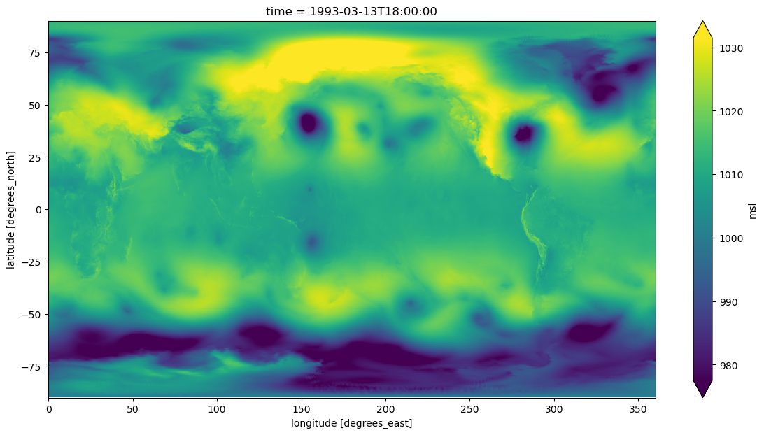
Plot the data on a map
nx,ny = np.meshgrid(longitude,latitude,indexing='ij')
timeStr = '1993-03-13T18:00'

tl1 = f'ERA-5 SLP (hPa)'
tl2 = f'Valid at: {timeStr}'
title_line = (tl1 + '\n' + tl2 + '\n') # concatenate the two strings and add return characters
cint = np.arange(900,1080,4)
res = '50m'
fig = plt.figure(figsize=(15,10))
ax = plt.subplot(1,1,1,projection=ccrs.PlateCarree())
#ax.set_extent ([lonW+constrainLon,lonE-constrainLon,latS+constrainLat,latN-constrainLat])
ax.add_feature(cfeature.COASTLINE.with_scale(res))
ax.add_feature(cfeature.STATES.with_scale(res))
#CL = slp.cf.plot.contour(levels=cint,linewidths=1.25,colors='green')
CL = ax.contour(nx, ny, slp, transform=ccrs.PlateCarree(),levels=cint, linewidths=1.25, colors='green')
ax.clabel(CL, inline_spacing=0.2, fontsize=11, fmt='%.0f')

title = plt.title(title_line,fontsize=16)
/home/runner/miniconda3/envs/ERA5_interactive/lib/python3.11/site-packages/cartopy/io/__init__.py:241: DownloadWarning: Downloading: https://naturalearth.s3.amazonaws.com/50m_physical/ne_50m_coastline.zip
  warnings.warn(f'Downloading: {url}', DownloadWarning)
/home/runner/miniconda3/envs/ERA5_interactive/lib/python3.11/site-packages/cartopy/io/__init__.py:241: DownloadWarning: Downloading: https://naturalearth.s3.amazonaws.com/50m_cultural/ne_50m_admin_1_states_provinces_lakes.zip
  warnings.warn(f'Downloading: {url}', DownloadWarning)
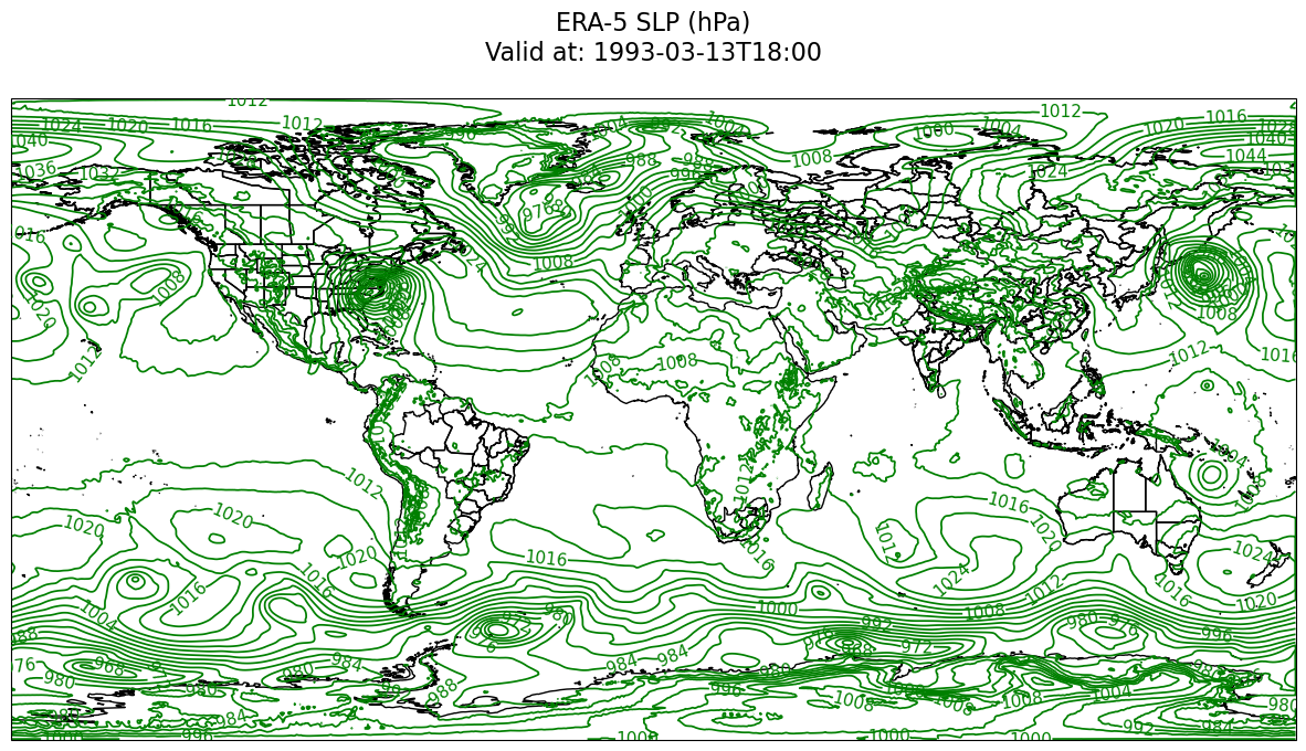
Summary
In this notebook, we have accessed one of the ARCO ERA-5 datasets, regridded from the ECMWF native spectral to cartesian lat-lon coordinates, and created a map of sea-level pressure for a particular date and time.
What’s next?
In the next notebook, we will leverage the Holoviz ecosystem and create interactive visualizations of the ARCO ERA-5 datasets.
Resources and references
This notebook follows the general workflow as used in the Google Research ARCO-ERA5 Surface Reanlysis Walkthrough notebook