Plotting HRRR 2-meter temperatures

Overview

Access archived HRRR data hosted on AWS in Zarr format
Visualize one of the variables (2m temperature) at an analysis time

Prerequisites

Concepts	Importance	Notes
Xarray Lessons 1-9	Necessary

Time to learn: 30 minutes

Imports

import xarray as xr
import s3fs
import metpy
import numpy as np
import matplotlib.pyplot as plt
import cartopy.crs as ccrs
import cartopy.feature as cfeature

What is Zarr?

So far we have used Xarray to work with gridded datasets in NetCDF and GRIB formats. Zarr is a relatively new data format. It is particularly relevant in the following two scenarios:

Datasets that are stored in what’s called object store. This is a commonly-used storage method for cloud providers, such as Amazon, Google, and Microsoft.
Datasets that are typically too large to load into memory all at once.

The Pangeo project specifically recommends Zarr as the Xarray-amenable data format of choice in the cloud:

“Our current preference for storing multidimensional array data in the cloud is the Zarr format. Zarr is a new storage format which, thanks to its simple yet well-designed specification, makes large datasets easily accessible to distributed computing. In Zarr datasets, the arrays are divided into chunks and compressed. These individual chunks can be stored as files on a filesystem or as objects in a cloud storage bucket. The metadata are stored in lightweight .json files. Zarr works well on both local filesystems and cloud-based object stores. Existing datasets can easily be converted to zarr via xarray’s zarr functions.”

Access archived HRRR data hosted on AWS in Zarr format

For a number of years, the Mesowest group at the University of Utah has hosted an archive of data from NCEP’s High Resolution Rapid Refresh model. This data, originally in GRIB-2 format, has been converted into Zarr and is freely available “in the cloud”, on Amazon Web Service’s Simple Storage Service, otherwise known as S3. Data is stored in S3 in a manner akin to (but different from) a Linux filesystem, using a bucket and object model.

To interactively browse the contents of this archive, go to this link: HRRRZarr File Browser on AWS

To access Zarr-formatted data stored in an S3 bucket, we follow a 3-step process:

Create URL(s) pointing to the bucket and object(s) that contain the data we want
Create map(s) to the object(s) with the s3fs library’s S3Map method
Pass the map(s) to Xarray’s open_dataset or open_mfdataset methods, and specify zarr as the format, via the engine argument.

A quirk in how these grids were converted from GRIB2 to Zarr means that the dimension variables are defined one directory up from where the data variables are. Thus, our strategy is to use Xarray's open_mfdataset method and pass in two AWS S3 file references to these two corresponding directories.

Create the URLs

date = '20211016'
hour = '21'
var = 'TMP'
level = '2m_above_ground'
url1 = 's3://hrrrzarr/sfc/' + date + '/' + date + '_' + hour + 'z_anl.zarr/' + level + '/' + var + '/' + level
url2 = 's3://hrrrzarr/sfc/' + date + '/' + date + '_' + hour + 'z_anl.zarr/' + level + '/' + var
print(url1)
print(url2)

s3://hrrrzarr/sfc/20211016/20211016_21z_anl.zarr/2m_above_ground/TMP/2m_above_ground
s3://hrrrzarr/sfc/20211016/20211016_21z_anl.zarr/2m_above_ground/TMP

In this case, hrrrzarr is the S3 bucket name. 2m_above_ground and TMP are both objects within the bucket. The former object has the 2-meter temperature array, while the latter contains the coordinate arrays of the spatial dimensions of 2m temperature (i.e., x and y).

Create the S3 maps from the S3 object store.

fs = s3fs.S3FileSystem(anon=True)
file1 = s3fs.S3Map(url1, s3=fs)
file2 = s3fs.S3Map(url2, s3=fs)

Use Xarray’s open_mfdataset to create a Dataset from these two S3 objects.

ds = xr.open_mfdataset([file1,file2], engine='zarr')

Examine the dataset.

ds

<xarray.Dataset> Size: 4MB
Dimensions:                  (projection_y_coordinate: 1059,
                              projection_x_coordinate: 1799)
Coordinates:
  * projection_x_coordinate  (projection_x_coordinate) float64 14kB -2.698e+0...
  * projection_y_coordinate  (projection_y_coordinate) float64 8kB -1.587e+06...
Data variables:
    TMP                      (projection_y_coordinate, projection_x_coordinate) float16 4MB dask.array<chunksize=(150, 150), meta=np.ndarray>
    forecast_period          timedelta64[ns] 8B ...
    forecast_reference_time  datetime64[ns] 8B ...
    height                   float64 8B ...
    pressure                 float64 8B ...
    time                     datetime64[ns] 8B ...

The projection information for the HRRR was not readily found in the Zarr representation, so we will need to define the relevant parameters explicitly from other sources, shown below.

HRRR Grid Navigation:

 PROJECTION:          LCC                 
 ANGLES:                38.5   -97.5    38.5
 GRID SIZE:             1799    1059
 LL CORNER:            21.1381 -122.7195
 UR CORNER:            47.8422  -60.9168

lon1 = -97.5
lat1 = 38.5
slat = 38.5
projData= ccrs.LambertConformal(central_longitude=lon1,
                             central_latitude=lat1,
                             standard_parallels=[slat,slat],globe=ccrs.Globe(semimajor_axis=6371229,
                                        semiminor_axis=6371229))

Note: The HRRR's projection assumes a spherical earth, whose semi-major/minor axes are both equal to 6371.229 km. We therefore need to explicitly define a Globe in Cartopy with these values.

Examine the dataset’s coordinate variables. Each x- and y- value represents distance in meters from the central latitude and longitude.

ds.coords

Coordinates:
  * projection_x_coordinate  (projection_x_coordinate) float64 14kB -2.698e+0...
  * projection_y_coordinate  (projection_y_coordinate) float64 8kB -1.587e+06...

Create an object pointing to the dataset’s data variable.

airTemp = ds.TMP

When we examine the object, we see that it is a special type of DataArray … a DaskArray.

airTemp

<xarray.DataArray 'TMP' (projection_y_coordinate: 1059,
                         projection_x_coordinate: 1799)> Size: 4MB
dask.array<open_dataset-TMP, shape=(1059, 1799), dtype=float16, chunksize=(150, 150), chunktype=numpy.ndarray>
Coordinates:
  * projection_x_coordinate  (projection_x_coordinate) float64 14kB -2.698e+0...
  * projection_y_coordinate  (projection_y_coordinate) float64 8kB -1.587e+06...
Attributes:
    GRIB_PARAM:  [2, 0, 0, 0]
    long_name:   2m_above_ground/TMP
    units:       K

Sidetrip: Dask

Dask is a Python library that is especially well-suited for handling very large datasets (especially those that are too large to fit into RAM) and is nicely integrated with Xarray. We're going to defer a detailed exploration of Dask for now. But suffice it to say that when we use open_mfdataset, the resulting objects are Dask objects.

MetPy supports Dask arrays, and so performing a unit conversion is straightforward.

airTemp = airTemp.metpy.convert_units('degC')

Verify that the object has the unit change

airTemp

<xarray.DataArray 'TMP' (projection_y_coordinate: 1059,
                         projection_x_coordinate: 1799)> Size: 4MB
<Quantity(dask.array<truediv, shape=(1059, 1799), dtype=float16, chunksize=(150, 150), chunktype=numpy.ndarray>, 'degree_Celsius')>
Coordinates:
  * projection_x_coordinate  (projection_x_coordinate) float64 14kB -2.698e+0...
  * projection_y_coordinate  (projection_y_coordinate) float64 8kB -1.587e+06...
Attributes:
    GRIB_PARAM:  [2, 0, 0, 0]
    long_name:   2m_above_ground/TMP

Similar to what we did for datasets whose projection-related coordinates were latitude and longitude, we define objects pointing to x and y now, so we can pass them to the plotting functions.

x = airTemp.projection_x_coordinate
y = airTemp.projection_y_coordinate

Visualize 2m temperature at an analysis time

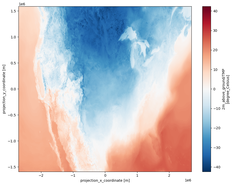
First, just use Xarray’s plot function to get a quick look to verify that things look right.

airTemp.plot(figsize=(11,8.5))

<matplotlib.collections.QuadMesh at 0x7f09154bc830>

../../_images/0fe99d791670a93a51556924c6bbed3742dc3681a6fb73c1229cc6b75f5c5fc5.png

To facilitate the bounds of the contour intervals, obtain the min and max values from this DataArray.

A Dask array is even more lazy in terms of its data loading than a basic DataArray in Xarray. If we want to perform a computation on this array, e.g. calculate the mean, min, or max, note that we don't get a result straightaway ... we get another Dask array.

airTemp.min()

<xarray.DataArray 'TMP' ()> Size: 2B
array(-4.75, dtype=float16)

With Dask arrays, applying the min and max functions doesn't actually do the computation ... instead, it is creating a task graph which describes how the computations would be launched. You will need to call Dask's compute function to actually trigger the computation.

minTemp = airTemp.min().compute()
maxTemp = airTemp.max().compute()

minTemp.values, maxTemp.values

(array(-4.75, dtype=float16), array(38.75, dtype=float16))

Based on the min and max, define a range of values used for contouring. Let’s invoke NumPy’s floor and ceil(ing) functions so these values conform to whatever variable we are contouring.

fint = np.arange(np.floor(minTemp.values),np.ceil(maxTemp.values) + 2, 2)

fint

array([-5., -3., -1.,  1.,  3.,  5.,  7.,  9., 11., 13., 15., 17., 19.,
       21., 23., 25., 27., 29., 31., 33., 35., 37., 39.])

For a single map, setting the contour fill values as we did above is appropriate. But if you were producing a series of maps that span a range of times, a consistent (and thus wider) range of values would be better.

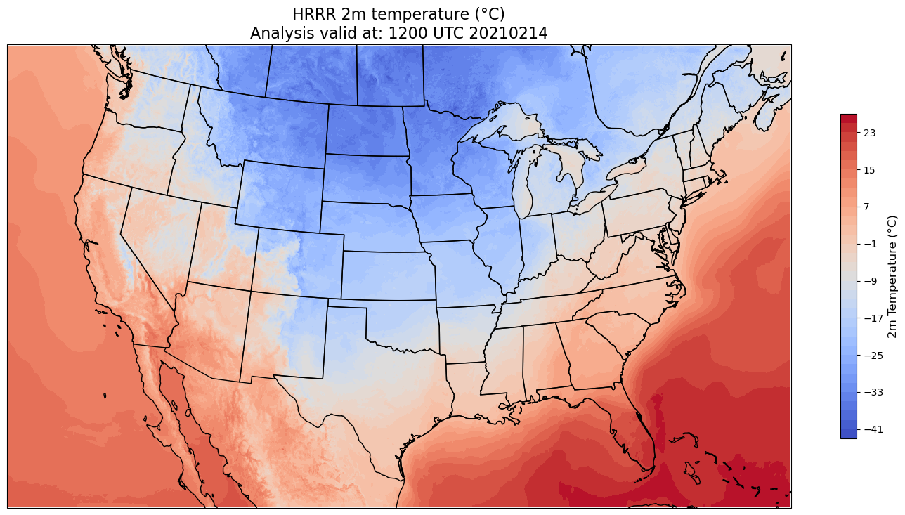
Plot the map

We’ll define the plot extent to nicely encompass the HRRR’s spatial domain.

latN = 50.4
latS = 24.25
lonW = -123.8
lonE = -71.2

res = '50m'

fig = plt.figure(figsize=(18,12))
ax = plt.subplot(1,1,1,projection=projData)
ax.set_extent ([lonW,lonE,latS,latN],crs=ccrs.PlateCarree())
ax.add_feature(cfeature.COASTLINE.with_scale(res))
ax.add_feature(cfeature.STATES.with_scale(res))

# Add the title
tl1 = str('HRRR 2m temperature ($^\circ$C)')
tl2 = str('Analysis valid at: '+ hour + '00 UTC ' + date  )
plt.title(tl1+'\n'+tl2,fontsize=16)

# Contour fill
CF = ax.contourf(x,y,airTemp,levels=fint,cmap=plt.get_cmap('coolwarm'))
# Make a colorbar for the ContourSet returned by the contourf call.
cbar = fig.colorbar(CF,shrink=0.5)
cbar.set_label(r'2m Temperature ($^\circ$C)', size='large')

../../_images/64bd7799c19af8d22b9aed64ce517a1f7dd332fa9eb8a4e548e826f9ebe16d4e.png

Summary

Xarray can access datasets in Zarr format, which is ideal for a cloud-based object store system such as S3.
Xarray and MetPy both support Dask, a library that is particularly well-suited for very large datasets.

What’s next?

On your own, browse the hrrrzarr S3 bucket. Try making maps for different variables and/or different times.