Atmospheric Sciences Research Center Whiteface Mountain Field Station logo

Whiteface Mountain Cloud Water Data¶

Accessing Cloud Water Data from the ASRC¶

Overview¶

Cloud water data provide an insight into the chemical processing of gasses and particulates in the atmosphere. While this is not technically an API, this notebook will show how to access a niche dataset for cloud water chemistry, collected in-situ at Whiteface Mountain in Wilmington, NY. The sample site serves as a relative background for atmospheric chemistry within the region, as it is a remote, mountain-top observatory.

This notebook will cover

Requesting data access
Cleaning and sorting through the data
Basic cloud water chemistry analysis (Coming Soon)
Plotting the data (Coming Soon)

Prerequisites¶

Concepts	Importance	Notes
Introduction to Pandas	Necessary	How to deal with dataframes and datasets
Matplotlib Basics	Helpful	Skills for different plotting styles and techniques

Time to learn: 45 minutes
System requirements:
- Email Address for Data Access

Imports¶

Info

Here we'll import lots of stuff, but we might not end up using them all...

import matplotlib.pyplot as plt
import seaborn as sns
import pandas as pd
from datetime import date
from datetime import datetime
import numpy as np

We will also set some limits to the size of data that Pandas displays, so as not to overload our screens.

# Set the maximum number of rows and columns to display
pd.set_option('display.max_rows', 10)  # Set to the number of rows you want to display
pd.set_option('display.max_columns', 10)  # Set to the number of columns you want to display

Accessing the Data¶

Currently, the data from the Whiteface Mountain summit are obtained and managed by the Lance Research Laboratory. Available data includes, among others, chemical speciation within cloud water:

Anions	Cations
Sulfate	Ammonium
Nitrate	Sodium
Chloride	Calcium
Formate	Magnesium
Acetate	Potassium
Oxalate

Some Other Data
Total Organic Carbon
pH
Conductivity
Liquid Water Content
Sample Volume
Sample Dump Date/Time

Note:

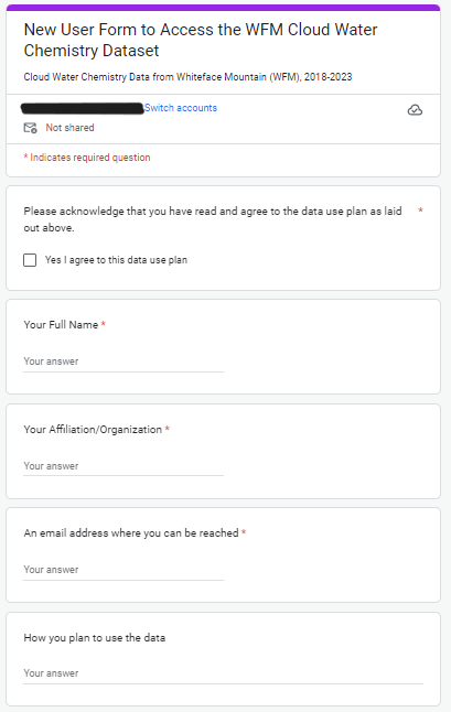
In order to access the data, we don't need an API. We just need to fill out a simple `Google Form` at the following website:

http://atmoschem.asrc.cestm.albany.edu/~cloudwater/pub/Data.htm

WFM Data Form

Once you are granted access, you can utilize recent and historical data spanning back to 1994.
The data come in *.xlsx files, or as multiple *.xlsx files in a zip drive, depending on which dataset you collect.

This notebook uses 2022 Cloud Water Data (current as of June 18th, 2024) as an example.
As the data files come with various sheets covering multiple angles of quality control, we will simplify this notebook with a *.csv file of the “valid” samples.

The full data file can be viewed in ../files/WFC.2022.Data.R2--6_18_24.xlsx.

Reading the Data¶

We will utilize the Pandas package to handle our reading in our data file. We will also preemptively use the ISO-8859-1 encoding to ensure symbols like ° and μ work.

df = pd.read_csv('../files/WFC.2022.Data.R2--6_18_24.csv', encoding = 'ISO-8859-1')

Let’s look at our dataframe...

df

As we can see above, the data actually begin on the fifth line.

Let’s take a closer look and notice that there are only 42 samples in this particular set...

df.iloc[4:50,:]

In the next cell, we will use Row 4 for our column headings, and slice the dataframe so it only shows our data. Cleaning up the data is helpful for preemptively halting any errors resulting from NaNs and empty cells.

df.columns = df.iloc[4]
df = df.iloc [5:48]
df

Some brief details about the data format...

The LABNO values represent the Julian date, where the first two digits are year, and the next three are the day. The remaining two digits refer to internal identification regarding the collection bottles for same-day samples.

The cloud water at Whiteface Mountain is collected in bulk 12-hour samples, so the time the accumulated sample was "dumped" into a storage container is in the DUMP TIME column, and the duration of time in that 12-hour period where the summit was in-cloud is show in in the COLLECTION_HOURS column.

Let’s look at all the columns that have data in them below...

for col in df.columns:
    if not df[col].isna().all():
        print(col)

LABNO
DUMP TIME
COLLECTION_HOURS
POOL_VOL ml
LWC g m-3
TEMP °C
WINDDIR_AVG °AZ
OCTANT
AVG_S_WSP m s-1
LABPH
SPCOND µS cm-1
HION µeq L-1
CA mg L-1
CA µeq L-1
MG mg L-1
MG µeq L-1
NA mg L-1
NA µeq L-1
K mg L-1
K µeq L-1
NH4 mg L-1
NH4 µeq L-1
SO4 mg L-1
SO4 µeq L-1
NO3 mg L-1
NO3 µeq L-1
CL mg L-1
CL µeq L-1
TOC µmols C L-1
TN_F
COMMENT
CATION_ANION_RATIO
SUM_CATIONS µeq L-1
SUM_ANIONS µeq L-1
RPD
Glyoxalate_ppb
Formate_ppb
AcetateGlycolate_ppb
Lactate_ppb
Malonate_ppb
Oxalate_ppb
Pyruvate_ppb
SuccinateMalate_ppb

Now that we have our data in a manageable format, we can begin any analysis or visualizations we are interested in.

Analyzing the Data¶

Coming Soon!

This section is still under development.

Plotting the Data¶

Coming Soon!

This section is still under development.

Summary¶

In this notebook, we’ve covered how to access cloud water chemistry data from the Lance Research Laboratory at the University at Albany’s Atmospheric Sciences Research Center. We’ve looked at the data format, and ways to process and analyze the data. This is a niche dataset, updated regularly as cloud water is collected, processed, and analyzed each summer.

Resources and references¶

More information about the Whiteface Mountain Field Station: https://whiteface.asrc.albany.edu/

More information about the Lance Research Laboratory: https://research.asrc.albany.edu/facstaff/lance/index.html

More information about the cloud water chemistry at Whiteface Mountain: https://acp.copernicus.org/articles/23/1619/2023/

Information about the author: Adam Deitsch

Example Workflows

Data access via earthaccess library and vizualization with cartopy