Cloud Condensation Nuclei and Precipitation Analysis
Example shows how to plot up CCN droplet count in a size distribution plot, and an interactive precipitation intensity visualization.
Imports
import numpy as np
import act
import matplotlib.pyplot as plt
import plotly.graph_objects as go
Analyze CCN Data for BNF from the Data Archive
username = 'mgrover4'
token = '176e1559b67be630'
datastream = 'bnfaosccn2colaspectraM1.b1'
startdate = '2025-05-08'
enddate = '2025-05-11T23:59:59'
# Download and read the data
result_ccn = act.discovery.download_arm_data(username, token, datastream, startdate, enddate)
ds_ccn = act.io.read_arm_netcdf(result_ccn)
ds_ccn.clean.cleanup()[DOWNLOADING] bnfaosccn2colaspectraM1.b1.20250508.010251.nc
[DOWNLOADING] bnfaosccn2colaspectraM1.b1.20250509.000954.nc
[DOWNLOADING] bnfaosccn2colaspectraM1.b1.20250510.002958.nc
[DOWNLOADING] bnfaosccn2colaspectraM1.b1.20250511.005002.nc
If you use these data to prepare a publication, please cite:

Koontz, A., Uin, J., Andrews, E., Enekwizu, O., Hayes, C., & Salwen, C. Cloud
Condensation Nuclei Particle Counter (AOSCCN2COLASPECTRA), 2025-05-08 to
2025-05-11, Bankhead National Forest, AL, USA; Long-term Mobile Facility (BNF),
Bankhead National Forest, AL, AMF3 (Main Site) (M1). Atmospheric Radiation
Measurement (ARM) User Facility. https://doi.org/10.5439/1323896
/home/runner/micromamba/envs/arm-field-site-cookbook-dev/lib/python3.11/site-packages/act/io/arm.py:155: FutureWarning: In a future version of xarray the default value for data_vars will change from data_vars='all' to data_vars=None. This is likely to lead to different results when multiple datasets have matching variables with overlapping values. To opt in to new defaults and get rid of these warnings now use `set_options(use_new_combine_kwarg_defaults=True) or set data_vars explicitly.
  ds = xr.open_mfdataset(filenames, **kwargs)
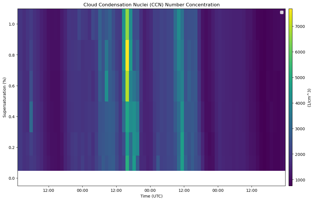
Visualize the CCN Data
if 'lat' not in ds_ccn.coords:
    ds_ccn = ds_ccn.set_coords(['lat', 'lon'])

print("Variables:", list(ds_ccn.data_vars))

ccn_var = 'concentration'

# Plot
disp = act.plotting.TimeSeriesDisplay(ds_ccn, figsize=(12, 8))
disp.plot(ccn_var, label='CCN Concentration [#/cm³]')
disp.axes[0].set_title('Cloud Condensation Nuclei (CCN) Number Concentration')
disp.axes[0].set_ylabel('Supersaturation (%)')
disp.axes[0].set_xlabel('Time (UTC)')
disp.day_night_background()
disp.axes[0].legend()

plt.show()
Variables: ['base_time', 'time_offset', 'time_bounds', 'setpoint_time', 'supersaturation_calculated', 'N_CCN', 'qc_N_CCN', 'N_CCN_fit_coefs', 'N_CCN_fit_error', 'N_CCN_fit_value', 'concentration', 'f_CCN', 'qc_f_CCN', 'alt']
/tmp/ipykernel_3989/132956031.py:15: UserWarning: Legend does not support handles for QuadMesh instances.
See: https://matplotlib.org/stable/tutorials/intermediate/legend_guide.html#implementing-a-custom-legend-handler
  disp.axes[0].legend()
/tmp/ipykernel_3989/132956031.py:15: UserWarning: No artists with labels found to put in legend.  Note that artists whose label start with an underscore are ignored when legend() is called with no argument.
  disp.axes[0].legend()
#Get supersaturation levels and time
supersat = ds_ccn['supersaturation_setpoint'].values
times = ds_ccn['time'].values

#Create the plot
fig, ax = plt.subplots(figsize=(12, 5))
colors = plt.cm.viridis(np.linspace(0, 1, len(supersat)))

#Plot one trace per supersaturation level
for i, ss in enumerate(supersat):
    ccn = ds_ccn['concentration'].sel(supersaturation_setpoint=ss)
    valid = ~ccn.isnull()
    ax.scatter(times[valid], ccn.values[valid], s=10, color=colors[i], label=f'SS = {ss:.2f}')

#Plot makeup
ax.set_title('CCN Number Concentration vs Time at Different Supersaturations')
ax.set_xlabel('Time (UTC)')
ax.set_ylabel('CCN Concentration [#/cm³]')
ax.set_yscale('log')
ax.legend(title='Supersaturation (%)')
ax.grid(True)
plt.tight_layout()
plt.show()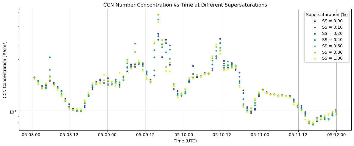
Precipitation Analysis with the Pluvio
# Set the datastream and start/enddates
datastream = 'bnfwbpluvio2M1.a1'
startdate = '2025-05-08'
enddate = '2025-05-11T23:59:59'
# Use ACT to easily download the data. Watch for the data citation! Show some support
# for ARM's instrument experts and cite their data if you use it in a publication
result_rain = act.discovery.download_arm_data(username, token, datastream, startdate, enddate)
# Let's read in the data using ACT and check out the data
ds_rain = act.io.read_arm_netcdf(result_rain)
# Apply quality control checks
ds_rain.clean.cleanup()[DOWNLOADING] bnfwbpluvio2M1.a1.20250508.000000.nc
[DOWNLOADING] bnfwbpluvio2M1.a1.20250509.000000.nc
[DOWNLOADING] bnfwbpluvio2M1.a1.20250510.000000.nc
[DOWNLOADING] bnfwbpluvio2M1.a1.20250511.000000.nc
If you use these data to prepare a publication, please cite:

Zhu, Z., Wang, D., Jane, M., Cromwell, E., Sturm, M., Irving, K., & Delamere, J.
Weighing Bucket Precipitation Gauge (WBPLUVIO2), 2025-05-08 to 2025-05-11,
Bankhead National Forest, AL, USA; Long-term Mobile Facility (BNF), Bankhead
National Forest, AL, AMF3 (Main Site) (M1). Atmospheric Radiation Measurement
(ARM) User Facility. https://doi.org/10.5439/1338194
/home/runner/micromamba/envs/arm-field-site-cookbook-dev/lib/python3.11/site-packages/act/io/arm.py:155: FutureWarning: In a future version of xarray the default value for data_vars will change from data_vars='all' to data_vars=None. This is likely to lead to different results when multiple datasets have matching variables with overlapping values. To opt in to new defaults and get rid of these warnings now use `set_options(use_new_combine_kwarg_defaults=True) or set data_vars explicitly.
  ds = xr.open_mfdataset(filenames, **kwargs)
#printing output label
print("Available rain-related variables:")
#printing list of variables
print(list(ds_rain.data_vars))
#saving rain variables
rain_rate_var = 'intensity_rt'
#giving a shortcut
ds = ds_rain
Available rain-related variables:
['base_time', 'time_offset', 'intensity_rt', 'accum_rtnrt', 'accum_nrt', 'accum_total_nrt', 'bucket_rt', 'bucket_nrt', 'load_cell_temp', 'heater_status', 'pluvio_status', 'elec_unit_temp', 'supply_volts', 'orifice_temp', 'maintenance_flag', 'reset_flag', 'volt_min', 'ptemp', 'intensity_rtnrt', 'lat', 'lon', 'alt']
Interactive Visualizion of the Pluvio Data
#store data
rain_rate_var = 'intensity_rt'
df_rain = ds_rain[rain_rate_var].to_dataframe().dropna()

fig = go.Figure()

fig.add_trace(go.Scatter(
    x=df_rain.index,
    y=df_rain[rain_rate_var],
    mode='lines+markers',
    name='Rain Rate [mm/hr]',
    line=dict(color='blue')
))

fig.update_layout(
    title='Rain Rate (Pluvio2)',
    xaxis_title='Time (UTC)',
    yaxis_title='Rain Rate [mm/hr]',
    hovermode='x unified',
    template='plotly_white',
    height=500,
)

fig.show()
Loading...