Aerosol Optical Properties at BNF
Imports
import act
import numpy as np
import pandas as pd
import xarray as xr
import matplotlib.pyplot as plt
import matplotlib.colors as colors
Access Aerosol Property Data at BNF
Use the ACT library to search and download data at BNF
# Set your username and token
username = 'mgrover4'
token = '176e1559b67be630'

# Set the datastream and start/enddates
datastream = 'bnfaoscaps3wM1.b1'
startdate = '2025-05-08'
enddate = '2025-05-11T23:59:59'

# Use ACT to easily download the data.  Watch for the data citation!  Show some support
# for ARM's instrument experts and cite their data if you use it in a publication
result_caps = act.discovery.download_arm_data(username, token, datastream, startdate, enddate)

datastream = 'bnfaossmpsM1.b1'
result_smps = act.discovery.download_arm_data(username, token, datastream, startdate, enddate)

datastream = 'bnfaosnephdryM1.b1'
result_neph = act.discovery.download_arm_data(username, token, datastream, startdate, enddate)

# Set the datastream and start/enddates
datastream = 'bnfmetM1.b1'
result_met = act.discovery.download_arm_data(username, token, datastream, startdate, enddate)

datastream = 'bnfaoppsap1flynn1mM1.c1'
result_psap = act.discovery.download_arm_data(username, token, datastream, startdate, enddate)

datastream = 'bnfaossp2xrM1.b1'
result_sp2 = act.discovery.download_arm_data(username, token, datastream, startdate, enddate)
[DOWNLOADING] bnfaoscaps3wM1.b1.20250508.000000.nc
[DOWNLOADING] bnfaoscaps3wM1.b1.20250509.000000.nc
[DOWNLOADING] bnfaoscaps3wM1.b1.20250510.000000.nc
[DOWNLOADING] bnfaoscaps3wM1.b1.20250511.000000.nc
If you use these data to prepare a publication, please cite:

Koontz, A., Sedlacek, A., & Smith, S. Cavity Attenuated Phase Shift Extinction
Monitor (AOSCAPS3W), 2025-05-08 to 2025-05-11, Bankhead National Forest, AL,
USA; Long-term Mobile Facility (BNF), Bankhead National Forest, AL, AMF3 (Main
Site) (M1). Atmospheric Radiation Measurement (ARM) User Facility.
https://doi.org/10.5439/1406888
[DOWNLOADING] bnfaossmpsM1.b1.20250508.000459.nc
[DOWNLOADING] bnfaossmpsM1.b1.20250509.000459.nc
[DOWNLOADING] bnfaossmpsM1.b1.20250510.000459.nc
[DOWNLOADING] bnfaossmpsM1.b1.20250511.000459.nc
If you use these data to prepare a publication, please cite:

Kuang, C., Singh, A., Howie, J., Salwen, C., & Hayes, C. Scanning mobility
particle sizer (AOSSMPS), 2025-05-08 to 2025-05-11, Bankhead National Forest,
AL, USA; Long-term Mobile Facility (BNF), Bankhead National Forest, AL, AMF3
(Main Site) (M1). Atmospheric Radiation Measurement (ARM) User Facility.
https://doi.org/10.5439/1476898
[DOWNLOADING] bnfaosnephdryM1.b1.20250508.000003.nc
[DOWNLOADING] bnfaosnephdryM1.b1.20250509.000001.nc
[DOWNLOADING] bnfaosnephdryM1.b1.20250510.000002.nc
[DOWNLOADING] bnfaosnephdryM1.b1.20250511.000003.nc
If you use these data to prepare a publication, please cite:

Koontz, A., Flynn, C., Uin, J., Jefferson, A., Andrews, E., Salwen, C., & Hayes,
C. Nephelometer (AOSNEPHDRY), 2025-05-08 to 2025-05-11, Bankhead National
Forest, AL, USA; Long-term Mobile Facility (BNF), Bankhead National Forest, AL,
AMF3 (Main Site) (M1). Atmospheric Radiation Measurement (ARM) User Facility.
https://doi.org/10.5439/1228051
[DOWNLOADING] bnfmetM1.b1.20250508.000000.cdf
[DOWNLOADING] bnfmetM1.b1.20250509.000000.cdf
[DOWNLOADING] bnfmetM1.b1.20250510.000000.cdf
[DOWNLOADING] bnfmetM1.b1.20250511.000000.cdf

If you use these data to prepare a publication, please cite:

Kyrouac, J., Shi, Y., & Tuftedal, M. Surface Meteorological Instrumentation
(MET), 2025-05-08 to 2025-05-11, Bankhead National Forest, AL, USA; Long-term
Mobile Facility (BNF), Bankhead National Forest, AL, AMF3 (Main Site) (M1).
Atmospheric Radiation Measurement (ARM) User Facility.
https://doi.org/10.5439/1786358
[DOWNLOADING] bnfaoppsap1flynn1mM1.c1.20250508.000030.nc
[DOWNLOADING] bnfaoppsap1flynn1mM1.c1.20250509.000030.nc
[DOWNLOADING] bnfaoppsap1flynn1mM1.c1.20250510.000030.nc
[DOWNLOADING] bnfaoppsap1flynn1mM1.c1.20250511.000030.nc

If you use these data to prepare a publication, please cite:

Koontz, A., Flynn, C., Shilling, J., & Flynn, C. Aerosol Optical Properties
(AOPPSAP1FLYNN1M), 2025-05-08 to 2025-05-11, Bankhead National Forest, AL, USA;
Long-term Mobile Facility (BNF), Bankhead National Forest, AL, AMF3 (Main Site)
(M1). Atmospheric Radiation Measurement (ARM) User Facility.
https://doi.org/10.5439/1369240
[DOWNLOADING] bnfaossp2xrM1.b1.20250508.000000.nc
[DOWNLOADING] bnfaossp2xrM1.b1.20250509.000000.nc
[DOWNLOADING] bnfaossp2xrM1.b1.20250510.000000.nc
[DOWNLOADING] bnfaossp2xrM1.b1.20250511.000001.nc
[DOWNLOADING] bnfaossp2xrM1.b1.20250511.204049.nc

If you use these data to prepare a publication, please cite:

Sedlacek, A., & Ermold, B. Single Particle Soot Photometer (AOSSP2XR),
2025-05-08 to 2025-05-11, Bankhead National Forest, AL, USA; Long-term Mobile
Facility (BNF), Bankhead National Forest, AL, AMF3 (Main Site) (M1). Atmospheric
Radiation Measurement (ARM) User Facility. https://doi.org/10.5439/2507427
Load the Data into ACT and Apply Quality Control
Let’s read in the data using ACT and check out the data
ds_caps_org = act.io.read_arm_netcdf(result_caps)
ds_smps_org = act.io.read_arm_netcdf(result_smps)
ds_neph_org = act.io.read_arm_netcdf(result_neph)
ds_sp2_org = act.io.read_arm_netcdf(result_sp2)
ds_psap_org = act.io.read_arm_netcdf(result_psap)
/home/runner/micromamba/envs/arm-field-site-cookbook-dev/lib/python3.11/site-packages/act/io/arm.py:155: FutureWarning: In a future version of xarray the default value for data_vars will change from data_vars='all' to data_vars=None. This is likely to lead to different results when multiple datasets have matching variables with overlapping values. To opt in to new defaults and get rid of these warnings now use `set_options(use_new_combine_kwarg_defaults=True) or set data_vars explicitly.
ds = xr.open_mfdataset(filenames, **kwargs)
/home/runner/micromamba/envs/arm-field-site-cookbook-dev/lib/python3.11/site-packages/act/io/arm.py:155: FutureWarning: In a future version of xarray the default value for data_vars will change from data_vars='all' to data_vars=None. This is likely to lead to different results when multiple datasets have matching variables with overlapping values. To opt in to new defaults and get rid of these warnings now use `set_options(use_new_combine_kwarg_defaults=True) or set data_vars explicitly.
  ds = xr.open_mfdataset(filenames, **kwargs)
Visualize the Data without Quality Control
display = act.plotting.TimeSeriesDisplay({'CAPS': ds_caps_org, 'NEPH':ds_neph_org,'SMPS': ds_smps_org }, figsize=(15, 10), subplot_shape=(3,))


# Plot up the variable in the first plot
# Need to specify the dsname so it knows which dataset
# to use for this data.  This is helpful when datasets
# have similar variable names
display.plot('Bext_R', dsname='CAPS', subplot_index=(0,),color='red',marker='o', linestyle='none',alpha=0.3)
display.plot('Bext_G', dsname='CAPS', subplot_index=(0,),color='green',marker='o', linestyle='none',alpha=0.3)
display.plot('Bext_B', dsname='CAPS', subplot_index=(0,),color='blue',marker='o', linestyle='none',alpha=0.3)


display.plot('Bs_R_Dry_Neph3W', dsname='NEPH', subplot_index=(1,),color='red',marker='o', linestyle='none',alpha=0.3)
display.plot('Bs_G_Dry_Neph3W', dsname='NEPH', subplot_index=(1,),color='green',marker='o', linestyle='none',alpha=0.3)
display.plot('Bs_B_Dry_Neph3W', dsname='NEPH', subplot_index=(1,),color='blue',marker='o', linestyle='none',alpha=0.3)

# Plot up the MET btemperature and precipitation
display.plot('dN_dlogDp', dsname='SMPS', subplot_index=(2,))
display.axes[2,].set_ylim(0, 300)
(0.0, 300.0)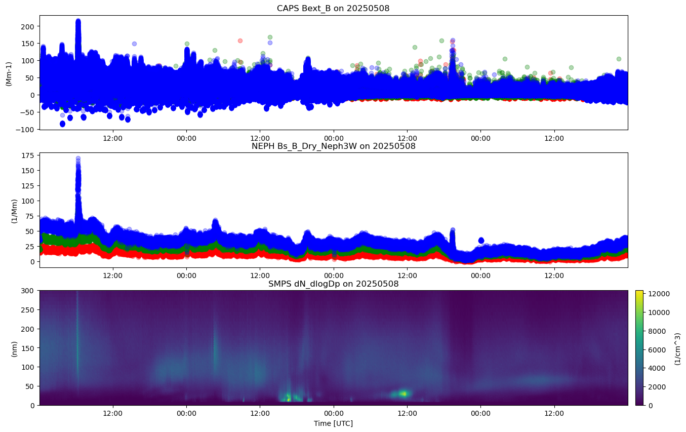
We can see that there’s some missing data in the plot above so let’s take a look at the embedded QC!
First, for many of the ACT QC features, we need to get the dataset more to CF standard and that involves cleaning up some of the attributes and ways that ARM has historically handled QC
ds_caps_org.clean.cleanup()
ds_smps_org.clean.cleanup()
ds_neph_org.clean.cleanup()
ds_sp2_org.clean.cleanup()
ds_psap_org.clean.cleanup()

ds_caps_org = ds_caps_org.load().where(ds_caps_org.impactor_state == 1, drop=True)
ds_neph_org = ds_neph_org.load().where(ds_neph_org.impactor_state == 1, drop=True)
ds_psap_org = ds_psap_org.load().where(ds_psap_org.impactor_state == 1, drop=True)

ds_psap_org
Loading...
Resample to Equivalent Hourly Frequency
And plot again!
Create a plotting display object with 2 plots.
Note we have to create a dictionary of datasets to pass in.
ds_caps=ds_caps_org.resample(time='60min').mean()
ds_neph=ds_neph_org.resample(time='60min').mean()
ds_psap=ds_psap_org.resample(time='60min').mean()
ds_sp2=ds_sp2_org.resample(time='60min').mean()
ds_smps=ds_smps_org.resample(time="60min").mean()
display = act.plotting.TimeSeriesDisplay({'CAPS': ds_caps, 'NEPH':ds_neph,'SMPS': ds_smps }, figsize=(15, 10), subplot_shape=(3,))
# Plot up the variable in the first plot
# Need to specify the dsname so it knows which dataset
# to use for this data. This is helpful when datasets
# have similar variable names
display.plot('Bext_R', dsname='CAPS', subplot_index=(0,),color='red',marker='o', linestyle='none',alpha=0.3)
display.plot('Bext_G', dsname='CAPS', subplot_index=(0,),color='green',marker='o', linestyle='none',alpha=0.3)
display.plot('Bext_B', dsname='CAPS', subplot_index=(0,),color='blue',marker='o', linestyle='none',alpha=0.3)
display.plot('Bs_R_Dry_Neph3W', dsname='NEPH', subplot_index=(1,),color='red',marker='o', linestyle='none',alpha=0.3)
display.plot('Bs_G_Dry_Neph3W', dsname='NEPH', subplot_index=(1,),color='green',marker='o', linestyle='none',alpha=0.3)
display.plot('Bs_B_Dry_Neph3W', dsname='NEPH', subplot_index=(1,),color='blue',marker='o', linestyle='none',alpha=0.3)
# Plot up the MET btemperature and precipitation
display.plot('dN_dlogDp', dsname='SMPS', subplot_index=(2,))
display.axes[2,].set_ylim(0, 300)(0.0, 300.0)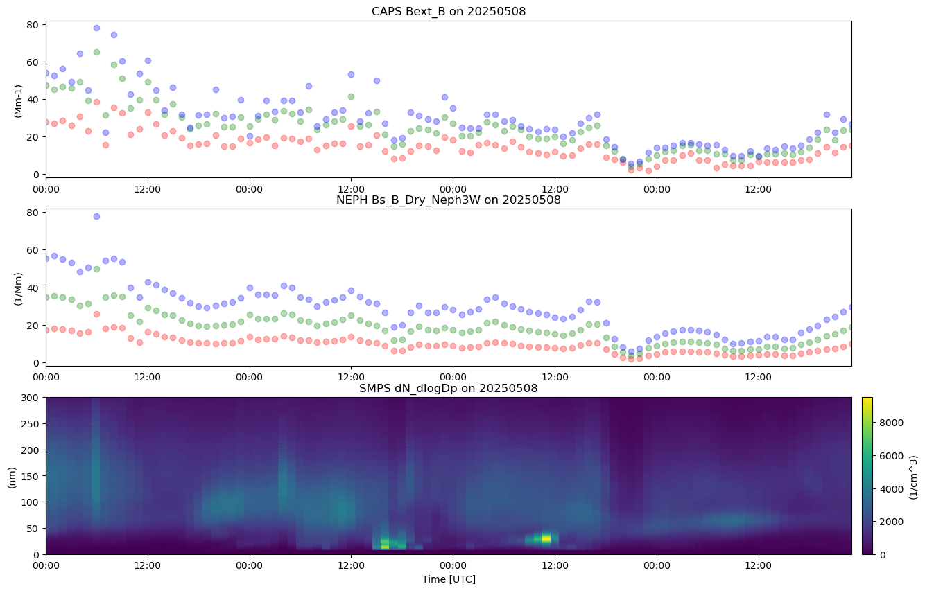
Create a Scatter Plot Comparison of Values
dfNeph=ds_neph.to_dataframe()
dfCaps=ds_caps.to_dataframe()
dfPsap=ds_psap.to_dataframe()
dfSp2=ds_sp2.to_dataframe()
df_merged = pd.merge_asof(dfCaps, dfPsap,on='time', direction='nearest')
df_merged['SSA B']=df_merged['Bs_B_Dry_Neph3W']/df_merged['Bext_B']
df_merged['SSA R']=df_merged['Bs_R_Dry_Neph3W']/df_merged['Bext_R']
df_merged['SSA G']=df_merged['Bs_G_Dry_Neph3W']/df_merged['Bext_G']
df_merged['alphaRB']=-(np.log (df_merged['Bs_R_Dry_Neph3W']/df_merged['Bs_B_Dry_Neph3W'])/np.log (700/450))
df_merged['alphaBG']=-(np.log (df_merged['Bs_B_Dry_Neph3W']/df_merged['Bs_G_Dry_Neph3W'])/np.log (450/550))
df_merged['alphaGR']=-(np.log (df_merged['Bs_G_Dry_Neph3W']/df_merged['Bs_R_Dry_Neph3W'])/np.log (550/700))
df_merged['Abs_B']=df_merged['Bext_B']-df_merged['Bs_B_Dry_Neph3W']
df_merged['Abs_R']=df_merged['Bext_R']-df_merged['Bs_R_Dry_Neph3W']
df_merged['Abs_G']=df_merged['Bext_G']-df_merged['Bs_G_Dry_Neph3W']
df_merged['AAE_RB']=-(np.log (df_merged['Abs_R']/df_merged['Abs_B'])/np.log (700/450))
df_merged['AAE_BG']=-(np.log (df_merged['Abs_B']/df_merged['Abs_G'])/np.log (450/550))
df_merged['AAE_GR']=-(np.log (df_merged['Abs_G']/df_merged['Abs_R'])/np.log (550/700))
df_merged['Avg_SAE']=(df_merged['alphaRB']+df_merged['alphaBG']+df_merged['alphaGR'])/3
df_merged['Avg_SSA']=(df_merged['SSA B']+df_merged['SSA R']+df_merged['SSA G'])/3/home/runner/micromamba/envs/arm-field-site-cookbook-dev/lib/python3.11/site-packages/pandas/core/arraylike.py:399: RuntimeWarning: invalid value encountered in log
result = getattr(ufunc, method)(*inputs, **kwargs)
/home/runner/micromamba/envs/arm-field-site-cookbook-dev/lib/python3.11/site-packages/pandas/core/arraylike.py:399: RuntimeWarning: invalid value encountered in log
result = getattr(ufunc, method)(*inputs, **kwargs)
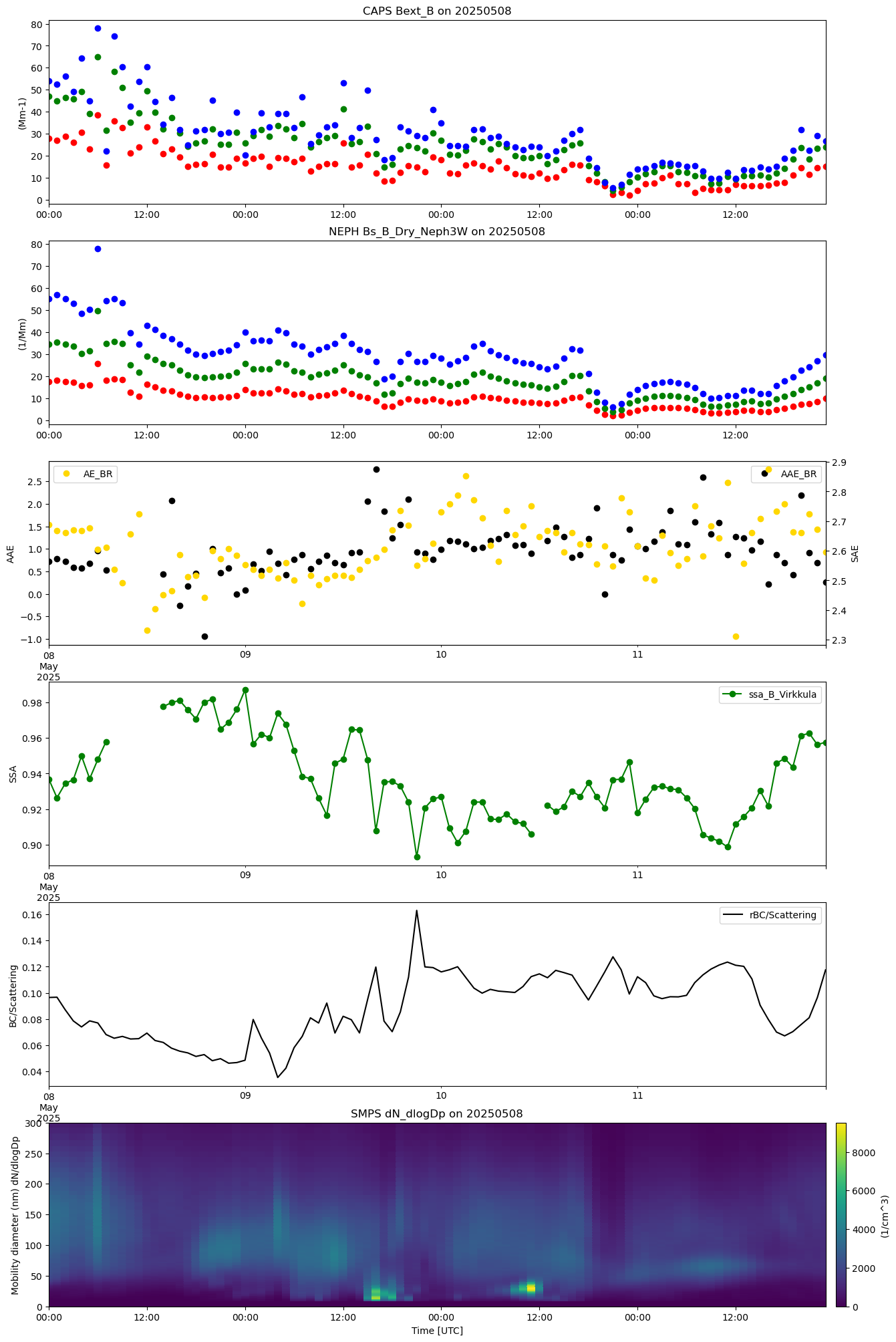
display = act.plotting.TimeSeriesDisplay({'CAPS': ds_caps, 'NEPH':ds_neph,'SMPS': ds_smps }, figsize=(15, 25), subplot_shape=(6,))


# Plot up the variable in the first plot
# Need to specify the dsname so it knows which dataset
# to use for this data.  This is helpful when datasets
# have similar variable names
display.plot('Bext_R', dsname='CAPS', subplot_index=(0,),color='red',marker='o', linestyle='none',alpha=1)
display.plot('Bext_G', dsname='CAPS', subplot_index=(0,),color='green',marker='o', linestyle='none',alpha=1)
display.plot('Bext_B', dsname='CAPS', subplot_index=(0,),color='blue',marker='o', linestyle='none',alpha=1)

display.plot('Bs_R_Dry_Neph3W', dsname='NEPH', subplot_index=(1,),color='red',marker='o', linestyle='none',alpha=1)
display.plot('Bs_G_Dry_Neph3W', dsname='NEPH', subplot_index=(1,),color='green',marker='o', linestyle='none',alpha=1)
display.plot('Bs_B_Dry_Neph3W', dsname='NEPH', subplot_index=(1,),color='blue',marker='o', linestyle='none',alpha=1)

#display.axes[2,].plot(df_merged['time'],df_merged['SSA R'], color='red',marker='o', linestyle='none',alpha=0.3)
#display.axes[2,].plot(df_merged['time'],df_merged['SSA G'],color='green',marker='o', linestyle='none',alpha=0.3)
#display.axes[2,].plot(df_merged['time'],df_merged['SSA B'],color='blue',marker='o', linestyle='none',alpha=0.3)

#df_merged.plot(x='time',y='SSA R',ax=display.axes[2,],color='red',style='o')
##df_merged.plot(x='time',y='SSA B',ax=display.axes[2,],color='blue',style='o')
#df_merged.plot(x='time',y='SSA G',ax=display.axes[2,],color='green',style='o')


#display.axes[2,].set_ylabel('SSA')
#display.axes[2,].set_ylim(0.25, 1.5)


df_merged.plot(x='time',y='AAE_BR',ax=display.axes[2,],color='black',style='o')


display.axes[2,].set_ylabel('AAE')
twinx=display.axes[2,].twinx()
twinx.set_ylabel('SAE')
df_merged.plot(x='time',y='AE_BR',ax=twinx,color='gold',style='o')
#twinx.set_ylim(1.5, 3)


#df_merged.plot(x='time',y='AAE_RB',ax=display.axes[4,],color='red',style='o')
##df_merged.plot(x='time',y='AAE_BG',ax=display.axes[4,],color='blue',style='o')
#df_merged.plot(x='time',y='AAE_GR',ax=display.axes[4,],color='green',style='o')
#display.axes[4,].set_ylabel('AAE')
#display.axes[4,].set_ylim(0, 2)

df_merged.plot(x='time',y='ssa_B_Virkkula',ax=display.axes[3,],color='green',style='-o')
display.axes[3,].set_ylabel('SSA')

#display.axes[3,].set_ylim(0.6, 1)
#twin_ax.set_ylim(0, 1)
dfSp2 = pd.DataFrame({'time': ds_sp2['time'].values, 'rBC_particle_conc': ds_sp2['rBC_particle_conc'].values, 'scattering_particle_conc': ds_sp2['scattering_particle_conc'].values})
dfSp2['rBC/Scattering']=dfSp2['rBC_particle_conc']/dfSp2['scattering_particle_conc']


dfSp2.plot(x='time',y='rBC/Scattering', color='black', ax=display.axes[4,])
display.axes[4,].set_ylabel('BC/Scattering')


display.plot('dN_dlogDp', dsname='SMPS', subplot_index=(5,))
display.axes[5,].set_ylim(0, 300)
display.axes[5,].set_ylabel('Mobility diameter (nm) dN/dlogDp')