Source determination through NOAA HYSPLIT trajectory model


HYSPLIT models simulate the dispersion and trajectory of substances transported and dispersed through our atmosphere, over local to global scales.
A common application is a back trajectory analysis to determine the origin of air masses and establish source-receptor relationships.
# import libraries
import xarray as xr   # for data storage and processing
import numpy as np    # for data storage and processig
import pandas as pd   # for data storage and processig
import act
from datetime import datetime  # for formating date and time
import matplotlib.pyplot as plt
# define the function to read the HYSPLIT model output file
def read_hysplit(filename, base_year=2000):
"""
Reads an input HYSPLIT trajectory for plotting in ACT.
Parameters
----------
filename: str
The input file name.
base_year: int
The first year of the century in which the data are contained.
Returns
-------
ds: xarray Dataset
The ACT dataset containing the HYSPLIT trajectories
"""
ds = xr.Dataset({})
num_lines = 0
with open(filename) as filebuf:
num_grids = int(filebuf.readline().split()[0])
num_lines += 1
grid_times = []
grid_names = []
forecast_hours = np.zeros(num_grids)
for i in range(num_grids):
data = filebuf.readline().split()
num_lines += 1
grid_names.append(data[0])
grid_times.append(
datetime(
year=(int(data[1]) + base_year),
month=int(data[2]),
day=int(data[3]),
hour=int(data[4]),
)
)
forecast_hours[i] = int(data[5])
ds["grid_forecast_hour"] = xr.DataArray(forecast_hours, dims=["num_grids"])
ds["grid_forecast_hour"].attrs["standard_name"] = "Grid forecast hour"
ds["grid_forecast_hour"].attrs["units"] = "Hour [UTC]"
ds["grid_times"] = xr.DataArray(np.array(grid_times), dims=["num_grids"])
data_line = filebuf.readline().split()
num_lines += 1
ds.attrs["trajectory_direction"] = data_line[1]
ds.attrs["vertical_motion_calculation_method"] = data_line[2]
num_traj = int(data_line[0])
traj_times = []
start_lats = np.zeros(num_traj)
start_lons = np.zeros(num_traj)
start_alt = np.zeros(num_traj)
for i in range(num_traj):
data = filebuf.readline().split()
num_lines += 1
traj_times.append(
datetime(
year=(base_year + int(data[0])),
month=int(data[1]),
day=int(data[2]),
hour=int(data[3]),
)
)
start_lats[i] = float(data[4])
start_lons[i] = float(data[5])
start_alt[i] = float(data[6])
ds["start_latitude"] = xr.DataArray(start_lats, dims=["num_trajectories"])
ds["start_latitude"].attrs["long_name"] = "Trajectory start latitude"
ds["start_latitude"].attrs["units"] = "degree"
ds["start_longitude"] = xr.DataArray(start_lats, dims=["num_trajectories"])
ds["start_longitude"].attrs["long_name"] = "Trajectory start longitude"
ds["start_longitude"].attrs["units"] = "degree"
ds["start_altitude"] = xr.DataArray(start_alt, dims=["num_trajectories"])
ds["start_altitude"].attrs["long_name"] = "Trajectory start altitude"
ds["start_altitude"].attrs["units"] = "degree"
data = filebuf.readline().split()
num_lines += 1
var_list = [
"trajectory_number",
"grid_number",
"year",
"month",
"day",
"hour",
"minute",
"forecast_hour",
"age",
"lat",
"lon",
"alt",
]
for variable in data[1:]:
var_list.append(variable)
input_df = pd.read_csv(
filebuf, sep=r'\s+', index_col=False, names=var_list, skiprows=1
) # noqa W605
input_df['year'] = base_year + input_df['year']
input_df['year'] = input_df['year'].astype(int)
input_df['month'] = input_df['month'].astype(int)
input_df['day'] = input_df['day'].astype(int)
input_df['hour'] = input_df['hour'].astype(int)
input_df['minute'] = input_df['minute'].astype(int)
input_df['time'] = pd.to_datetime(
input_df[["year", "month", "day", "hour", "minute"]], format='%y%m%d%H%M'
)
input_df = input_df.set_index("time")
del input_df["year"]
del input_df["month"]
del input_df["day"]
del input_df["hour"]
del input_df["minute"]
ds = ds.merge(input_df.to_xarray())
ds.attrs['datastream'] = 'hysplit'
ds["trajectory_number"].attrs["standard_name"] = "Trajectory number"
ds["trajectory_number"].attrs["units"] = "1"
ds["grid_number"].attrs["standard_name"] = "Grid number"
ds["grid_number"].attrs["units"] = "1"
ds["age"].attrs["standard_name"] = "Grid number"
ds["age"].attrs["units"] = "1"
ds["lat"].attrs["standard_name"] = "Latitude"
ds["lat"].attrs["units"] = "degree"
ds["lon"].attrs["standard_name"] = "Longitude"
ds["lon"].attrs["units"] = "degree"
ds["alt"].attrs["standard_name"] = "Altitude"
ds["alt"].attrs["units"] = "meter"
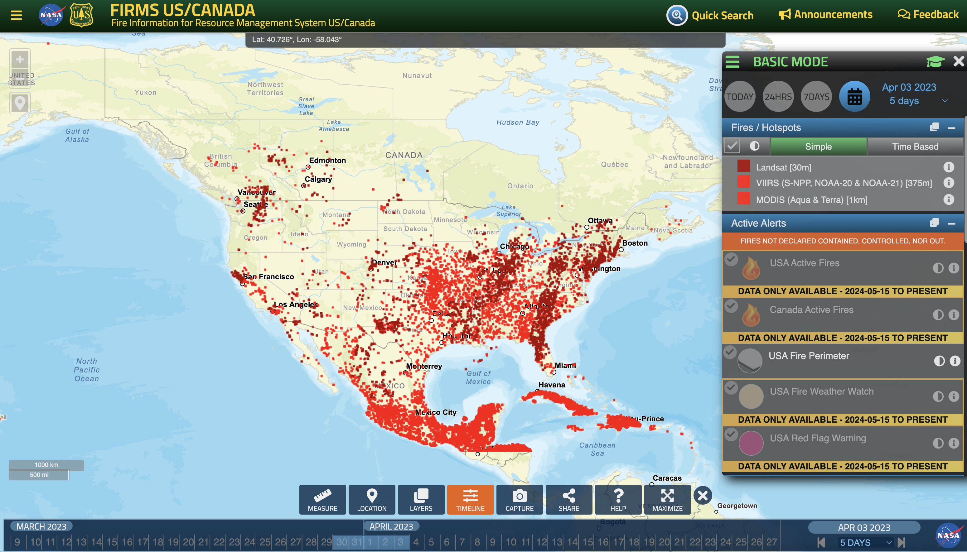
return dsPlotting HYSPLIT back trajectory and compare with NASA firemap
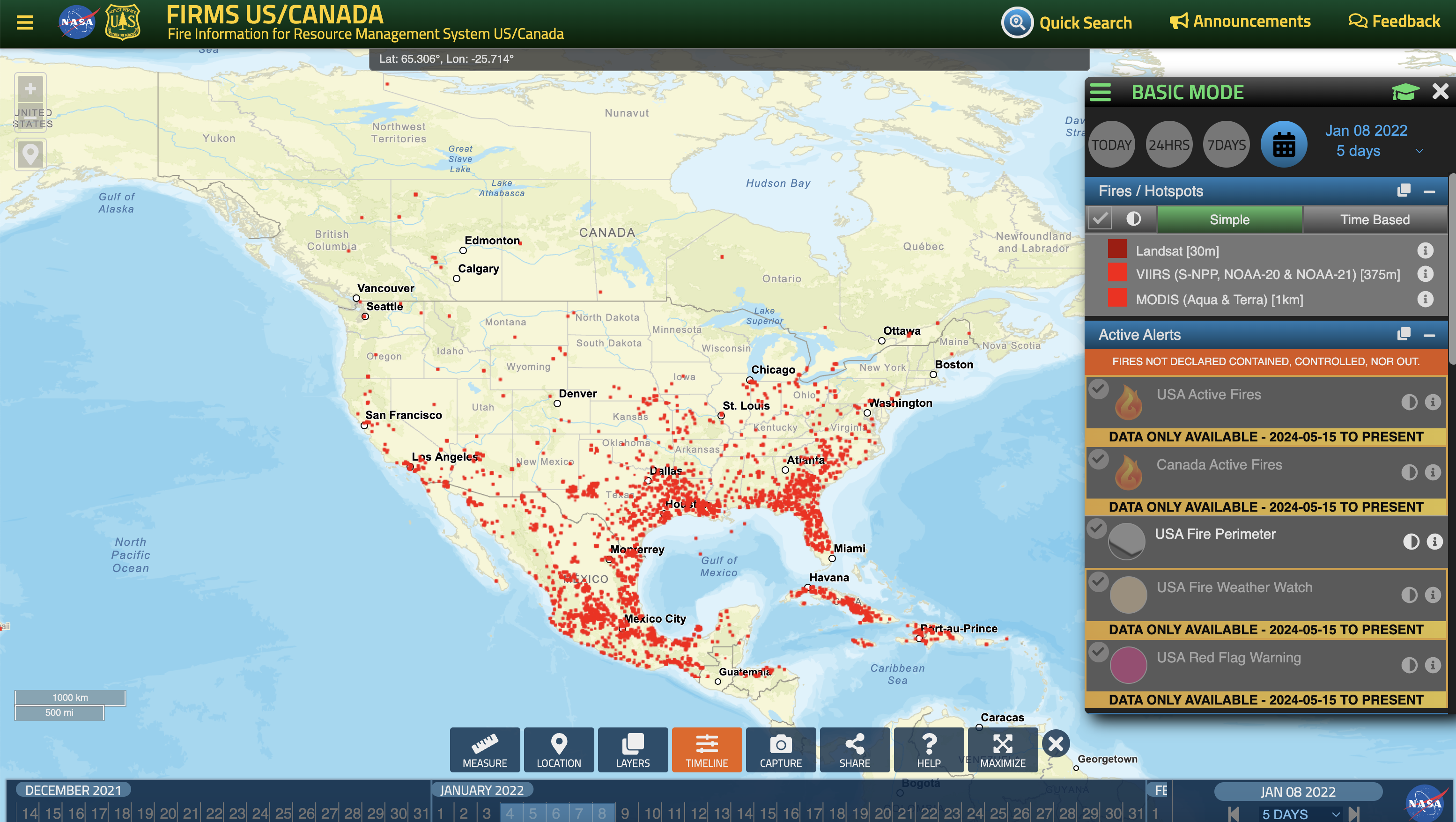
Case 1: Jan 8th, 2022
# Load the data
filename = 'guc_010822.txt'
ds = read_hysplit(filename)

# Use the GeographicPlotDisplay object to make the plot
disp = act.plotting.GeographicPlotDisplay(ds)
ax = disp.geoplot('PRESSURE', cartopy_feature=['STATES', 'OCEAN', 'LAND'], s = 1)
ax.set_xlim([-159, -67])
ax.set_ylim([20, 77])
plt.show()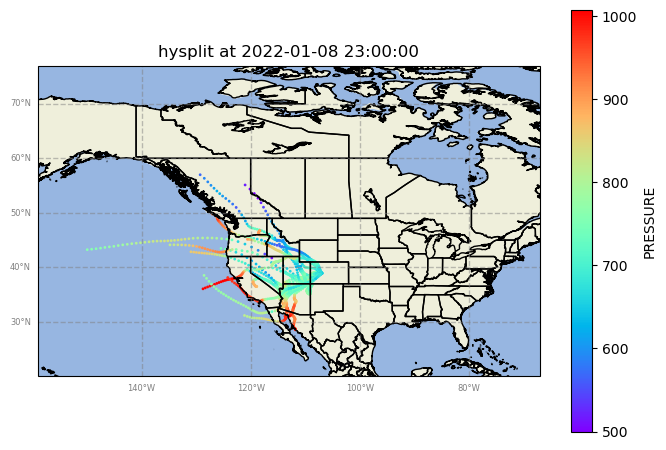
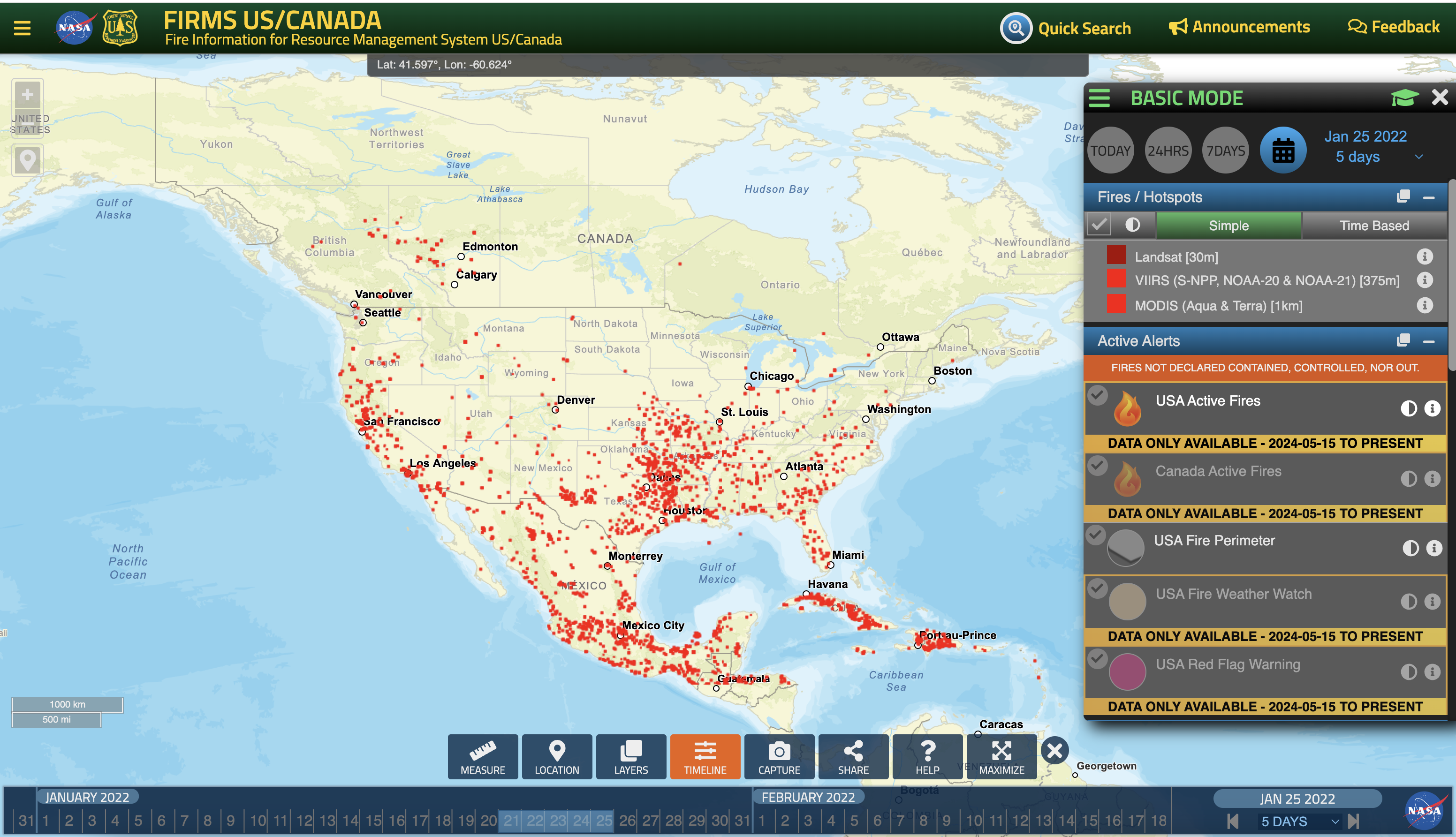
Case 2: Jan 25th, 2022
# Load the data
filename = 'guc_012522.txt'
ds = read_hysplit(filename)

# Use the GeographicPlotDisplay object to make the plot
disp = act.plotting.GeographicPlotDisplay(ds)
ax = disp.geoplot('PRESSURE', cartopy_feature=['STATES', 'OCEAN', 'LAND'], s = 1)
ax.set_xlim([-159, -67])
ax.set_ylim([20, 77])
plt.show()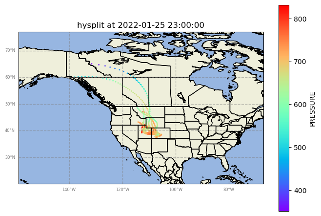
Case 3: Apr 3rd, 2023
# Load the data
filename = 'guc_040323.txt'
ds = read_hysplit(filename)

# Use the GeographicPlotDisplay object to make the plot
disp = act.plotting.GeographicPlotDisplay(ds)
ax = disp.geoplot('PRESSURE', cartopy_feature=['STATES', 'OCEAN', 'LAND'], s = 1)
ax.set_xlim([-159, -67])
ax.set_ylim([20, 77])
plt.show()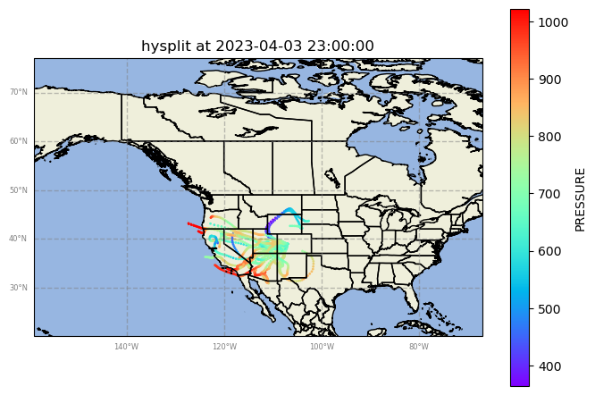
from IPython.display import display, HTML

# Adjust the path to your HTML file accordingly
file_path = "ARM_smps_data.html"

# Read the content of the HTML file
with open(file_path, 'r') as file:
    html_content = file.read()

# Display the HTML content
display(HTML(html_content))
Loading...