Surface temperature comparison

import act
import numpy as np
import xarray as xr
import pandas as pd
import matplotlib.pyplot as plt
from datetime import timedelta
import xwrf
import cmweather
import glob
from bokeh.models.formatters import DatetimeTickFormatter
import hvplot.xarray
import holoviews as hv
hv.extension("bokeh")

# Set your username and token here!
username = '---------'
token = '##########'

# Set the datastream and start/enddates
datastream_snow = 'gucmetM1.b1' # snow depth, also precipitation rate
# datastream_metprep = 'gucmetM1.b1' # surface temperature+precipitation
startdate1 = '2022-01-02'
enddate1 = '2022-01-07'
startdate2 = '2022-01-25'
enddate2 = '2022-01-30'
startdate3 = '2023-04-03'
enddate3 = '2023-04-08'

# wrf: snow depth()
# SNOWNC: ACCUMULATED TOTAL GRID SCALE SNOW AND ICE
# SNOWC: FLAG INDICATING SNOW COVERAGE (1 FOR SNOW COVER)

# Use ACT to easily download the data.  Watch for the data citation!  Show some support
# for ARM's instrument experts and cite their data if you use it in a publication
datasnow1 = act.discovery.download_arm_data(username, token, datastream_snow, startdate1, enddate1)
datasnow2 = act.discovery.download_arm_data(username, token, datastream_snow, startdate2, enddate2)
datasnow3 = act.discovery.download_arm_data(username, token, datastream_snow, startdate3, enddate3)
# datamet = act.discovery.download_arm_data(username, token, datastream_metprep, startdate, enddate)

# Let's read in the data using ACT and check out the data
ds_snow1 = act.io.read_arm_netcdf(datasnow1) # 1-min
ds_snow2 = act.io.read_arm_netcdf(datasnow2) # 1-min
ds_snow3 = act.io.read_arm_netcdf(datasnow3) # 1-min

ds_snow1

ds_snow1["temp_mean"] = ds_snow1["temp_mean"] + 273.15
ds_snow2["temp_mean"] = ds_snow2["temp_mean"] + 273.15
ds_snow3["temp_mean"] = ds_snow3["temp_mean"] + 273.15

ds_snow1["temp_mean"]

variable_snow = "tbrg_precip_total_corr"
variable_temp = "temp_mean"

# Jan 2-7 2022
# Create a plotting display object with 2 plots
display = act.plotting.TimeSeriesDisplay(ds_snow1,subplot_shape=(2,), figsize=(15,10))

# Plot up the variable in the first plot - Surface precipitation corrected (tbrg_precip_total_corr)
display.plot(variable_snow, subplot_index=(0,),day_night_background=True,
             set_title="Control case: Total precipitation")
# display.day_night_background(subplot_index=(0,))

# Plot up the variable in the second plot - Temperature: temp_mean
display.plot(variable_temp, subplot_index=(1,),day_night_background=True,
             set_title="Control case: Surface Temperature")
# display.day_night_background(subplot_index=(1,))
plt.ylabel('(K)')
plt.show()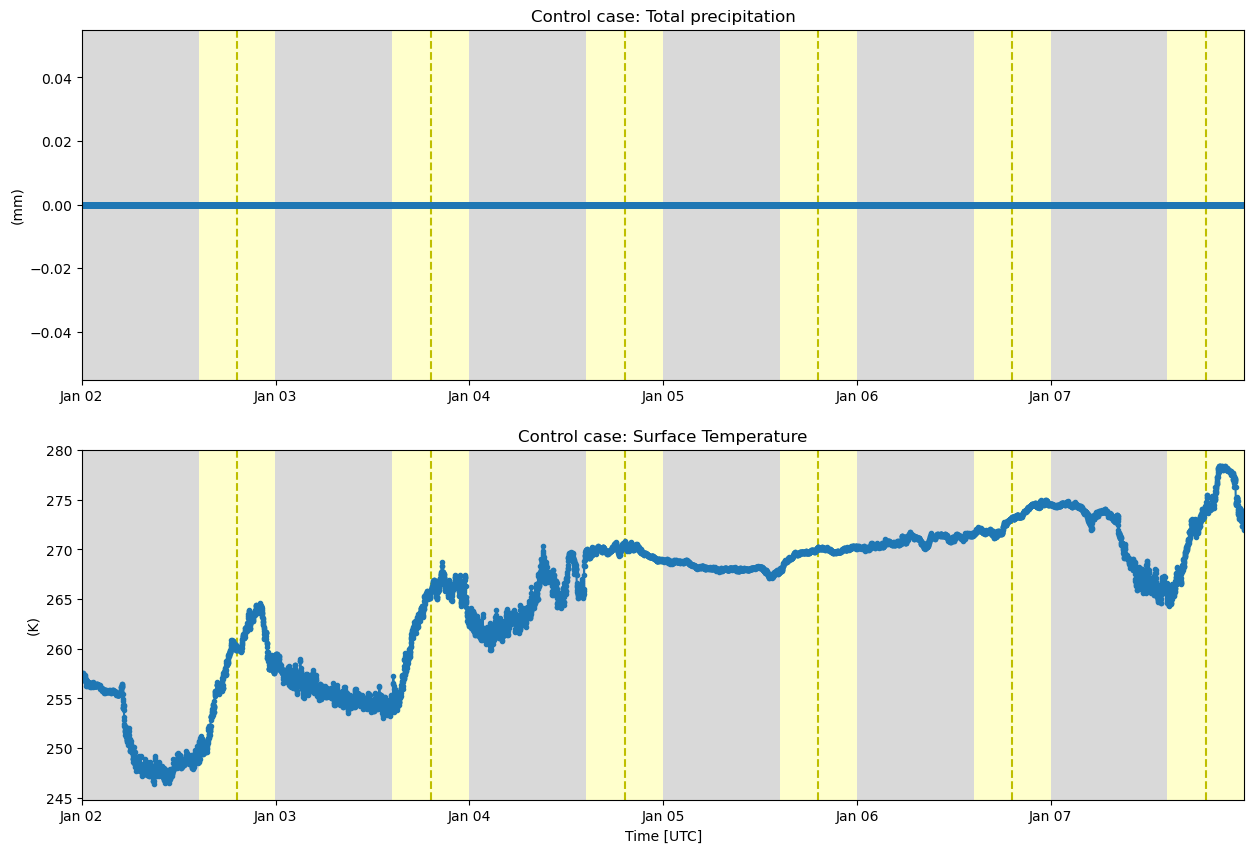 

# Jan 25-30 2022
# Create a plotting display object with 2 plots
display = act.plotting.TimeSeriesDisplay(ds_snow2,subplot_shape=(2,), figsize=(15,10))

# Plot up the variable in the first plot - Surface precipitation corrected (tbrg_precip_total_corr)
display.plot(variable_snow, subplot_index=(0,),day_night_background=True,
             set_title="Black carbon case: Total precipitation")
# display.day_night_background(subplot_index=(0,))

# Plot up the variable in the second plot - Temperature: temp_mean
display.plot(variable_temp, subplot_index=(1,),day_night_background=True,
             set_title="Black carbon case: Surface Temperature")
# display.day_night_background(subplot_index=(1,))

plt.show()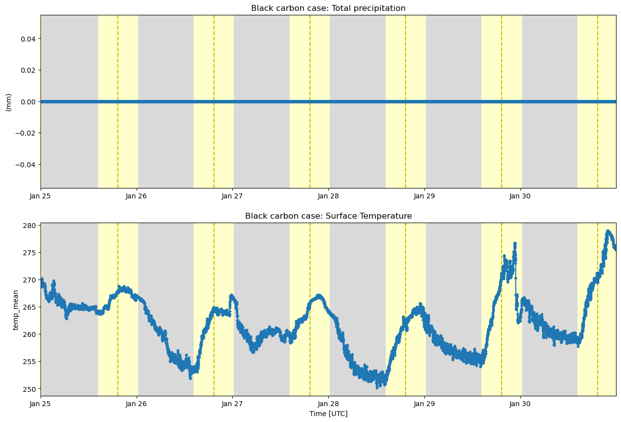 

# Apr 3-8 2022
# Create a plotting display object with 2 plots
display = act.plotting.TimeSeriesDisplay(ds_snow3,subplot_shape=(2,), figsize=(15,10))

# Plot up the variable in the first plot - Surface precipitation corrected (tbrg_precip_total_corr)
display.plot(variable_snow, subplot_index=(0,),day_night_background=True,
             set_title="Dust case: Total precipitation")
# display.day_night_background(subplot_index=(0,))

# Plot up the variable in the second plot - Temperature: temp_mean
display.plot(variable_temp, subplot_index=(1,),day_night_background=True,
             set_title="Dust case: Surface Temperature")
# display.day_night_background(subplot_index=(1,))

plt.show()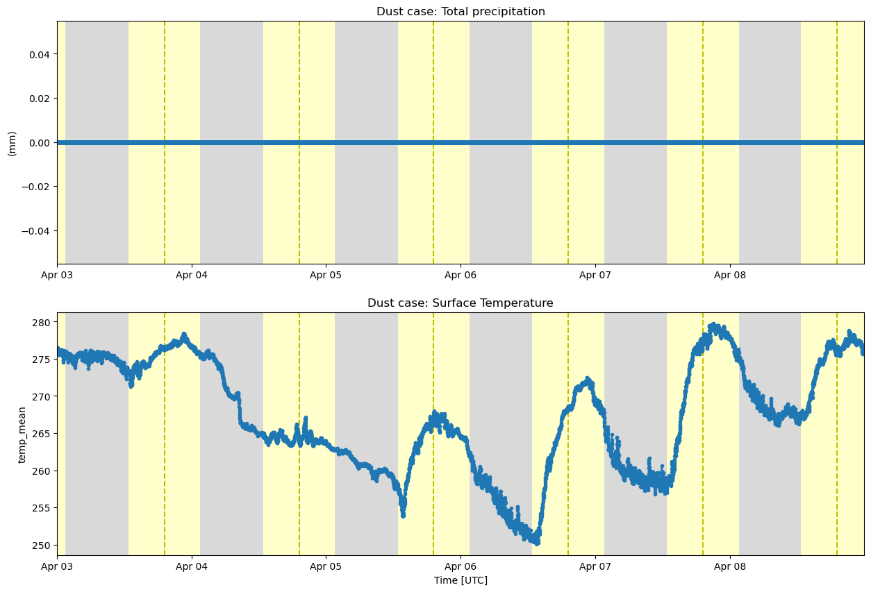 

## WRF
files_ctrl=sorted(glob.glob("/data/home/mqzhang/sail-cookbook/notebooks/downloaded_files/control/*"))
files_bc=sorted(glob.glob("/data/home/mqzhang/sail-cookbook/notebooks/downloaded_files/bc/*"))
files_dust=sorted(glob.glob("/data/home/mqzhang/sail-cookbook/notebooks/downloaded_files/dust/*"))

ds_ctrl = xr.open_mfdataset(files_ctrl,concat_dim="Time",combine="nested").xwrf.postprocess().squeeze()
ds_ctrl

formatter = DatetimeTickFormatter(hours="%d %b %Y \n %H:%M UTC")
ds_ctrl["T2"].mean(dim=['x', 'y']).hvplot(xformatter=formatter)

ds_bc = xr.open_mfdataset(files_bc,concat_dim="Time",combine="nested").xwrf.postprocess().squeeze()
ds_bc

ds_bc["T2"].mean(dim=['x', 'y']).hvplot(xformatter=formatter)

ds_dust = xr.open_mfdataset(files_dust,concat_dim="Time",combine="nested").xwrf.postprocess().squeeze()
ds_dust

ds_dust["T2"].load()
ds_dust["T2"].mean(dim=['x', 'y']).hvplot(x="Time")