Google Cloud CMIP6 Public Data: Basic Python Example

Overview¶

This notebooks shows how to query the Google Cloud CMIP6 catalog and load the data using Python.

Prerequisites¶

Concepts	Importance	Notes
Intro to Xarray	Necessary
Understanding of NetCDF	Helpful	Familiarity with metadata structure

Time to learn: 10 minutes

Imports¶

from matplotlib import pyplot as plt
import numpy as np
import pandas as pd
import xarray as xr
import zarr
import fsspec
import nc_time_axis

%matplotlib inline
plt.rcParams['figure.figsize'] = 12, 6

Browse Catalog¶

The data catatalog is stored as a CSV file. Here we read it with Pandas.

df = pd.read_csv('https://storage.googleapis.com/cmip6/cmip6-zarr-consolidated-stores.csv')
df.head()

The columns of the dataframe correspond to the CMI6 controlled vocabulary.

Here we filter the data to find monthly surface air temperature for historical experiments.

df_ta = df.query("activity_id=='CMIP' & table_id == 'Amon' & variable_id == 'tas' & experiment_id == 'historical'")
df_ta

Now we do further filtering to find just the models from NCAR.

df_ta_ncar = df_ta.query('institution_id == "NCAR"')
df_ta_ncar

Load Data¶

Now we will load a single store using fsspec, zarr, and xarray.

# get the path to a specific zarr store (the first one from the dataframe above)
zstore = df_ta_ncar.zstore.values[-1]
print(zstore)

# create a mutable-mapping-style interface to the store
mapper = fsspec.get_mapper(zstore)

# open it using xarray and zarr
ds = xr.open_zarr(mapper, consolidated=True)
ds

Plot the Data¶

Plot a map from a specific date:

ds.tas.sel(time='1950-01').squeeze().plot()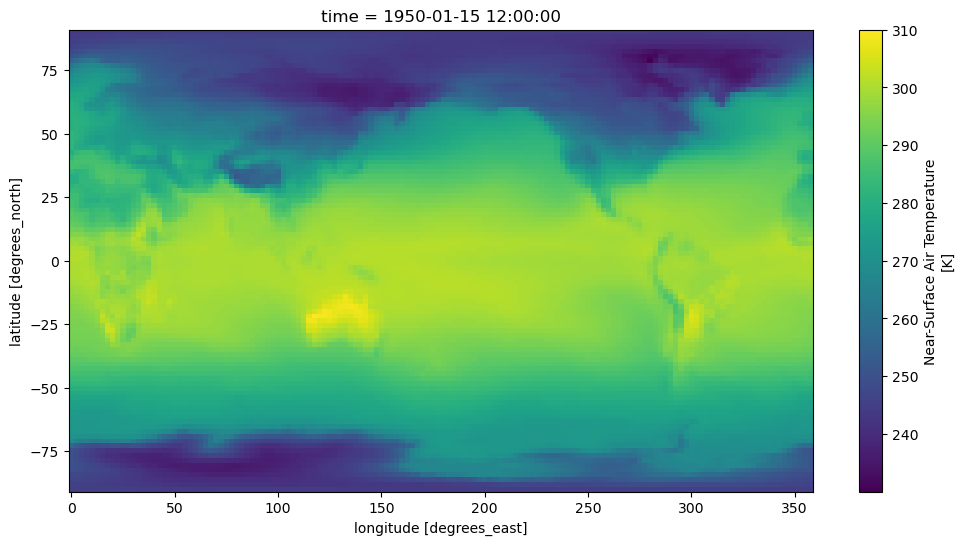

The global mean of a lat-lon field needs to be weighted by the area of each grid cell, which is proportional to the cosine of its latitude.

def global_mean(field):
    weights = np.cos(np.deg2rad(field.lat))
    return field.weighted(weights).mean(dim=['lat', 'lon'])

We can pass all of the temperature data through this function:

ta_timeseries = global_mean(ds.tas)
ta_timeseries

By default the data are loaded lazily, as Dask arrays. Here we trigger computation explicitly.

%time ta_timeseries.load()

ta_timeseries.plot(label='monthly')
ta_timeseries.rolling(time=12).mean().plot(label='12 month rolling mean', color='k')
plt.legend()
plt.grid()
plt.title('Global Mean Surface Air Temperature')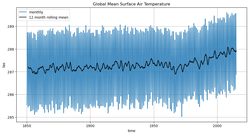

Summary¶

In this notebook, we opened a CESM2 dataset with fsspec and zarr. We calculated and plotted global average surface air temperature.

What’s next?¶

We will open a dataset with ESGF and OPenDAP.

Resources and references¶

Original notebook in the Pangeo Gallery by Henri Drake and Ryan Abernathey

Foundations

Load CMIP6 Data with Intake-ESM

Foundations

Search and Load CMIP6 Data via ESGF/OPeNDAP