ESGF logo Rooki logo Cartopy logo

Demo: Regridding and Plotting with Rooki and Cartopy¶

Overview¶

In this notebook, we demonstrate how to use Rooki to regrid CMIP model data and plot it in Cartopy for two examples:

Regrid two CMIP models onto the same grid
Coarsen the output for one model

Prerequisites¶

Concepts	Importance	Notes
Intro to intake-esgf	Necessary
Intro to Cartopy	Necessary
Using Rooki to access CMIP6 data	Helpful	Familiarity with rooki
Understanding of NetCDF	Helpful	Familiarity with metadata structure

Time to learn: 15 minutes

Imports¶

import os
import intake_esgf

# Run this on the DKRZ node in Germany, using the ESGF1 index node at LLNL
os.environ["ROOK_URL"] = "http://rook.dkrz.de/wps"
intake_esgf.conf.set(indices={"anl-dev": False,
                               "ornl-dev": False,
                               "esgf-node.llnl.gov": True})

import rooki.operators as ops
import matplotlib.pyplot as plt
import matplotlib.colors as mcolors
import cartopy.crs as ccrs
import cartopy.feature as cfeature

import intake_esgf
from intake_esgf import ESGFCatalog
from rooki import rooki
from matplotlib.gridspec import GridSpec
from mpl_toolkits.axes_grid1.inset_locator import inset_axes

Example 1: Regrid two CMIP6 models onto the same grid¶

In this example, we want to compare the historical precipitation output between two CMIP models, CESM2 and CanESM5. Here will will look at the annual mean precipitation for 2010.

Access the desired datasets using intake-esgf and rooki¶

The function and workflow to read in CMPI6 data using intake-esgf and rooki in the next few cells are adapted from intake-esgf-with-rooki.ipynb. Essentially, we use intake-esgf to find the dataset IDs we want and then subset and average them using rooki.

def separate_dataset_id(id_list):
    rooki_id = id_list[0]
    rooki_id = rooki_id.split("|")[0]
    #rooki_id = f"css03_data.{rooki_id}"  # <-- just something you have to know for now :(
    return rooki_id

cat = ESGFCatalog()
cat.search(
        activity_id='CMIP',
        experiment_id=["historical",],
        variable_id=["pr"],
        member_id='r1i1p1f1',
        grid_label='gn',
        table_id="Amon",
        source_id = [ "CESM2", "CanESM5"]
    )

dsets = [separate_dataset_id(dataset) for dataset in list(cat.df.id.values)]
dsets

Subset the data to get the precipitation variable for 2010 and then average by time:

dset_list = [[]]*len(dsets)

for i, dset_id in enumerate(dsets):
    wf = ops.AverageByTime(
        ops.Subset(
            ops.Input('pr', [dset_id]),
            time='2010/2010'
        )
    )

    resp = wf.orchestrate()

    # if it worked, add the dataset to our list
    if resp.ok:
        dset_list[i] = resp.datasets()[0]
        
    # if it failed, tell us why
    else:
        print(resp.status)

Print the dataset list to get an overview of the metadata structure:

print(dset_list)

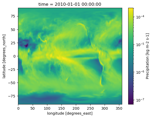
Compare the precipitation data between models¶

First, let’s quickly plot the 2010 annual mean precipitation for each model to see what we’re working with. Since precipitation values vary greatly in magnitude, using a log-normalized colormap makes the data easier to visualize.

for dset in dset_list:
    dset.pr.plot(norm=mcolors.LogNorm())
    plt.show()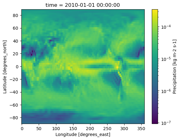

Uncomment and run the following cell. If we try to take the difference outright, it fails!

# pr_diff = dset_list[0].pr - dset_list[1].pr

The models have different grids so we can’t directly subtract the data. We can use the grid attribute to get information on which grid each uses.

print(dset_list[0].grid)
print(dset_list[1].grid)

Regrid the models onto the same grid with Rooki¶

Look at the documentation on the regrid operator to see the available grid types and regrid methods:

rooki.regrid?

Here we’ll do the same process as before to read in and subset the datasets with rooki, but now we regrid using ops.Regrid before averaging over time. In this example, we use method=nearest_s2d to regrid each model onto the target grid using a nearest neighbors method. The target grid is a 1.25° grid, specified by grid='1pt25deg'.

rg_list = [[]]*len(dsets)

for i, dset_id in enumerate(dsets):
    wf = ops.AverageByTime(
        ops.Regrid(
            ops.Subset(
                ops.Input('pr', [dset_id]),
                time='2010/2010'
            ),
            method='nearest_s2d',
            grid='1pt25deg'
        )
    )


    resp = wf.orchestrate()
    
    # if it worked, add the regridded dataset to our list
    if resp.ok:
        rg_list[i] = resp.datasets()[0]
        
    # if it failed, tell us why
    else:
        print(resp.status)

Print the list of regridded datasets to get an overview of the metadata structure. Note how lat and lon are now the same and each dataset has additional attributes, including grid_original and regrid_operation, which all keep track of the regridding operations we just completed.

print(rg_list)

Now they are on the same grid!

print(rg_list[0].grid)
print(rg_list[1].grid)

Quick plot the before and after for each model¶

The plots largely look the same, as they should - with the nearest neighbors method, we are just shifting the precipitation data onto a different grid without averaging between grid cells.

print(dset_list[0].source_id)
for ds in [dset_list[0], rg_list[0]]:
    ds.pr.plot(norm=mcolors.LogNorm())
    plt.show()

print(dset_list[1].source_id)
for ds in [dset_list[1], rg_list[1]]:
    ds.pr.plot(norm=mcolors.LogNorm())
    plt.show()

Take the difference between precipitation datasets and plot it¶

Now that both models are on the same grid, we can subtract the precipitation datasets and plot the difference!

pr_diff = rg_list[0] - rg_list[1]

pr_diff.pr.plot(cmap="bwr")
plt.show()

Plot everything together¶

Plot the regridded precipitation data as well as the difference between models on the same figure. We can use Cartopy to make it pretty. With GridSpec, we can also split up the figure and organize it to use the same colorbar for more than one panel.

# set up figure
fig = plt.figure(figsize=(6, 8))
gs = GridSpec(3, 2, width_ratios=[1, 0.1], hspace=0.2)

# specify the projection
proj = ccrs.Mollweide()

# set up plots for each model
axpr_1 = plt.subplot(gs[0, 0], projection=proj)
axpr_2 = plt.subplot(gs[1, 0], projection=proj)
axdiff = plt.subplot(gs[2, 0], projection=proj)

# axes where the colorbar will go 
axcb_pr = plt.subplot(gs[:2, 1]) 
axcb_diff = plt.subplot(gs[2, 1])
axcb_pr.axis("off")
axcb_diff.axis("off")

# plot the precipitation for both models
for i, ax in enumerate([axpr_1, axpr_2]):
    ds_rg = rg_list[i]
    pcm = ax.pcolormesh(ds_rg.lon, ds_rg.lat, ds_rg.pr.isel(time=0), norm=mcolors.LogNorm(vmin=1e-7, vmax=3e-4),
                         transform=ccrs.PlateCarree()
                       )
    ax.set_title(ds_rg.parent_source_id)
    ax.add_feature(cfeature.COASTLINE)
    
# now plot the difference
pcmd = axdiff.pcolormesh(pr_diff.lon, pr_diff.lat, pr_diff.pr.isel(time=0), cmap="bwr", vmin=-3e-4, vmax=3e-4,
                         transform=ccrs.PlateCarree()
                        )
axdiff.set_title("{a} - {b}".format(a=rg_list[0].parent_source_id, b=rg_list[1].parent_source_id))
axdiff.add_feature(cfeature.COASTLINE)

# set the precipitation colorbar
axcb_pr_ins = inset_axes(axcb_pr, width="50%", height="75%", loc="center")
cbar_pr = plt.colorbar(pcm, cax=axcb_pr_ins, orientation="vertical", extend="both")
cbar_pr.set_label("{n} ({u})".format(n=rg_list[0].pr.long_name, u=rg_list[0].pr.units))

# set the difference colorbar
axcb_diff_ins = inset_axes(axcb_diff, width="50%", height="100%", loc="center")
cbar_diff = plt.colorbar(pcmd, cax=axcb_diff_ins, orientation="vertical", extend="both")
cbar_diff.set_label("Difference ({u})".format(u=pr_diff.pr.units))

plt.show()

Example 2: Coarsen the output for one model¶

We can also use Rooki to regrid the data from one model onto a coarser grid. In this case, it may make more sense to use a conservative regridding method, which will conserve the physical fluxes between grid cells, rather than the nearest neighbors method we used in Example 1.

Get the data using intake-esgf and Rooki again¶

In this example, we’ll look at the annual mean near-surface air temperature for CESM2 in 2010.

cat = ESGFCatalog()
cat.search(
        activity_id='CMIP',
        experiment_id=["historical",],
        variable_id=["tas"],
        member_id='r1i1p1f1',
        grid_label='gn',
        table_id="Amon",
        source_id = [ "CESM2"]
    )

dsets = [separate_dataset_id(dataset) for dataset in list(cat.df.id.values)]
dsets

First, get the dataset with the original grid:

wf = ops.AverageByTime(
    ops.Subset(
        ops.Input('tas', [dsets[0]]),
        time='2010/2010'
    )
)

resp = wf.orchestrate()

if resp.ok:
    ds_og = resp.datasets()[0]
else:
    print(resp.status)

Use the .grid attribute to get information on the native grid:

ds_og.grid

The native grid is 0.9°x1.25°, so let’s try coarsening to a 1.25°x1.25° grid using the conservative method:

wf = ops.AverageByTime(
    ops.Regrid(
        ops.Subset(
            ops.Input('tas', [dsets[0]]),
            time='2010/2010'
        ),
        method='conservative',
        grid='1pt25deg'
    )
)

resp = wf.orchestrate()

if resp.ok:
    ds_125 = resp.datasets()[0]
else:
    print(resp.status)

ds_125.grid

We can also make it even coarser by regridding to a 2.5°x2.5° grid:

wf = ops.AverageByTime(
    ops.Regrid(
        ops.Subset(
            ops.Input('tas', [dsets[0]]),
            time='2010/2010'
        ),
        method='conservative',
        grid='2pt5deg'
    )
)

resp = wf.orchestrate()

if resp.ok:
    ds_25 = resp.datasets()[0]
else:
    print(resp.status)

ds_25.grid

Plot each dataset to look at the coarsened grids¶

Make a quick plot first:

for ds in [ds_og, ds_125, ds_25]:
    ds["tas"].plot()
    plt.show()

Plot the coarsened datsets together using Cartopy¶

Now let’s zoom in on a smaller region, the continental US, to get a clear view of the difference in grid resolution. Here we can also decrease the colorbar limits to better see how the variable tas varies within the smaller region.

# set up the figure
fig = plt.figure(figsize=(6, 8))
gs = GridSpec(3, 2, width_ratios=[1, 0.1], height_ratios=[1, 1, 1], hspace=0.3, wspace=0.2)

# specify the projection
proj = ccrs.PlateCarree()

# set up plot axes
ax1 = plt.subplot(gs[0, 0], projection=proj)
ax2 = plt.subplot(gs[1, 0], projection=proj)
ax3 = plt.subplot(gs[2, 0], projection=proj)
axes_list = [ax1, ax2, ax3]

# set up colorbar axis
axcb = plt.subplot(gs[:, 1])

# loop through each dataset and its corresponding axis
for i, dset in enumerate([ds_og, ds_125, ds_25]):
    plot_ds = dset.tas.isel(time=0)
    ax = axes_list[i]
    pcm = ax.pcolormesh(plot_ds.lon, plot_ds.lat, plot_ds, vmin=270, vmax=302.5, transform=proj)
    
    # add borders and coastlines
    ax.add_feature(cfeature.BORDERS)
    ax.coastlines()
    
    # limit to CONUS for this example
    ax.set_xlim(-130, -60)
    ax.set_ylim(22, 52)
    
    # add grid labels on bottom & left only
    gl = ax.gridlines(color="None", draw_labels=True)
    gl.top_labels = False
    gl.right_labels = False
    
    # label with the regrid type; if it fails, that means it hasn't been regridded
    # (so label with the grid attribute instead)
    try:
        ax.set_title(dset.regrid_operation)
    except:
        ax.set_title(dset.grid)
        
# use the same colorbar for all plots
axcb.axis("off")
axcb_ins = inset_axes(axcb, width="50%", height="75%", loc="center")
cbar = plt.colorbar(pcm, cax=axcb_ins, orientation="vertical", extend="both")
cbar.set_label("{n} ({u})".format(n=plot_ds.long_name, u=plot_ds.units))
        
plt.show()

Summary¶

Rooki offers a quick and easy way to regrid CMIP model data that can be located using intake-esgf. Cartopy lets us easily customize the plot to neatly display the geospatial data.

Resources and references¶

Regridding overview from NCAR, including descriptions of various regridding methods
Rooki regridding example notebook
Rooki documentation
Cartopy logo image source
Rooki logo image source

Workflows

Compute Demo: ENSO nonlinearity index with CMIP6 data

Workflows

Complex Searching with intake and analysing employing xarray