Introduction to `intake-esgf`

Overview

In this tutorial we will discuss the basic functionality of intake-esgf and describe some of what it is doing under the hood. intake-esgf is an intake and intake-esm inspired package under development in ESGF2. Please note that there is a name collison with an existing package in PyPI and conda. You will need to install the package from source.

Prerequisites

Concepts	Importance	Notes
Install Package	Necessary	`pip install git+https://github.com/esgf2-us/intake-esgf`
Familiar with intake-esm	Helpful	Similar interface
Understanding of NetCDF	Helpful	Familiarity with metadata structure

Time to learn: 30 minutes

Imports

from intake_esgf import ESGFCatalog
import matplotlib.pyplot as plt

Populate the Catalog

Unlike intake-esm, our catalogs initialize empty. This is because while intake-esm loads a large file-based database into memory, we are going to populate a catalog by searching one or many index nodes. The ESGFCatalog is configured by default to query a Globus (ElasticSearch) based index which has information about holdings at the (Argonne Leadership Computing Facility (ALCF) only. We will demonstrate how this may be expanded to include other nodes later.

cat = ESGFCatalog()
print(cat)  # <-- nothing to see here yet

Perform a search() to populate the catalog.

cat.search(
    experiment_id="historical",
    source_id="CanESM5",
    frequency="mon",
    variable_id=["gpp", "tas", "pr"],
)
print(cat)

   Searching indices:   0%|          |0/1 [       ?index/s]

   Searching indices: 100%|██████████|1/1 [    1.92s/index]

Summary information for 195 results:
mip_era                                                     [CMIP6]
activity_id                                                  [CMIP]
institution_id                                              [CCCma]
source_id                                                 [CanESM5]
experiment_id                                          [historical]
member_id         [r28i1p2f1, r6i1p2f1, r14i1p1f1, r20i1p2f1, r2...
table_id                                               [Lmon, Amon]
variable_id                                          [gpp, tas, pr]
grid_label                                                     [gn]
dtype: object

The search has populated the catalog where results are stored internally as a pandas dataframe, where the columns are the facets common to ESGF. Printing the catalog will display each column as well as a possibly-truncated list of unique values. We can use these to help narrow down our search. In this case, we neglected to mention a member_id (also known as a variant_label). So we can repeat our search with this additional facet. Note that searches are not cumulative and so we need to repeat the previous facets in this subsequent search. Also, while for the tutorial’s sake we repeat the search here, in your own analysis codes, you could simply edit your previous search.

cat.search(
    experiment_id="historical",
    source_id="CanESM5",
    frequency="mon",
    variable_id=["gpp", "tas", "pr"],
    variant_label="r1i1p1f1",  # addition from the last search
)
print(cat)

   Searching indices: 100%|██████████|1/1 [    1.73s/index]

Summary information for 3 results:
mip_era                  [CMIP6]
activity_id               [CMIP]
institution_id           [CCCma]
source_id              [CanESM5]
experiment_id       [historical]
member_id             [r1i1p1f1]
table_id            [Amon, Lmon]
variable_id       [tas, pr, gpp]
grid_label                  [gn]
dtype: object

Obtaining the datasets

Now we see that our search has located 3 datasets and thus we are ready to load these into memory. Like intake-esm, the catalog will generate a dictionary of xarray datasets. Internally, the catalog is again communicating with the index node and requesting file information. This includes which file or files are part of the datasets, their local paths, download locations, and verification information. We then try to make an optimal decision in getting the data to you as quickly as we can.

If you are running on a resource with direct access to the ESGF holdings (such a Jupyter notebook on nimbus.llnl.gov), then we check if the dataset files are locally available. We have a handful of locations built-in to intake-esgf but you can also set a location manually with cat.set_esgf_data_root().
If a dataset has associated files that have been previously downloaded into the local cache, then we will load these files into memory.
If no direct file access is found, then we will queue the dataset files for download. File downloads will occur in parallel from the locations which provide you the fastest transfer speeds. Initially we will randomize the download locations, but as you use intake-esgf, we keep track of which servers provide you fastest transfer speeds and future downloads will prefer these locations. Once downloaded, we check file validity, and load into xarray containers.

dsd = cat.to_dataset_dict()

 Obtaining file info:   0%|          |0/3 [     ?dataset/s]

 Obtaining file info: 100%|██████████|3/3 [  1.23s/dataset]
Adding cell measures: 100%|██████████|3/3 [  3.00s/dataset]

You will notice that progress bars inform you that file information is being obtained and that downloads are taking place. As files are downloaded, they are placed into a local cache in ${HOME}/.esgf in a directory structure that mirrors that of the remote storage. For future analysis which uses these datasets, intake-esgf will first check this cache to see if a file already exists and use it instead of re-downloading. Then it returns a dictionary whose keys are by default the minimal set of facets to uniquely describe a dataset in the current search.

print(dsd.keys())

dict_keys(['Amon.tas', 'Amon.pr', 'Lmon.gpp'])

During the download process, you may have also noticed that a progress bar informed you that we were adding cell measures. If you have worked with ESGF data before, you know that cell measure information like areacella is needed to take proper area-weighted means/summations. Yet many times, model centers have not uploaded this information uniformly in all submissions. We perform a search for each dataset being placed in the dataset dictionary, progressively dropping dataset facets to find, if possible, the cell measures that are closest to the dataset being downloaded. Sometimes they are simply in another variant_label, but other times they could be in a different activity_id. No matter where they are, we find them for you and add them by default (disable with to_dataset_dict(add_measures=False)).

We determine which measures need downloaded by looking in the dataset attributes. Since tas is an atmospheric variable, we will see that its cell_measures = 'area: areacella'. If you print this variable you will see that measure has been added.

However, for gpp we also need the land fractions, which is detected by the presence of area: where land in the cell_methods. You will notice that both areacella and sftlf are added to Lmon.gpp.

Simple Plotting

fig, axs = plt.subplots(figsize=(6, 12), nrows=3)

# temperature
ds = dsd["Amon.tas"]["tas"].mean(dim="time") - 273.15  # to [C]
ds.plot(ax=axs[0], cmap="bwr", vmin=-40, vmax=40, cbar_kwargs={"label": "tas [C]"})

# precipitation
ds = dsd["Amon.pr"]["pr"].mean(dim="time") * 86400 / 999.8 * 1000  # to [mm d-1]
ds.plot(ax=axs[1], cmap="Blues", vmax=10, cbar_kwargs={"label": "pr [mm d-1]"})

# gross primary productivty
ds = dsd["Lmon.gpp"]["gpp"].mean(dim="time") * 86400 * 1000  # to [g m-2 d-1]
ds.plot(ax=axs[2], cmap="Greens", cbar_kwargs={"label": "gpp [g m-2 d-1]"});

../_images/861a5a7c186719b305d5b20401dcafd868cd5218a418bc67567844bed06ea8a9.png

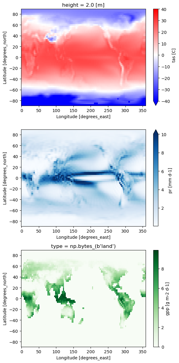
Summary

intake-esgf becomes the way that you download or locate data as well as load it into memory. It is a full specification of what your analysis is about and makes your script portable to other machines or even in use with serverside computing. We are actively developing this codebase. Let us know what other features you would like to see.

Introduction to intake-esgf