### List of files to download for testing
urls2dwn = [ 
  'https://noaa-goes16.s3.amazonaws.com/ABI-L1b-RadF/2021/099/23/OR_ABI-L1b-RadF-M6C01_G16_s20210992350171_e20210992359479_c20210992359525.nc',
  'https://noaa-goes16.s3.amazonaws.com/ABI-L1b-RadF/2021/099/23/OR_ABI-L1b-RadF-M6C02_G16_s20210992350171_e20210992359479_c20210992359522.nc',
  'https://noaa-goes16.s3.amazonaws.com/ABI-L1b-RadF/2021/099/23/OR_ABI-L1b-RadF-M6C03_G16_s20210992350171_e20210992359479_c20210992359530.nc',
  'https://noaa-goes16.s3.amazonaws.com/ABI-L1b-RadF/2021/099/23/OR_ABI-L1b-RadF-M6C04_G16_s20210992350171_e20210992359479_c20210992359514.nc',
  'https://noaa-goes16.s3.amazonaws.com/ABI-L1b-RadF/2021/099/23/OR_ABI-L1b-RadF-M6C05_G16_s20210992350171_e20210992359479_c20210992359533.nc',
  'https://noaa-goes16.s3.amazonaws.com/ABI-L1b-RadF/2021/099/23/OR_ABI-L1b-RadF-M6C06_G16_s20210992350171_e20210992359484_c20210992359528.nc',
  'https://noaa-goes16.s3.amazonaws.com/ABI-L1b-RadF/2021/099/23/OR_ABI-L1b-RadF-M6C07_G16_s20210992350171_e20210992359490_c20210992359539.nc',
  'https://noaa-goes16.s3.amazonaws.com/ABI-L1b-RadF/2021/099/23/OR_ABI-L1b-RadF-M6C08_G16_s20210992350171_e20210992359479_c20210992359535.nc',
  'https://noaa-goes16.s3.amazonaws.com/ABI-L1b-RadF/2021/099/23/OR_ABI-L1b-RadF-M6C09_G16_s20210992350171_e20210992359484_c20210992359551.nc',
  'https://noaa-goes16.s3.amazonaws.com/ABI-L1b-RadF/2021/099/23/OR_ABI-L1b-RadF-M6C10_G16_s20210992350171_e20210992359490_c20210992359536.nc',
  'https://noaa-goes16.s3.amazonaws.com/ABI-L1b-RadF/2021/099/23/OR_ABI-L1b-RadF-M6C11_G16_s20210992350171_e20210992359479_c20210992359545.nc',
  'https://noaa-goes16.s3.amazonaws.com/ABI-L1b-RadF/2021/099/23/OR_ABI-L1b-RadF-M6C12_G16_s20210992350171_e20210992359484_c20210992359539.nc',
  'https://noaa-goes16.s3.amazonaws.com/ABI-L1b-RadF/2021/099/23/OR_ABI-L1b-RadF-M6C13_G16_s20210992350171_e20210992359490_c20210992359555.nc',
  'https://noaa-goes16.s3.amazonaws.com/ABI-L1b-RadF/2021/099/23/OR_ABI-L1b-RadF-M6C14_G16_s20210992350171_e20210992359479_c20210992359547.nc',
  'https://noaa-goes16.s3.amazonaws.com/ABI-L1b-RadF/2021/099/23/OR_ABI-L1b-RadF-M6C15_G16_s20210992350171_e20210992359484_c20210992359557.nc',
  'https://noaa-goes16.s3.amazonaws.com/ABI-L1b-RadF/2021/099/23/OR_ABI-L1b-RadF-M6C16_G16_s20210992350171_e20210992359490_c20210992359542.nc']

import requests
import os

# Specify the local directory where you want to save the files.
# local_directory = input("Enter the path to the download folder: ")
local_directory = "Output_data/ABI-L1b-RadF/s20210992350171"
# Ensure that the local directory exists; create it if it doesn't.
os.makedirs(local_directory, exist_ok=True)

# Iterate through the URLs and download files.
for urld in urls2dwn:
    # Extract the filename from the URL.
    ntw = urld.split('/')[-1]
    
    # Construct the complete path to save the file in the local directory.
    file_path = os.path.join(local_directory, ntw)
    
    # Send an HTTP GET request to the URL.
    resp = requests.get(urld)
    
    # Check if the response is successful (status code 200).
    if resp.status_code == 200:
        # Write the content to the file in binary mode.
        with open(file_path, "wb") as file:
            file.write(resp.content)
        print(f"File '{ntw}' downloaded and saved to '{local_directory}'.")
    else:
        print(f"Failed to download '{ntw}' from the URL: {urld}")

# To stop extraneous warning messages from clogging the notebook output, 
# import the warnings module and set it to ignore all warnings.
import warnings
warnings.filterwarnings('ignore')

# Scene is a representation of satellite data that enables functions such as data reading, 
# data resampling, data compositing, and data saving.
from satpy.scene import Scene
# This line imports the debug_on function from the satpy.utils module, which is used to enable detailed 
# debug logging in Satpy. This can be helpful for troubleshooting and understanding the internal workings of Satpy processes.
from satpy.utils import debug_on

# Importing datetime for date and time operations. Processing time-stamped satellite data 
# is necessary for accurate time-based operations and analysis.
from datetime import datetime

# Using glob allows for efficient and flexible file handling, especially when dealing with 
# large datasets typically generated by geostationary satellites.
from glob import glob

# The magic command '%matplotlib inline' configures the Jupyter Notebook to display plots directly below the code cells.
# This setting is essential for interactive data visualization, especially when plotting data from geostationary satellites.
%matplotlib inline

sat_files = glob("./Output_data/ABI-L1b-RadF/s20210992350171/*")
sat_files

# Create a Scene object named 'scn' by providing a list of filenames obtained from 'fGRl1b'.
# The Scene object is a core part of the Satpy library, which organizes and manages multiple data sources typically from satellite observations.
scn = Scene(filenames = sat_files, reader = 'abi_l1b')

# Retrieve the names of all datasets available in the 'scn' object, which represent various satellite data channels.
# This information is crucial for understanding what types of data are available for analysis, such as different spectral bands and derived products.
dataset_names = scn.all_dataset_names()

# Output the list of dataset names. This is useful for educational purposes to show students the variety of data that can be processed
# and to select specific datasets for further analysis in practical exercises.
print(dataset_names)

# Load multiple datasets using a list comprehension to generate dataset names.
# List comprehensions provide a concise way to create lists based on existing lists or ranges.
# In this case, we generate names for the datasets 'C01' to 'C16', which are typical channel identifiers in satellite data.
scn.load([f'C{x:02d}' for x in range(1, 17)])

# Explanation of the list comprehension:
# [f'C{x:02d}' for x in range(1, 17)] creates a list of strings from 'C01' to 'C16'.
# 'f' before the string starts an f-string, allowing us to insert variables directly into the string.
# '{x:02d}' formats the number 'x' as a two-digit decimal, padding with zeros if necessary.

# The 'scn.load' function is then used to load these specific datasets into the Scene object.
# Loading multiple channels like this is common in the analysis of satellite imagery,
# where each channel can represent different spectral bands and contain different types of environmental information.

# The method 'available_composite_names' is called on the 'scn' object.
# This method retrieves a list of all the composite images that can be created using the loaded data channels.
# Composite images are made by combining multiple data channels to enhance the visualization and interpretation of satellite data.
# This feature is particularly useful in the study of geostationary satellites, as it allows for more detailed and informative visual representations of atmospheric phenomena.

# Retrieve and print the list of available composite names, providing a crucial insight into the data visualization capabilities.
print(scn.available_composite_names())

# Assign the dataset name 'airmass' to the variable 'rgb_im'.
# This variable naming provides clarity when referencing the dataset in multiple places, 
# ensuring consistency and reducing the likelihood of errors in dataset identification.
rgb_im = 'airmass'

# Load the dataset named 'airmass' using the 'scn.load' method.
# The 'airmass' composite is particularly useful in meteorology as it combines several spectral bands to highlight features like dust, ash, and water vapor,
# making it easier to analyze atmospheric conditions from geostationary satellite data.
scn.load([rgb_im])

# Display the loaded 'airmass' dataset using 'scn.show'.
# This method visualizes the specified dataset, allowing students to see the practical application of satellite data composites 
# and understand their relevance in real-world atmospheric monitoring and analysis.
scn.show(rgb_im)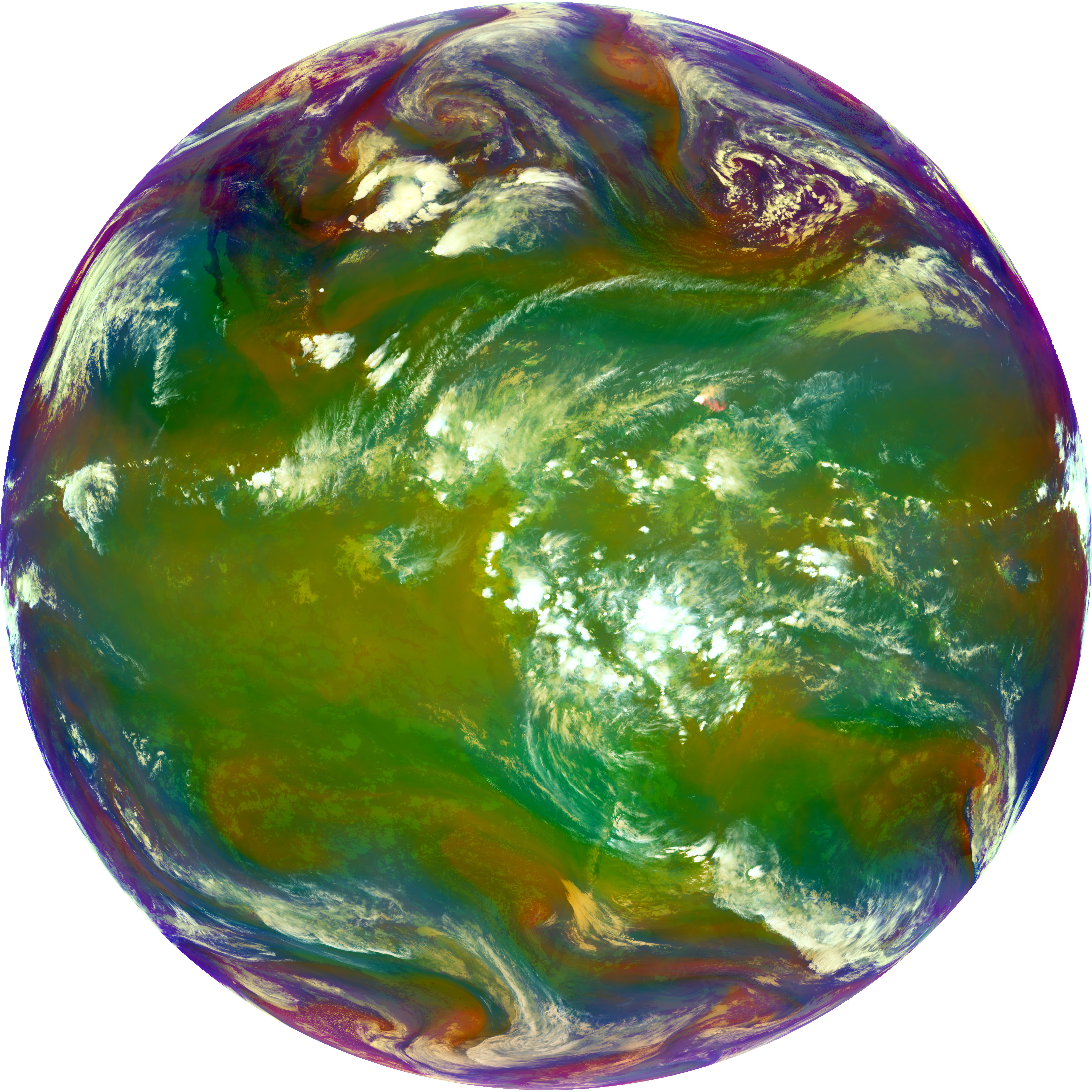

# Access the dataset named 'airmass' from the 'scn' object using the previously defined variable 'rgb_im'.
# The variable 'rgb_im' holds the string 'airmass', which acts as a key to retrieve the corresponding dataset from the Scene object.
# This operation is critical in satellite data processing as it allows for direct manipulation and analysis of specific datasets.
result = scn[rgb_im]

# The retrieved dataset can then be used for further analysis, visualization, or processing.
# It's important for students to understand how to efficiently access and work with specific datasets within a complex data structure.
result

# Retrieve the keys (dataset names) available in the 'scn' object
# This function lists all dataset identifiers stored in the Scene object, each represented as a DataID object.
keys = scn.keys()

# The output is a list of DataID objects, each encapsulating the metadata for a different satellite data channel or composite.
# These DataIDs include crucial information such as:
# - name: The identifier of the dataset, like 'C01', 'C02', ..., 'C16', 'airmass'.
# - wavelength: A WavelengthRange object indicating the spectral range each channel covers, important for identifying the type of observations (e.g., visible, infrared).
# - resolution: The spatial resolution of the data in meters, which affects the detail level visible in the imagery.
# - calibration: The type of calibration applied to the data, which could be reflectance or brightness temperature, impacting how the data should be interpreted.
# - modifiers: Any additional processing applied to the data channel.

# Print the keys to show the available datasets and their properties, aiding in understanding the capabilities and focus areas of the satellite instrument.
keys

# Access the area information associated with the 'C13' dataset in the 'scn' object.
# The area property of a dataset within a Scene object provides geographical and geometric details about the satellite data.
# This includes information such as the projection, extent, resolution, and size of the dataset, which are crucial for spatial analysis.

# For the 'C13' dataset, which typically represents an infrared channel on geostationary satellites, 
# understanding its area is essential for accurately interpreting spatial phenomena observed in the imagery, such as cloud formations or surface temperatures.
area_info = scn["C13"].area

# Print the area information to provide insights into the spatial characteristics of the 'C13' dataset.
# This information supports tasks such as mapping, data integration with other geospatial datasets, and more precise environmental monitoring.
area_info

# Access the area definition information for the 'C01' dataset in the 'scn' object.
# The 'area' property of a dataset provides detailed geographic and geometric information about where the satellite data was collected.
# This includes details such as projection type, coordinate reference system, image extent, and pixel resolution.

# The 'C01' channel, which often captures data in a visible light wavelength (approximately 0.47 µm),
# provides high-resolution imagery useful for detailed visual inspections of cloud cover, surface features, and atmospheric conditions.
area_info = scn["C01"].area

# Print the area information to give insights into the geographic scope and detail level of the 'C01' dataset.
# This is crucial for applications such as mapping, tracking environmental changes, and integrating satellite data with other geographic information systems (GIS).
area_info

# Access the area definition information for the 'C02' dataset in the 'scn' object.
# The 'area' property of a dataset provides crucial geographic and geometric information about the data's capture region.
# This includes the projection type, coordinate system, extent of the image, and pixel resolution.

# The 'C02' channel is typically in the visible spectrum (centered around 0.64 µm), offering detailed imagery suitable for analyzing surface features,
# cloud formations, and atmospheric phenomena. This channel is instrumental in meteorological analysis and environmental monitoring.
area_info = scn["C02"].area

# Print the area information to provide insights into the geographic scope and resolution of the 'C02' dataset.
# Understanding this information is vital for accurate mapping, environmental monitoring, and integration with other geospatial data sources.
area_info

# Load the "natural_color" dataset using the 'scn.load' method.
# The "natural_color" composite is a popular visual representation that combines multiple spectral bands
# to produce an image that approximates what the human eye would see from space. 
# This is particularly useful in earth observation for visualizing land cover, water bodies, and other natural features.

# The composite typically leverages red, green, and blue spectral bands to enhance the clarity and detail of the image,
# which makes it ideal for presentations, educational purposes, and initial visual assessments in environmental studies.
scn.load(["natural_color"])

# This step is crucial for subsequent visualization and analysis tasks, as it prepares the data for easy interpretation and application.

# Get the area definition of the "C13" dataset from the 'scn' object.
# The 'area' property contains critical geographic and geometric information, including projection, extent, and resolution,
# which is essential for accurate geographic referencing in satellite imagery analysis.
rs = scn["C13"].area

# Resample the scene to the specified area definition.
# Resampling is a critical process in satellite data handling, allowing datasets to be standardized to a common spatial grid.
# This standardization is necessary for accurate comparison and integration of different data types and sources.

# Here, 'scn.resample(rs)' adjusts all data in the scene to match the area definition of the 'C13' dataset.
# This is particularly useful when preparing data for detailed analysis or visualization,
# ensuring consistency across different datasets within the same scene.
lscn = scn.resample(rs)

# The resulting 'lscn' is a new Scene object containing all the original data,
# but now aligned to the same geographic grid as the 'C13' dataset.
# This uniformity is crucial for subsequent processing steps, such as creating composites or conducting multi-temporal analysis.

# Load the "natural_color" dataset for the resampled scene.
# The 'natural_color' composite is designed to mimic the colors visible to the human eye by combining specific spectral bands.
# Loading this dataset into the resampled scene ('lscn') ensures that the data is properly aligned and standardized across the same geographic area.

lscn.load(["natural_color"])

# Display the "natural_color" dataset.
# This step involves visualizing the loaded dataset using the 'show' method, which renders the satellite image according to the data's true or natural color representation.
# Visualizing data in this way is particularly useful for presentations and educational purposes, providing a realistic view of earth's features such as vegetation, water bodies, and urban areas.

# lscn.show("natural_color")

# This visualization step is crucial for analyzing environmental and atmospheric conditions,
# as it allows observers to easily identify and assess visible features without the need for specialized image interpretation skills.

# Crop the resampled scene (lscn) to a specific geographic region defined by latitude and longitude bounds.
# The bounds are given as a tuple in the format (lon_min, lat_min, lon_max, lat_max).
# This operation is useful for focusing the analysis on a particular area of interest, reducing data volume and enhancing processing efficiency.
scn_c1 = lscn.crop(ll_bbox=(-65.7, 10.7, -55.9, 20.1))

# Display the "C13" dataset from the cropped scene (scn_c1).
# The "C13" channel typically represents an infrared wavelength used for observing cloud structure and surface temperature,
# crucial for meteorological studies and weather forecasting.
# Displaying this dataset allows for detailed observation of atmospheric conditions within the specified geographic area.

### Uncomment to show it
#scn_c1.show("C13")

# Visualizing specific channels like "C13" in defined geographic regions helps in targeted analysis,
# such as monitoring storm development or evaluating climate patterns in detail.
# This capability is particularly valuable in educational settings for demonstrating real-world applications of satellite data analysis.

# Load the "ash" dataset from the cropped scene (scn_c1).
# The "ash" composite is specifically designed to detect and visualize volcanic ash in the atmosphere using satellite data.
# This dataset is crucial for monitoring volcanic activity and assessing the distribution and movement of ash clouds,
# which can have significant impacts on air quality and aviation safety.
scn_c1.load(['ash'])

# Display the "ash" dataset from the cropped scene (scn_c1).
# Displaying this dataset allows for visual assessment of ash presence within the specified geographic area.
# The visualization is particularly useful in educational and operational settings for demonstrating how satellite data can be applied to real-world environmental challenges.

### Uncomment to show it
# scn_c1.show('ash')

# This step not only aids in the educational demonstration of satellite capabilities but also provides practical insights into the management of natural disasters.
# Such visualizations are essential tools in emergency response planning and environmental monitoring.

# Load the "so2" dataset from the cropped scene (scn_c1).
# The "so2" dataset is designed to detect sulfur dioxide (SO2) concentrations in the atmosphere using satellite data.
# SO2 is a significant volcanic gas and industrial pollutant, making this dataset crucial for monitoring air quality and volcanic activity.
scn_c1.load(['so2'])

# Display the "so2" dataset from the cropped scene (scn_c1).
# Displaying this dataset allows for a visual assessment of SO2 distribution within the specified geographic area.
# The visualization helps in understanding the spatial extent and concentration of sulfur dioxide, which is essential for both environmental and public health assessments.

### Uncomment to show it
# scn_c1.show('so2')

# This step not only aids in the educational demonstration of how satellite imagery can be utilized to monitor environmental pollutants but also provides practical insights into the management of air quality.
# Such visualizations are valuable tools for researchers, policymakers, and educators in understanding and addressing atmospheric pollution.