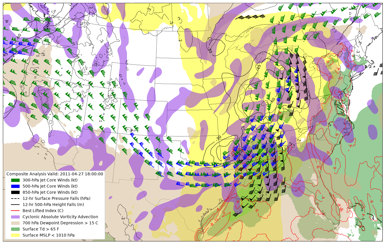
Create a Miller Composite chart based on Miller 1972 in Python with MetPy and Matplotlib.
from datetime import datetime, timedelta

import cartopy.crs as ccrs
import cartopy.feature as cfeature
import matplotlib.lines as lines
import matplotlib.patches as mpatches
import matplotlib.pyplot as plt
import metpy.calc as mpcalc
import numpy as np
import numpy.ma as ma

from metpy.units import units
from netCDF4 import num2date
from scipy.ndimage import gaussian_filter
from siphon.catalog import TDSCatalog
from xarray.backends import NetCDF4DataStore
import xarray as xr
Get the data
This example will use data from the North American Mesoscale Model Analysis for 18 UTC 27 April 2011.
# Specify our date/time of product desired
dt = datetime(2011, 4, 27, 18)

# Construct the URL for our THREDDS Data Server Catalog,
# and access our desired dataset within via NCSS
base_url = 'https://www.ncei.noaa.gov/thredds/catalog/model-namanl-old/'
cat = TDSCatalog(f'{base_url}{dt:%Y%m}/{dt:%Y%m%d}/catalog.xml')
ncss = cat.datasets[f'namanl_218_{dt:%Y%m%d}_{dt:%H}00_000.grb'].subset()

# Create our NCSS query with desired specifications
query = ncss.query()
query.all_times()
query.add_lonlat()
query.lonlat_box(-135, -60, 15, 65)
query.variables('Geopotential_height_isobaric',
                'u-component_of_wind_isobaric',
                'v-component_of_wind_isobaric',
                'Temperature_isobaric',
                'Relative_humidity_isobaric',
                'Best_4_layer_lifted_index_layer_between_two_pressure_'
                'difference_from_ground_layer',
                'Absolute_vorticity_isobaric',
                'Pressure_reduced_to_MSL_msl',
                'Dew_point_temperature_height_above_ground')

# Obtain the data we've queried for
data_18z = ncss.get_data(query)

# Make into an xarray Dataset object
ds_18z = xr.open_dataset(NetCDF4DataStore(data_18z)).metpy.parse_cf()

# Assign variable names to collected data
lat = ds_18z.lat
lon = ds_18z.lon

# Create more useable times for output
times = ds_18z.Geopotential_height_isobaric.metpy.time.squeeze()
vtimes = times.values.astype('datetime64[ms]').astype('O')

temps = ds_18z.Temperature_isobaric.squeeze()
uwnd = ds_18z['u-component_of_wind_isobaric'].squeeze()
vwnd = ds_18z['v-component_of_wind_isobaric'].squeeze()
hgt = ds_18z.Geopotential_height_isobaric.squeeze()
relh = ds_18z.Relative_humidity_isobaric.squeeze()
lifted_index = ds_18z['Best_4_layer_lifted_index_layer_between_two_'
                      'pressure_difference_from_ground_layer'].squeeze()
Td_sfc = ds_18z.Dew_point_temperature_height_above_ground.squeeze()
avor = ds_18z.Absolute_vorticity_isobaric.squeeze()
pmsl = ds_18z.Pressure_reduced_to_MSL_msl.squeeze()
Repeat the above process to query for the analysis from 12 hours earlier (06 UTC) to calculate pressure falls and height change.
td = timedelta(hours=12)

ncss_06z = cat.datasets[f'namanl_218_{dt:%Y%m%d}_{dt-td:%H}00_000.grb'].subset()

query = ncss_06z.query()
query.all_times()
query.add_lonlat()
query.lonlat_box(-135, -60, 15, 65)
query.variables('Geopotential_height_isobaric',
                'Pressure_reduced_to_MSL_msl')

# Actually getting the data
data_06z = ncss_06z.get_data(query)

# Make into an xarray Dataset object
ds_06z = xr.open_dataset(NetCDF4DataStore(data_06z)).metpy.parse_cf()

hgt_06z = ds_06z.Geopotential_height_isobaric.squeeze()
pmsl_06z = ds_06z.Pressure_reduced_to_MSL_msl.squeeze()
Subset the Data
With the data pulled in, we will now subset to the specific levels desired
# 300 hPa
u_300 = uwnd.metpy.sel(vertical=300*units.hPa).metpy.convert_units('kt').squeeze()
v_300 = vwnd.metpy.sel(vertical=300*units.hPa).metpy.convert_units('kt').squeeze()

# 500 hPa
avor_500 = avor.metpy.sel(vertical=500*units.hPa)
u_500 = uwnd.metpy.sel(vertical=500*units.hPa).metpy.convert_units('kt').squeeze()
v_500 = vwnd.metpy.sel(vertical=500*units.hPa).metpy.convert_units('kt').squeeze()
hgt_500 = hgt.metpy.sel(vertical=500*units.hPa).squeeze()
hgt_500_06z = hgt_06z.metpy.sel(vertical=500*units.hPa).squeeze()

# 700 hPa
tmp_700 = temps.metpy.sel(vertical=700*units.hPa).metpy.convert_units('degC').squeeze()
rh_700 = relh.metpy.sel(vertical=700*units.hPa).squeeze()

# 850 hPa
u_850 = uwnd.metpy.sel(vertical=850*units.hPa).metpy.convert_units('kt').squeeze()
v_850 = vwnd.metpy.sel(vertical=850*units.hPa).metpy.convert_units('kt').squeeze()
Prepare Variables for Plotting
With the data queried and subset, we will make any needed calculations in preparation for plotting.
The following fields should be plotted:
500-hPa cyclonic vorticity advection
Surface-based Lifted Index
The axis of the 300-hPa, 500-hPa, and 850-hPa jets
Surface dewpoint
700-hPa dewpoint depression
12-hr surface pressure falls and 500-hPa height changes
# 500 hPa CVA
vort_adv_500 = mpcalc.advection(avor_500, u_500, v_500,) * 1e9
vort_adv_500_smooth = gaussian_filter(vort_adv_500, 4)
/tmp/ipykernel_4405/1703524492.py:2: UserWarning: Vertical dimension number not found. Defaulting to (..., Z, Y, X) order.
vort_adv_500 = mpcalc.advection(avor_500, u_500, v_500,) * 1e9
For the jet axes, we will calculate the windspeed at each level, and plot the highest values
wspd_300 = gaussian_filter(mpcalc.wind_speed(u_300, v_300), 5)
wspd_500 = gaussian_filter(mpcalc.wind_speed(u_500, v_500), 5)
wspd_850 = gaussian_filter(mpcalc.wind_speed(u_850, v_850), 5)
700-hPa dewpoint depression will be calculated from Temperature_isobaric and RH
Td_dep_700 = tmp_700 - mpcalc.dewpoint_from_relative_humidity(tmp_700, rh_700)12-hr surface pressure falls and 500-hPa height changes
pmsl_change = pmsl.metpy.quantify() - pmsl_06z.metpy.quantify()
hgt_500_change = hgt_500.metpy.quantify() - hgt_500_06z.metpy.quantify()
To plot the jet axes, we will mask the wind fields below the upper 1/3 of windspeed.
# 500 hPa
u_500_masked = u_500.where(wspd_500 > 0.66 * wspd_500.max(), np.nan)
v_500_masked = v_500.where(wspd_500 > 0.66 * wspd_500.max(), np.nan)

# 300 hPa
u_300_masked = u_300.where(wspd_300 > 0.66 * wspd_300.max(), np.nan)
v_300_masked = v_300.where(wspd_300 > 0.66 * wspd_300.max(), np.nan)

# 850 hPa
u_850_masked = u_850.where(wspd_850 > 0.66 * wspd_850.max(), np.nan)
v_850_masked = v_850.where(wspd_850 > 0.66 * wspd_850.max(), np.nan)
Create the Plot
With the data now ready, we will create the plot
# Set up our projection
crs = ccrs.LambertConformal(central_longitude=-100.0, central_latitude=45.0)

# Coordinates to limit map area
bounds = [-122., -75., 25., 50.]
Plot the composite
fig = plt.figure(1, figsize=(17, 12))
ax = fig.add_subplot(1, 1, 1, projection=crs)
ax.set_extent(bounds, crs=ccrs.PlateCarree())
ax.coastlines('50m', edgecolor='black', linewidth=0.75)
ax.add_feature(cfeature.STATES, linewidth=0.25)

# Plot Lifted Index
cs1 = ax.contour(lon, lat, lifted_index, range(-8, -2, 2), transform=ccrs.PlateCarree(),
                 colors='red', linewidths=0.75, linestyles='solid', zorder=7)
cs1.clabel(fontsize=10, inline=1, inline_spacing=7,
           fmt='%i', rightside_up=True, use_clabeltext=True)

# Plot Surface pressure falls
cs2 = ax.contour(lon, lat, pmsl_change.metpy.convert_units('hPa'), range(-10, -1, 4),
                 transform=ccrs.PlateCarree(),
                 colors='k', linewidths=0.75, linestyles='dashed', zorder=6)
cs2.clabel(fontsize=10, inline=1, inline_spacing=7,
           fmt='%i', rightside_up=True, use_clabeltext=True)

# Plot 500-hPa height falls
cs3 = ax.contour(lon, lat, hgt_500_change, range(-60, -29, 15),
                 transform=ccrs.PlateCarree(), colors='k', linewidths=0.75,
                 linestyles='solid', zorder=5)
cs3.clabel(fontsize=10, inline=1, inline_spacing=7,
           fmt='%i', rightside_up=True, use_clabeltext=True)

# Plot surface pressure
ax.contourf(lon, lat, pmsl.metpy.convert_units('hPa'), range(990, 1011, 20), alpha=0.5,
            transform=ccrs.PlateCarree(),
            colors='yellow', zorder=1)

# Plot surface dewpoint
ax.contourf(lon, lat, Td_sfc.metpy.convert_units('degF'), range(65, 76, 10), alpha=0.4,
            transform=ccrs.PlateCarree(),
            colors=['green'], zorder=2)

# Plot 700-hPa dewpoint depression
ax.contourf(lon, lat, Td_dep_700, range(15, 46, 30), alpha=0.5, transform=ccrs.PlateCarree(),
            colors='tan', zorder=3)

# Plot Vorticity Advection
purple = ax.contourf(lon, lat, vort_adv_500_smooth, range(5, 106, 100), alpha=0.5,
            transform=ccrs.PlateCarree(),
            colors='BlueViolet', zorder=4)

# Define a skip to reduce the barb point density
skip_300 = (slice(None, None, 12), slice(None, None, 12))
skip_500 = (slice(None, None, 10), slice(None, None, 10))
skip_850 = (slice(None, None, 8), slice(None, None, 8))

# 300-hPa wind barbs
jet300 = ax.barbs(lon[skip_300].values, lat[skip_300].values,
                  u_300_masked[skip_300].values, v_300_masked[skip_300].values,
                  length=6,
                  transform=ccrs.PlateCarree(),
                  color='green', zorder=10, label='300-hPa Jet Core Winds (kt)')


# 500-hPa wind barbs
jet500 = ax.barbs(lon[skip_500].values, lat[skip_500].values,
                  u_500_masked[skip_500].values, v_500_masked[skip_500].values,
                  length=6,
                  transform=ccrs.PlateCarree(),
                  color='blue', zorder=9, label='500-hPa Jet Core Winds (kt)')

# 850-hPa wind barbs
jet850 = ax.barbs(lon[skip_850].values, lat[skip_850].values,
                  u_850_masked[skip_850].values, v_850_masked[skip_850].values,
                  length=6,
                  transform=ccrs.PlateCarree(),
                  color='k', zorder=8, label='850-hPa Jet Core Winds (kt)')

# Legend
purple = mpatches.Patch(color='BlueViolet', alpha=0.5, label='Cyclonic Absolute Vorticity Advection')
yellow = mpatches.Patch(color='yellow', alpha=0.5, label='Surface MSLP < 1010 hPa')
green = mpatches.Patch(color='green', alpha=0.5, label='Surface Td > 65 F')
tan = mpatches.Patch(color='tan', alpha=0.5, label='700 hPa Dewpoint Depression > 15 C')
red_line = lines.Line2D([], [], color='red', label='Best Lifted Index (C)')
dashed_black_line = lines.Line2D([], [], linestyle='dashed', color='k',
                                 label='12-hr Surface Pressure Falls (hPa)')
black_line = lines.Line2D([], [], linestyle='solid', color='k',
                          label='12-hr 500-hPa Height Falls (m)')
leg = plt.legend(handles=[jet300, jet500, jet850, dashed_black_line, black_line, red_line,
                          purple, tan, green, yellow], loc=3,
                 title=f'Composite Analysis Valid: {vtimes}',
                 framealpha=1)
leg.set_zorder(100)