Overview
Take the data we read in in the previous notebook, and learn how to make a simple map of a few different variables.
- Spin up a Dask cluster and load the data
- Super quick plot
- Two nicer plots on a map projection
Prerequisites
| Concepts | Importance | Notes |
|---|---|---|
| Matplotlib | Necessary | |
| Intro to Cartopy | Necessary | |
| Dask Cookbook | Helpful | |
| Intro to Xarray | Helpful |
- Time to learn: 10 min
Imports
import xarray as xr
from dask.distributed import LocalCluster
import glob
import numpy as np
import matplotlib.pyplot as plt
import cartopy
import cartopy.crs as ccrs
import pop_tools
import s3fs
import netCDF4

from module import adjust_pop_grid
from display_source import display_source
/home/runner/micromamba/envs/ocean-bgc-cookbook-dev/lib/python3.13/site-packages/pop_tools/__init__.py:4: UserWarning: pkg_resources is deprecated as an API. See https://setuptools.pypa.io/en/latest/pkg_resources.html. The pkg_resources package is slated for removal as early as 2025-11-30. Refrain from using this package or pin to Setuptools<81.
from pkg_resources import DistributionNotFound, get_distribution
Connect to cluster
Since we’re doing a little more processing in this notebook, we spin up a local Dask cluster. See the Dask Cookbook or Dask tutorial to learn more about this!
cluster = LocalCluster()
client = cluster.get_client()
Load the data
jetstream_url = 'https://js2.jetstream-cloud.org:8001/'

s3 = s3fs.S3FileSystem(anon=True, client_kwargs=dict(endpoint_url=jetstream_url))

# Generate a list of all files in CESM folder
s3path = 's3://pythia/ocean-bgc/cesm/g.e22.GOMIPECOIAF_JRA-1p4-2018.TL319_g17.4p2z.002branch/ocn/proc/tseries/month_1/*'
remote_files = s3.glob(s3path)

# Open all files from folder
fileset = [s3.open(file) for file in remote_files]

# Open with xarray
ds = xr.open_mfdataset(fileset, data_vars="minimal", coords='minimal', compat="override", parallel=True,
                       drop_variables=["transport_components", "transport_regions", 'moc_components'], decode_times=True)

dsSuper quick plot
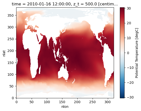
We use xarray’s isel() (select by index) function to grab the first entry in time and vertical coordinate available in our data set. Note that our dataset has some metadata associated with it, so xarray knows that the units are in degrees Celsius without us manually specifying. Xarray’s plot() function is great for looking at data quickly to make sure things look right before diving into more involved analysis or plotting.
We arbitrarily choose to plot temperature, but there are lots of options for variables to plot!
ds["TEMP"].isel(time=0, z_t=0).plot()
Making a plot on a nicer map projection
Bringing in some POP grid tools
This version of CESM uses POP2 (the Parallel Ocean Program) as its ocean model. All of the ocean variable output is on the POP grid, which requires some extra wrangling to get it to work properly with standard mapping utilities.
ds_grid = pop_tools.get_grid('POP_gx1v7')
lons = ds_grid.TLONG
lats = ds_grid.TLAT
depths = ds_grid.z_t * 0.01
In this Cookbook, we have written a function for adjusting the POP2 grid. For better code reuse, we have moved this code into a module called module.py that is imported into every notebook within this Cookbook. The content of module.py is:
display_source(adjust_pop_grid)Making the map
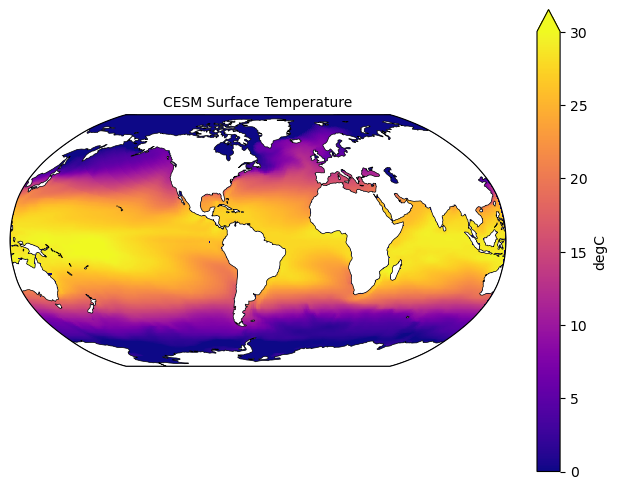
fig = plt.figure(figsize=(8,6))
ax = fig.add_subplot(1,1,1, projection=ccrs.Robinson(central_longitude=305.0))

# Using the utilities we added above to process our data, and plotting it
lon, lat, field = adjust_pop_grid(lons, lats, ds["TEMP"].isel(time=0, z_t=0))
pc1=ax.pcolormesh(lon, lat,field, cmap='plasma',
                  vmin=0, vmax=30,
                 transform=ccrs.PlateCarree())

# Adding the land features
land = cartopy.feature.NaturalEarthFeature('physical', 'land', scale='110m', edgecolor='k', facecolor='white', linewidth=0.5)
ax.add_feature(land)

# Adding colorbar and title
cbar1 = fig.colorbar(pc1, ax=ax,extend='max',label=ds["TEMP"].units)
ax.set_title('CESM Surface Temperature', fontsize=10)

plt.show()
/home/runner/micromamba/envs/ocean-bgc-cookbook-dev/lib/python3.13/site-packages/cartopy/io/__init__.py:241: DownloadWarning: Downloading: https://naturalearth.s3.amazonaws.com/110m_physical/ne_110m_land.zip
warnings.warn(f'Downloading: {url}', DownloadWarning)

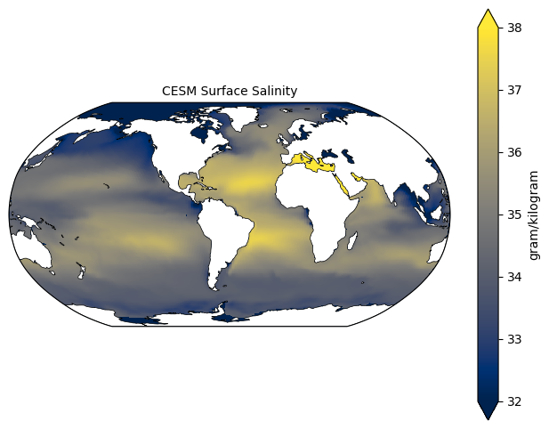
Let’s try the same thing with another variable, salinity (SALT). We replace which variable we’re extracting from ds in the adjust_pop_grid() function, where we preprocess the data. If you’re trying this on your own, some other good ones to try looking at are dissolved inorganic carbon (DIC), oxygen (O2), or pH (PH).
fig = plt.figure(figsize=(8,6))
ax = fig.add_subplot(1,1,1, projection=ccrs.Robinson(central_longitude=305.0))

# Using the utilities we added above to process our data, and plotting it
lon, lat, field = adjust_pop_grid(lons, lats, ds['SALT'].isel(time=0, z_t=0))

# Pick a different colorscheme from the plot above so we can distinguish them more easily
pc1=ax.pcolormesh(lon, lat,field, cmap='cividis',
                  vmin=32, vmax=38,
                 transform=ccrs.PlateCarree())

# Adding the land features
land = cartopy.feature.NaturalEarthFeature('physical', 'land', scale='110m', edgecolor='k', facecolor='white', linewidth=0.5)
ax.add_feature(land)

# Adding colorbar and title
cbar1 = fig.colorbar(pc1, ax=ax,extend='both',label=ds["SALT"].units)
ax.set_title('CESM Surface Salinity', fontsize=10)

plt.show()
Close the Dask cluster we spun up at the beginning.
cluster.close()Summary
You’ve learned how to make simple plots of CESM output.