Data Quality Check from the CACTI Field Campaign
Overview
Within this notebook, we will cover:
How to access multiple datasets from the Atmospheric Radiation Measurment (ARM) user facility
How to create a multipanel plot
How to compare uncorrected vs. corrected data
Prerequisites
| Concepts | Importance | Notes |
|---|---|---|
| Matplotlib Basics | Required | Basic plotting |
| Introduction to Cartopy | Helpful | Adding projections to your plot |
| Py-ART Basics | Required | IO/Visualization |
| Py-ART Corrections | Required | Radar Corrections |
Imports
import os

import act
import matplotlib as mpl
import matplotlib.pyplot as plt
import numpy as np
import cartopy.crs as ccrs
import pyart
import glob
## You are using the Python ARM Radar Toolkit (Py-ART), an open source
## library for working with weather radar data. Py-ART is partly
## supported by the U.S. Department of Energy as part of the Atmospheric
## Radiation Measurement (ARM) Climate Research Facility, an Office of
## Science user facility.
##
## If you use this software to prepare a publication, please cite:
##
##     JJ Helmus and SM Collis, JORS 2016, doi: 10.5334/jors.119
Grab Data from the ARM Data Portal
One of the better cases of the CACTI field campaign was from November 11, 2018, where several intense storms traversed through the domain.
The Cloud, Aerosol, and Complex Terrain Interactions (CACTI) Field Campaign
Data is available from the Atmospheric Radiation Measurment user facility, which helped to lead the CACTI field campaign in the Sierras de Cordoba region of Argentina.
The data are available from the ARM data portal (https://
We are interested in the corrected C-band radar data, which has the original and corrected data, with the datastream name
corcsapr2cmacppiM1.c1
Use the ARM Live API to Download the Data, using ACT
The Atmospheric Data Community Toolkit (ACT) has a helpful module to interface with the data server:
Setup our Download Query
Before downloading our data, we need to make sure we have an ARM Data Account, and ARM Live token. Both of these can be found using this link:
Once you sign up, you will see your token. Copy and replace that where we have arm_username and arm_password below.
arm_username = os.getenv("ARM_USERNAME")
arm_password = os.getenv("ARM_PASSWORD")

datastream = "corcsapr2cmacppiM1.c1"

start_date = "2018-11-11T03:00:00"
end_date = "2018-11-11T03:15:00"
csapr_files = act.discovery.download_arm_data(arm_username,
arm_password,
datastream,
start_date,
end_date,
)[DOWNLOADING] corcsapr2cmacppiM1.c1.20181111.030003.nc
If you use these data to prepare a publication, please cite:

Collis, S. C-SAPR2 Corrected Moments in Antenna Coordinates (CSAPR2CMACPPI),
2018-11-11 to 2018-11-11, ARM Mobile Facility (COR), Cordoba, Argentina; AMF1
(main site for CACTI) (M1). Atmospheric Radiation Measurement (ARM) User
Facility. https://doi.org/10.5439/1668872
Read in and Investigate our Radar Data
radar = pyart.io.read(csapr_files[0])List the available fields and plot the corrected and uncorrected data
sorted(list(radar.fields))['attenuation_corrected_differential_reflectivity',
'attenuation_corrected_differential_reflectivity_lag_1',
'attenuation_corrected_reflectivity_h',
'censor_mask',
'classification_mask',
'clutter_masked_velocity',
'copol_correlation_coeff',
'corrected_differential_phase',
'corrected_differential_reflectivity',
'corrected_reflectivity',
'corrected_specific_diff_phase',
'corrected_velocity',
'cumulative_beam_blockage',
'differential_phase',
'differential_reflectivity',
'differential_reflectivity_lag_1',
'filtered_corrected_differential_phase',
'filtered_corrected_specific_diff_phase',
'gate_id',
'ground_clutter',
'height',
'height_over_iso0',
'mean_doppler_velocity',
'mean_doppler_velocity_v',
'normalized_coherent_power',
'normalized_coherent_power_v',
'partial_beam_blockage',
'path_integrated_attenuation',
'path_integrated_differential_attenuation',
'rain_rate_A',
'reflectivity',
'reflectivity_v',
'signal_to_noise_ratio',
'signal_to_noise_ratio_copolar_h',
'signal_to_noise_ratio_copolar_v',
'simulated_velocity',
'sounding_temperature',
'specific_attenuation',
'specific_differential_attenuation',
'specific_differential_phase',
'spectral_width',
'spectral_width_v',
'uncorrected_copol_correlation_coeff',
'uncorrected_differential_phase',
'uncorrected_differential_reflectivity',
'uncorrected_differential_reflectivity_lag_1',
'uncorrected_mean_doppler_velocity_h',
'uncorrected_mean_doppler_velocity_v',
'uncorrected_reflectivity_h',
'uncorrected_reflectivity_v',
'uncorrected_spectral_width_h',
'uncorrected_spectral_width_v',
'unfolded_differential_phase',
'unthresholded_power_copolar_h',
'unthresholded_power_copolar_v',
'velocity_texture']Plot a Quick-Look of Reflectivity and Velocity
Let’s start by plotting our reflectivity and velocity fields, using a four panel plot showing the uncorrected and corrected fields. Notice how the data is masked, and the radial velocities are unfolded.
fig = plt.figure(figsize=(12,10))
display = pyart.graph.RadarDisplay(radar)
ax1 = plt.subplot(221)
display.plot_ppi("reflectivity", ax=ax1)

ax2 = plt.subplot(222)
display.plot_ppi("corrected_reflectivity", ax=ax2)

ax3 = plt.subplot(223)
display.plot_ppi("mean_doppler_velocity", vmin=-30, vmax=30, cmap='balance', ax=ax3)

ax4 = plt.subplot(224)
display.plot_ppi("corrected_velocity", vmin=-30, vmax=30, cmap='balance', ax=ax4)

plt.tight_layout()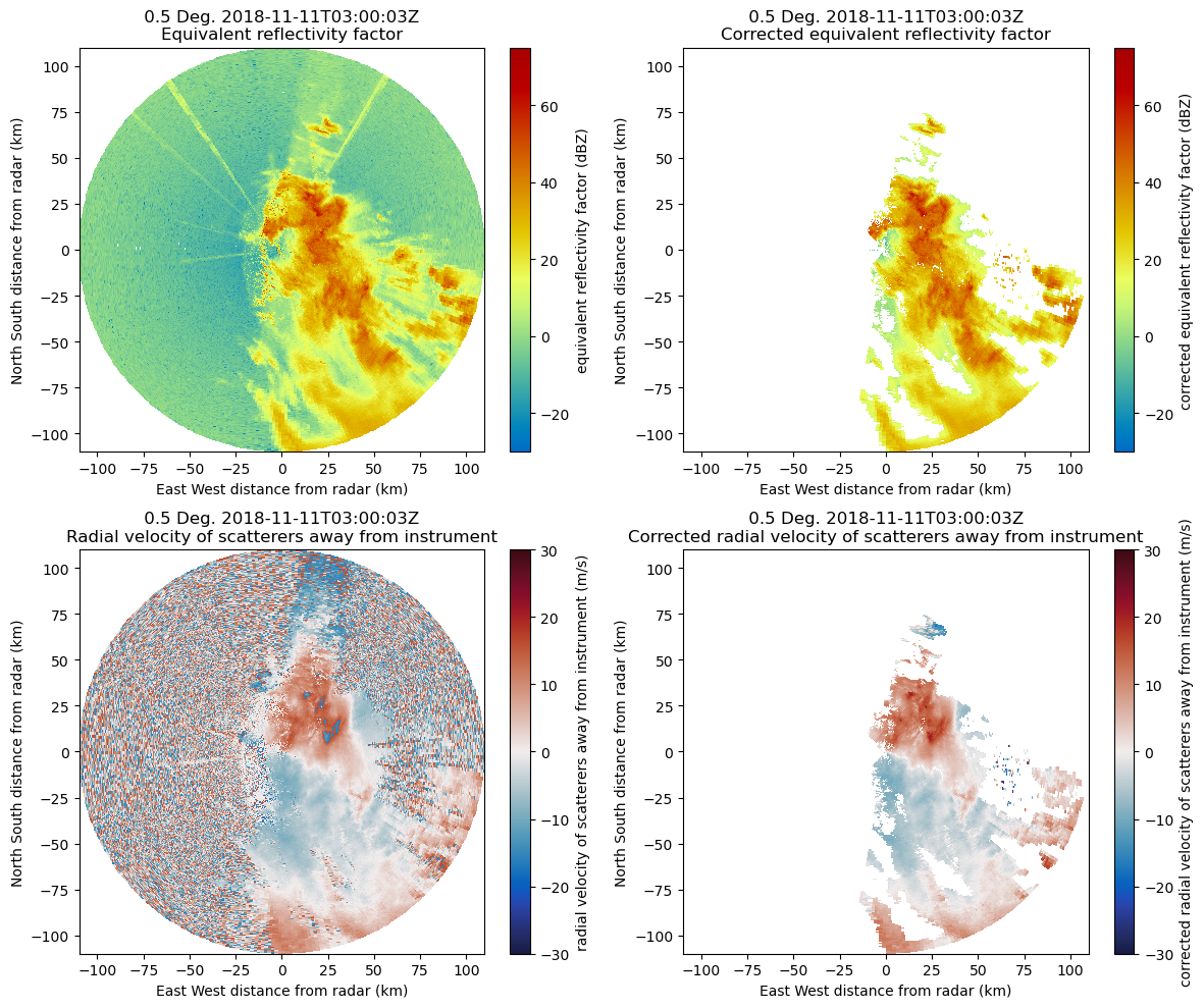
Investigate Dual-Pol Variables
Several of the variables in this file are dual-polarization products, meaning it uses pulses in both the horizontal and vertical direction, and derives fields from this additional information.
Differential Phase Shift (PhiDP) and Specific Differential Phase (KDP)
One of these dual-pol variables is called the Differential Phase Shift (PhiDP), which is the difference in 2-way attenuation for the horizontal and vertical radar pulses moving through some target. This gives us information about the shape and concentration of the features we are interested in! It is also used to calculate the specific differential phase (KDP), which is the gradient in PhiDP, where positive KDP values indicate greater phase shift in the horizontal. Higher values of KDP can indicate an increase in the size and concentration of rain drops.
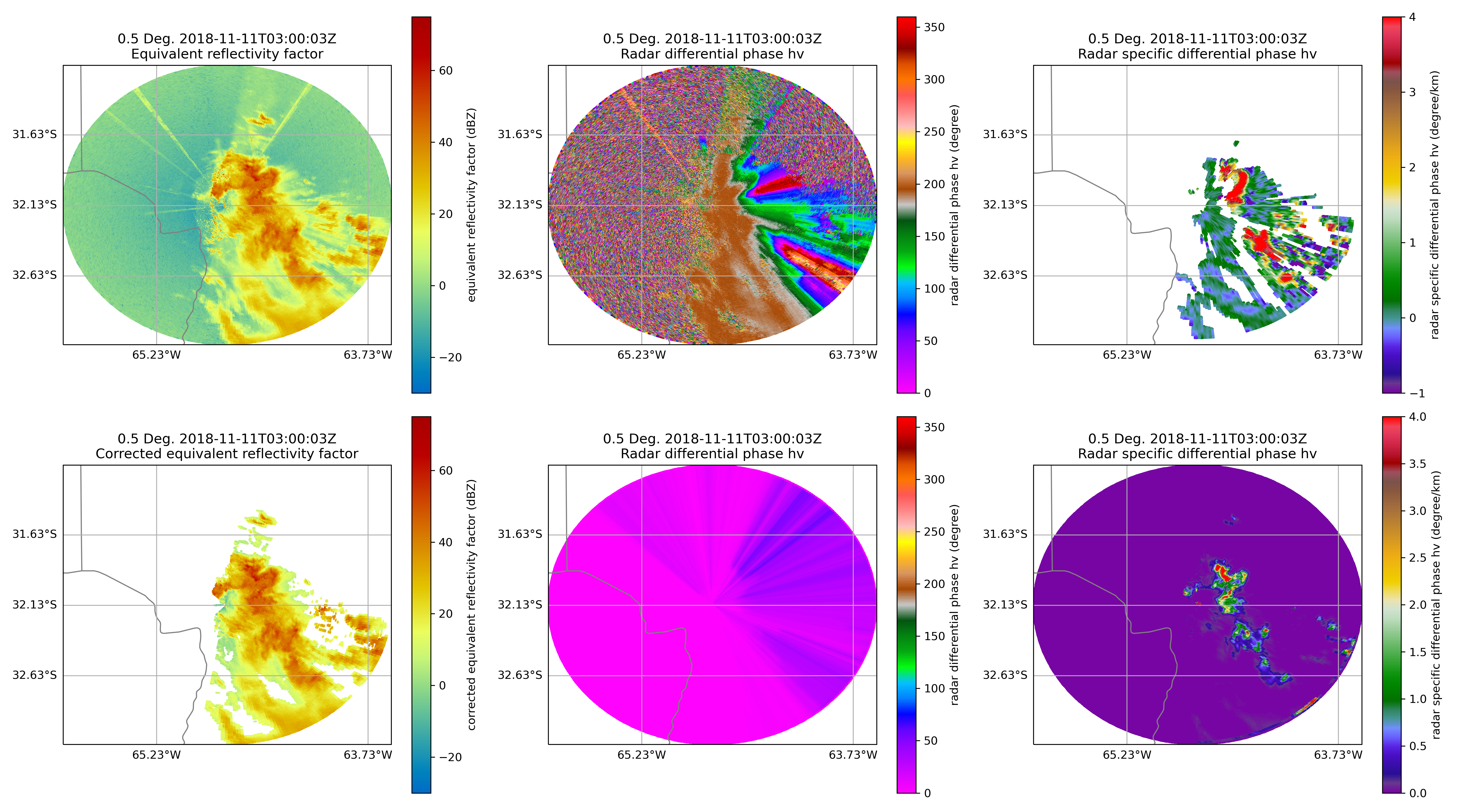
Compare Uncorrected and Corrected PhiDP and KDP
We start with the uncorrected fields, specific_differential_phase and uncorrected_differential_phase, and compare to the corrected fields filtered_corrected_specific_diff_phase and filtered_corrected_differential_phase.
Notice how much cleaner the corrected fields are, and how the noise has been filtered, leading a more analysis-ready dataset.
display = pyart.graph.RadarMapDisplay(radar)
fig = plt.figure(figsize=(18,10))

# Extract the latitude and longitude of the radar and use it for the center of the map
lat_center = round(radar.latitude['data'][0], 2)
lon_center = round(radar.longitude['data'][0], 2)

# Set the projection - in this case, we use a general PlateCarree projection
projection = ccrs.PlateCarree()

# Determine the ticks
lat_ticks = np.arange(lat_center-2, lat_center+2, .5)
lon_ticks = np.arange(lon_center-2, lon_center+2, 1.5)

ax1 = plt.subplot(231, projection=projection)
display.plot_ppi_map("reflectivity", 0, resolution='10m', ax=ax1, lat_lines=lat_ticks, lon_lines=lon_ticks)


ax3 = plt.subplot(232,projection=projection)
display.plot_ppi_map("differential_phase", 0, resolution='10m', ax=ax3, vmin=0, vmax=360, lat_lines=lat_ticks, lon_lines=lon_ticks)

ax3 = plt.subplot(233,projection=projection)
display.plot_ppi_map("specific_differential_phase", 0, resolution='10m', ax=ax3, vmin=-1, vmax=4, cmap='Carbone42', lat_lines=lat_ticks, lon_lines=lon_ticks)

ax4 = plt.subplot(234, projection=projection)
display.plot_ppi_map("corrected_reflectivity", 0, resolution='10m', ax=ax4, lat_lines=lat_ticks, lon_lines=lon_ticks)


ax5 = plt.subplot(235, projection=projection)
display.plot_ppi_map("filtered_corrected_differential_phase", 0, resolution='10m', ax=ax5, vmin=0, vmax=360, cmap='Wild25', lat_lines=lat_ticks, lon_lines=lon_ticks)

ax6 = plt.subplot(236,projection=projection)
display.plot_ppi_map("filtered_corrected_specific_diff_phase", 0, resolution='10m', ax=ax6, vmin=0, vmax=4, cmap='Carbone42', lat_lines=lat_ticks, lon_lines=lon_ticks)

plt.tight_layout()
plt.savefig('phidp_kdp_comparison_cacti.png', dpi=300, transparent=False)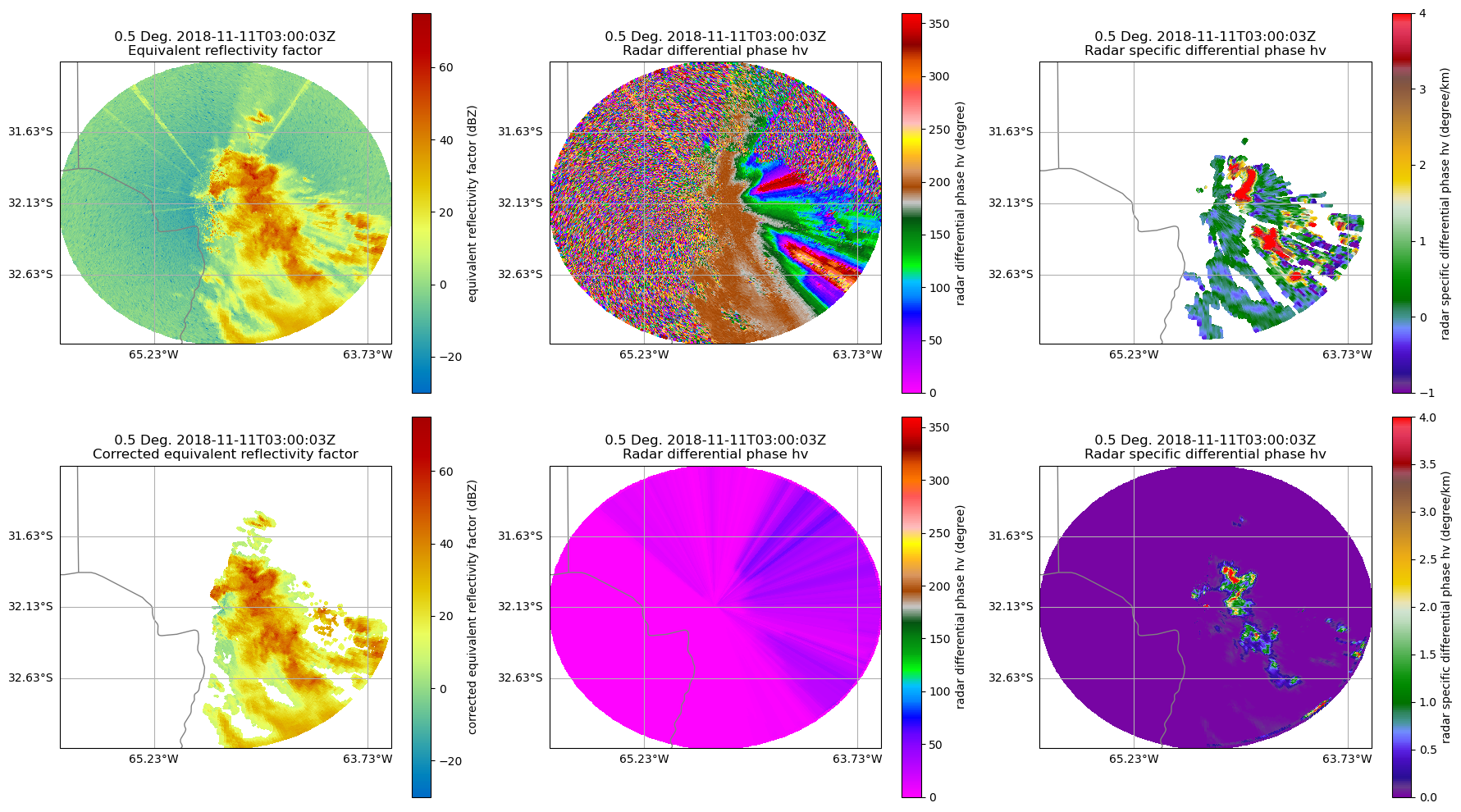
Create a Three Panel Figure Visualizing Reflectivity, Gate ID, and KDP
Now that we understand how valuable these corrections can be, let’s create a summary figure, giving a quick overview of the scatterers and associated polarimetric fields.
display = pyart.graph.RadarMapDisplay(radar)
fig = plt.figure(figsize=(18,5))

# Extract the latitude and longitude of the radar and use it for the center of the map
lat_center = round(radar.latitude['data'][0], 2)
lon_center = round(radar.longitude['data'][0], 2)

projection = ccrs.PlateCarree()

# Determine the ticks
lat_ticks = np.arange(lat_center-2, lat_center+2, .5)
lon_ticks = np.arange(lon_center-2, lon_center+2, .5)

ax1 = plt.subplot(131, projection=projection)
display.plot_ppi_map("corrected_reflectivity", 0, resolution='10m', ax=ax1, lat_lines=lat_ticks, lon_lines=lon_ticks)


ax2 = plt.subplot(132, projection=projection)
gate_ids = radar.fields["gate_id"]["flag_meanings"].split(" ")
ticks = np.arange(len(gate_ids))
boundaries = np.arange(-0.5, len(gate_ids))
norm = mpl.colors.BoundaryNorm(boundaries, 256)
display.plot_ppi_map("gate_id", 0, ax=ax2, lat_lines=lat_ticks, resolution='10m', lon_lines=lon_ticks, cmap='LangRainbow12', ticks=ticks, norm=norm, ticklabs=gate_ids)

ax3 = plt.subplot(133,projection=projection)
display.plot_ppi_map("filtered_corrected_specific_diff_phase", 0, resolution='10m', ax=ax3, vmin=0, vmax=4, cmap='Carbone42', lat_lines=lat_ticks, lon_lines=lon_ticks)

plt.tight_layout()
plt.savefig('three_panel_summary_cacti.png', dpi=300, transparent=False)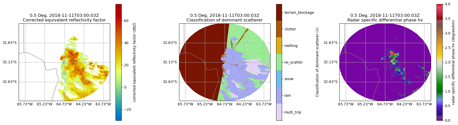
Summary
Within this example, we walked through how to access ARM data from a field campaign in Argentina, plot a quick look of the data, and compare corrected and uncorrected dual-pol variables!
What’s Next?
We will showcase other data workflow examples, including field campaigns in other regions and data access methods from other data centers.
Resources and References
CSAPR Radar Data:
Bharadwaj, N., Collis, S., Hardin, J., Isom, B., Lindenmaier, I., Matthews, A., & Nelson, D. C-Band Scanning ARM Precipitation Radar (CSAPR2CFR). Atmospheric Radiation Measurement (ARM) User Facility. Bharadwaj et al. (2021)
Py-ART:
Helmus, J.J. & Collis, S.M., (2016). The Python ARM Radar Toolkit (Py-ART), a Library for Working with Weather Radar Data in the Python Programming Language. Journal of Open Research Software. 4(1), p.e25. DOI: Helmus & Collis (2016)
ACT:
Adam Theisen, Ken Kehoe, Zach Sherman, Bobby Jackson, Alyssa Sockol, Corey Godine, Max Grover, Jason Hemedinger, Jenni Kyrouac, Maxwell Levin, Michael Giansiracusa (2022). The Atmospheric Data Community Toolkit (ACT). Zenodo. DOI: Theisen et al. (2022)
- Bharadwaj, N., Collis, S., Hardin, J., Isom, B., Lindenmaier, I., Matthews, A., Nelson, D., Feng, Y.-C., Rocque, M., Wendler, T., & Castro, V. (2021). C-Band Scanning ARM Precipitation Radar, 2nd Generation. Atmospheric Radiation Measurement (ARM) Archive, Oak Ridge National Laboratory (ORNL), Oak Ridge, TN (US); ARM Data Center, Oak Ridge National Laboratory (ORNL), Oak Ridge, TN (United States). 10.5439/1467901
- Helmus, J. J., & Collis, S. M. (2016). The Python ARM Radar Toolkit (Py-ART), a Library for Working with Weather Radar Data in the Python Programming Language. Journal of Open Research Software, 4(1), 25. 10.5334/jors.119
- Theisen, A., Kehoe, K., Sherman, Z., Jackson, B., Sockol, A., Godine, C., Grover, M., Hemedinger, J., Kyrouac, J., Levin, M., & Giansiracusa, M. (2022). ARM-DOE/ACT: ACT Release v1.1.9. Zenodo. 10.5281/ZENODO.6712343