Overview
This notebook details the steps required to perform a radiative kernel analysis.
Prerequisites
| Concepts | Importance | Notes |
|---|---|---|
| Loading CMIP6 data with Intake-ESM | Helpful | |
| Intro to Xarray | Necessary |
Time to learn: 60 minutes
Imports
import xarray as xr
import numpy as np
import matplotlib.pyplot as plt
from matplotlib.colors import CenteredNorm
import cartopy.crs as ccrs
import xesmf as xe
import intake
import s3fs
import fsspec
import globLoading in required data
Climate model output
In this example, we will perform the analysis on a single model from the CMIP6 ensemble, CESM2. The simplest way to calculate feedbacks is to take differences between two climate states, as opposed to regressions. Here we use runs with:
preindustrial conditions (
piControl) as the control climateinstantaneously quadrupled CO (
abrupt-4xCO2) as the perturbed climate
We will use CMIP6 data hosted on Pangeo’s Google Cloud Storage:
cat_url = 'https://storage.googleapis.com/cmip6/pangeo-cmip6.json'
col = intake.open_esm_datastore(cat_url)The fields (and CMIP names) required to calculate each feedback are:
Albedo: upwelling and downwelling SW radiation at the surface (
rsusandrsds)Temperature (Planck and lapse rate): air temperature (
ta) and surface temperature (ts)Water vapor: specific humidity (
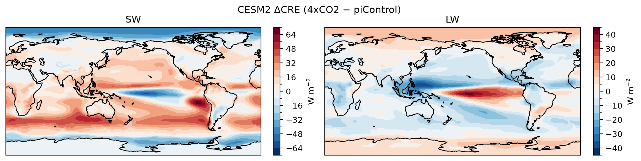
hus) and air temperatureSW CRE: Net SW radiation at TOA (down
rsdtminus uprsut) and clear-sky versions (down, which is the same, minus uprsutcs)LW CRE: Net LW radiation at TOA (
rlut) and the clear-sky version (rlutcs)
The cloud feedbacks require the results from the other feedbacks to correct for noncloud contributions to the CREs.
We will also need near-surface air temperature (tas) for calculating the change in global mean surface temperature (GMST).
cat = col.search(activity_id='CMIP', experiment_id=['piControl', 'abrupt-4xCO2'], table_id='Amon', source_id='CESM2',
variable_id=['rsus', 'rsds', 'ta', 'ts', 'hus', 'rsdt', 'rsut', 'rsutcs', 'rlut', 'rlutcs', 'tas'])
cat.dfdset_dict = cat.to_dataset_dict(zarr_kwargs={'consolidated': True})
--> The keys in the returned dictionary of datasets are constructed as follows:
'activity_id.institution_id.source_id.experiment_id.table_id.grid_label'
Could not determine bucket type for bucket name cmip6: Your default credentials were not found. To set up Application Default Credentials, see https://cloud.google.com/docs/authentication/external/set-up-adc for more information., falling back to GCSFileSystem
Could not determine bucket type for bucket name cmip6: Your default credentials were not found. To set up Application Default Credentials, see https://cloud.google.com/docs/authentication/external/set-up-adc for more information., falling back to GCSFileSystem
Could not determine bucket type for bucket name cmip6: Your default credentials were not found. To set up Application Default Credentials, see https://cloud.google.com/docs/authentication/external/set-up-adc for more information., falling back to GCSFileSystem
Could not determine bucket type for bucket name cmip6: Your default credentials were not found. To set up Application Default Credentials, see https://cloud.google.com/docs/authentication/external/set-up-adc for more information., falling back to GCSFileSystem
Could not determine bucket type for bucket name cmip6: Your default credentials were not found. To set up Application Default Credentials, see https://cloud.google.com/docs/authentication/external/set-up-adc for more information., falling back to GCSFileSystem
Could not determine bucket type for bucket name cmip6: Your default credentials were not found. To set up Application Default Credentials, see https://cloud.google.com/docs/authentication/external/set-up-adc for more information., falling back to GCSFileSystem
Could not determine bucket type for bucket name cmip6: Your default credentials were not found. To set up Application Default Credentials, see https://cloud.google.com/docs/authentication/external/set-up-adc for more information., falling back to GCSFileSystem
Could not determine bucket type for bucket name cmip6: Your default credentials were not found. To set up Application Default Credentials, see https://cloud.google.com/docs/authentication/external/set-up-adc for more information., falling back to GCSFileSystem
Could not determine bucket type for bucket name cmip6: Your default credentials were not found. To set up Application Default Credentials, see https://cloud.google.com/docs/authentication/external/set-up-adc for more information., falling back to GCSFileSystem
Could not determine bucket type for bucket name cmip6: Your default credentials were not found. To set up Application Default Credentials, see https://cloud.google.com/docs/authentication/external/set-up-adc for more information., falling back to GCSFileSystem
Could not determine bucket type for bucket name cmip6: Your default credentials were not found. To set up Application Default Credentials, see https://cloud.google.com/docs/authentication/external/set-up-adc for more information., falling back to GCSFileSystem
Could not determine bucket type for bucket name cmip6: Your default credentials were not found. To set up Application Default Credentials, see https://cloud.google.com/docs/authentication/external/set-up-adc for more information., falling back to GCSFileSystem
Could not determine bucket type for bucket name cmip6: Your default credentials were not found. To set up Application Default Credentials, see https://cloud.google.com/docs/authentication/external/set-up-adc for more information., falling back to GCSFileSystem
Could not determine bucket type for bucket name cmip6: Your default credentials were not found. To set up Application Default Credentials, see https://cloud.google.com/docs/authentication/external/set-up-adc for more information., falling back to GCSFileSystem
Could not determine bucket type for bucket name cmip6: Your default credentials were not found. To set up Application Default Credentials, see https://cloud.google.com/docs/authentication/external/set-up-adc for more information., falling back to GCSFileSystem
Could not determine bucket type for bucket name cmip6: Your default credentials were not found. To set up Application Default Credentials, see https://cloud.google.com/docs/authentication/external/set-up-adc for more information., falling back to GCSFileSystem
Could not determine bucket type for bucket name cmip6: Your default credentials were not found. To set up Application Default Credentials, see https://cloud.google.com/docs/authentication/external/set-up-adc for more information., falling back to GCSFileSystem
Could not determine bucket type for bucket name cmip6: Your default credentials were not found. To set up Application Default Credentials, see https://cloud.google.com/docs/authentication/external/set-up-adc for more information., falling back to GCSFileSystem
Could not determine bucket type for bucket name cmip6: Your default credentials were not found. To set up Application Default Credentials, see https://cloud.google.com/docs/authentication/external/set-up-adc for more information., falling back to GCSFileSystem
Could not determine bucket type for bucket name cmip6: Your default credentials were not found. To set up Application Default Credentials, see https://cloud.google.com/docs/authentication/external/set-up-adc for more information., falling back to GCSFileSystem
Could not determine bucket type for bucket name cmip6: Your default credentials were not found. To set up Application Default Credentials, see https://cloud.google.com/docs/authentication/external/set-up-adc for more information., falling back to GCSFileSystem
Could not determine bucket type for bucket name cmip6: Your default credentials were not found. To set up Application Default Credentials, see https://cloud.google.com/docs/authentication/external/set-up-adc for more information., falling back to GCSFileSystem
Could not determine bucket type for bucket name cmip6: Your default credentials were not found. To set up Application Default Credentials, see https://cloud.google.com/docs/authentication/external/set-up-adc for more information., falling back to GCSFileSystem
Could not determine bucket type for bucket name cmip6: Your default credentials were not found. To set up Application Default Credentials, see https://cloud.google.com/docs/authentication/external/set-up-adc for more information., falling back to GCSFileSystem
Could not determine bucket type for bucket name cmip6: Your default credentials were not found. To set up Application Default Credentials, see https://cloud.google.com/docs/authentication/external/set-up-adc for more information., falling back to GCSFileSystem
Could not determine bucket type for bucket name cmip6: Your default credentials were not found. To set up Application Default Credentials, see https://cloud.google.com/docs/authentication/external/set-up-adc for more information., falling back to GCSFileSystem
Could not determine bucket type for bucket name cmip6: Your default credentials were not found. To set up Application Default Credentials, see https://cloud.google.com/docs/authentication/external/set-up-adc for more information., falling back to GCSFileSystem
Could not determine bucket type for bucket name cmip6: Your default credentials were not found. To set up Application Default Credentials, see https://cloud.google.com/docs/authentication/external/set-up-adc for more information., falling back to GCSFileSystem
Could not determine bucket type for bucket name cmip6: Your default credentials were not found. To set up Application Default Credentials, see https://cloud.google.com/docs/authentication/external/set-up-adc for more information., falling back to GCSFileSystem
Could not determine bucket type for bucket name cmip6: Your default credentials were not found. To set up Application Default Credentials, see https://cloud.google.com/docs/authentication/external/set-up-adc for more information., falling back to GCSFileSystem
Could not determine bucket type for bucket name cmip6: Your default credentials were not found. To set up Application Default Credentials, see https://cloud.google.com/docs/authentication/external/set-up-adc for more information., falling back to GCSFileSystem
Could not determine bucket type for bucket name cmip6: Your default credentials were not found. To set up Application Default Credentials, see https://cloud.google.com/docs/authentication/external/set-up-adc for more information., falling back to GCSFileSystem
Could not determine bucket type for bucket name cmip6: Your default credentials were not found. To set up Application Default Credentials, see https://cloud.google.com/docs/authentication/external/set-up-adc for more information., falling back to GCSFileSystem
Could not determine bucket type for bucket name cmip6: Your default credentials were not found. To set up Application Default Credentials, see https://cloud.google.com/docs/authentication/external/set-up-adc for more information., falling back to GCSFileSystem
Could not determine bucket type for bucket name cmip6: Your default credentials were not found. To set up Application Default Credentials, see https://cloud.google.com/docs/authentication/external/set-up-adc for more information., falling back to GCSFileSystem
Could not determine bucket type for bucket name cmip6: Your default credentials were not found. To set up Application Default Credentials, see https://cloud.google.com/docs/authentication/external/set-up-adc for more information., falling back to GCSFileSystem
Could not determine bucket type for bucket name cmip6: Your default credentials were not found. To set up Application Default Credentials, see https://cloud.google.com/docs/authentication/external/set-up-adc for more information., falling back to GCSFileSystem
Could not determine bucket type for bucket name cmip6: Your default credentials were not found. To set up Application Default Credentials, see https://cloud.google.com/docs/authentication/external/set-up-adc for more information., falling back to GCSFileSystem
Could not determine bucket type for bucket name cmip6: Your default credentials were not found. To set up Application Default Credentials, see https://cloud.google.com/docs/authentication/external/set-up-adc for more information., falling back to GCSFileSystem
Could not determine bucket type for bucket name cmip6: Your default credentials were not found. To set up Application Default Credentials, see https://cloud.google.com/docs/authentication/external/set-up-adc for more information., falling back to GCSFileSystem
Could not determine bucket type for bucket name cmip6: Your default credentials were not found. To set up Application Default Credentials, see https://cloud.google.com/docs/authentication/external/set-up-adc for more information., falling back to GCSFileSystem
Could not determine bucket type for bucket name cmip6: Your default credentials were not found. To set up Application Default Credentials, see https://cloud.google.com/docs/authentication/external/set-up-adc for more information., falling back to GCSFileSystem
Could not determine bucket type for bucket name cmip6: Your default credentials were not found. To set up Application Default Credentials, see https://cloud.google.com/docs/authentication/external/set-up-adc for more information., falling back to GCSFileSystem
Could not determine bucket type for bucket name cmip6: Your default credentials were not found. To set up Application Default Credentials, see https://cloud.google.com/docs/authentication/external/set-up-adc for more information., falling back to GCSFileSystem
Could not determine bucket type for bucket name cmip6: Your default credentials were not found. To set up Application Default Credentials, see https://cloud.google.com/docs/authentication/external/set-up-adc for more information., falling back to GCSFileSystem
Could not determine bucket type for bucket name cmip6: Your default credentials were not found. To set up Application Default Credentials, see https://cloud.google.com/docs/authentication/external/set-up-adc for more information., falling back to GCSFileSystem
Could not determine bucket type for bucket name cmip6: Your default credentials were not found. To set up Application Default Credentials, see https://cloud.google.com/docs/authentication/external/set-up-adc for more information., falling back to GCSFileSystem
Could not determine bucket type for bucket name cmip6: Your default credentials were not found. To set up Application Default Credentials, see https://cloud.google.com/docs/authentication/external/set-up-adc for more information., falling back to GCSFileSystem
Could not determine bucket type for bucket name cmip6: Your default credentials were not found. To set up Application Default Credentials, see https://cloud.google.com/docs/authentication/external/set-up-adc for more information., falling back to GCSFileSystem
Could not determine bucket type for bucket name cmip6: Your default credentials were not found. To set up Application Default Credentials, see https://cloud.google.com/docs/authentication/external/set-up-adc for more information., falling back to GCSFileSystem
Could not determine bucket type for bucket name cmip6: Your default credentials were not found. To set up Application Default Credentials, see https://cloud.google.com/docs/authentication/external/set-up-adc for more information., falling back to GCSFileSystem
Could not determine bucket type for bucket name cmip6: Your default credentials were not found. To set up Application Default Credentials, see https://cloud.google.com/docs/authentication/external/set-up-adc for more information., falling back to GCSFileSystem
Could not determine bucket type for bucket name cmip6: Your default credentials were not found. To set up Application Default Credentials, see https://cloud.google.com/docs/authentication/external/set-up-adc for more information., falling back to GCSFileSystem
Could not determine bucket type for bucket name cmip6: Your default credentials were not found. To set up Application Default Credentials, see https://cloud.google.com/docs/authentication/external/set-up-adc for more information., falling back to GCSFileSystem
Could not determine bucket type for bucket name cmip6: Your default credentials were not found. To set up Application Default Credentials, see https://cloud.google.com/docs/authentication/external/set-up-adc for more information., falling back to GCSFileSystem
Could not determine bucket type for bucket name cmip6: Your default credentials were not found. To set up Application Default Credentials, see https://cloud.google.com/docs/authentication/external/set-up-adc for more information., falling back to GCSFileSystem
Could not determine bucket type for bucket name cmip6: Your default credentials were not found. To set up Application Default Credentials, see https://cloud.google.com/docs/authentication/external/set-up-adc for more information., falling back to GCSFileSystem
Could not determine bucket type for bucket name cmip6: Your default credentials were not found. To set up Application Default Credentials, see https://cloud.google.com/docs/authentication/external/set-up-adc for more information., falling back to GCSFileSystem
Could not determine bucket type for bucket name cmip6: Your default credentials were not found. To set up Application Default Credentials, see https://cloud.google.com/docs/authentication/external/set-up-adc for more information., falling back to GCSFileSystem
Could not determine bucket type for bucket name cmip6: Your default credentials were not found. To set up Application Default Credentials, see https://cloud.google.com/docs/authentication/external/set-up-adc for more information., falling back to GCSFileSystem
Could not determine bucket type for bucket name cmip6: Your default credentials were not found. To set up Application Default Credentials, see https://cloud.google.com/docs/authentication/external/set-up-adc for more information., falling back to GCSFileSystem
Could not determine bucket type for bucket name cmip6: Your default credentials were not found. To set up Application Default Credentials, see https://cloud.google.com/docs/authentication/external/set-up-adc for more information., falling back to GCSFileSystem
Could not determine bucket type for bucket name cmip6: Your default credentials were not found. To set up Application Default Credentials, see https://cloud.google.com/docs/authentication/external/set-up-adc for more information., falling back to GCSFileSystem
Could not determine bucket type for bucket name cmip6: Your default credentials were not found. To set up Application Default Credentials, see https://cloud.google.com/docs/authentication/external/set-up-adc for more information., falling back to GCSFileSystem
Could not determine bucket type for bucket name cmip6: Your default credentials were not found. To set up Application Default Credentials, see https://cloud.google.com/docs/authentication/external/set-up-adc for more information., falling back to GCSFileSystem
Could not determine bucket type for bucket name cmip6: Your default credentials were not found. To set up Application Default Credentials, see https://cloud.google.com/docs/authentication/external/set-up-adc for more information., falling back to GCSFileSystem
Could not determine bucket type for bucket name cmip6: Your default credentials were not found. To set up Application Default Credentials, see https://cloud.google.com/docs/authentication/external/set-up-adc for more information., falling back to GCSFileSystem
Could not determine bucket type for bucket name cmip6: Your default credentials were not found. To set up Application Default Credentials, see https://cloud.google.com/docs/authentication/external/set-up-adc for more information., falling back to GCSFileSystem
Could not determine bucket type for bucket name cmip6: Your default credentials were not found. To set up Application Default Credentials, see https://cloud.google.com/docs/authentication/external/set-up-adc for more information., falling back to GCSFileSystem
Could not determine bucket type for bucket name cmip6: Your default credentials were not found. To set up Application Default Credentials, see https://cloud.google.com/docs/authentication/external/set-up-adc for more information., falling back to GCSFileSystem
Could not determine bucket type for bucket name cmip6: Your default credentials were not found. To set up Application Default Credentials, see https://cloud.google.com/docs/authentication/external/set-up-adc for more information., falling back to GCSFileSystem
Could not determine bucket type for bucket name cmip6: Your default credentials were not found. To set up Application Default Credentials, see https://cloud.google.com/docs/authentication/external/set-up-adc for more information., falling back to GCSFileSystem
Could not determine bucket type for bucket name cmip6: Your default credentials were not found. To set up Application Default Credentials, see https://cloud.google.com/docs/authentication/external/set-up-adc for more information., falling back to GCSFileSystem
Could not determine bucket type for bucket name cmip6: Your default credentials were not found. To set up Application Default Credentials, see https://cloud.google.com/docs/authentication/external/set-up-adc for more information., falling back to GCSFileSystem
Could not determine bucket type for bucket name cmip6: Your default credentials were not found. To set up Application Default Credentials, see https://cloud.google.com/docs/authentication/external/set-up-adc for more information., falling back to GCSFileSystem
Could not determine bucket type for bucket name cmip6: Your default credentials were not found. To set up Application Default Credentials, see https://cloud.google.com/docs/authentication/external/set-up-adc for more information., falling back to GCSFileSystem
Could not determine bucket type for bucket name cmip6: Your default credentials were not found. To set up Application Default Credentials, see https://cloud.google.com/docs/authentication/external/set-up-adc for more information., falling back to GCSFileSystem
Could not determine bucket type for bucket name cmip6: Your default credentials were not found. To set up Application Default Credentials, see https://cloud.google.com/docs/authentication/external/set-up-adc for more information., falling back to GCSFileSystem
Could not determine bucket type for bucket name cmip6: Your default credentials were not found. To set up Application Default Credentials, see https://cloud.google.com/docs/authentication/external/set-up-adc for more information., falling back to GCSFileSystem
Could not determine bucket type for bucket name cmip6: Your default credentials were not found. To set up Application Default Credentials, see https://cloud.google.com/docs/authentication/external/set-up-adc for more information., falling back to GCSFileSystem
Could not determine bucket type for bucket name cmip6: Your default credentials were not found. To set up Application Default Credentials, see https://cloud.google.com/docs/authentication/external/set-up-adc for more information., falling back to GCSFileSystem
Could not determine bucket type for bucket name cmip6: Your default credentials were not found. To set up Application Default Credentials, see https://cloud.google.com/docs/authentication/external/set-up-adc for more information., falling back to GCSFileSystem
Could not determine bucket type for bucket name cmip6: Your default credentials were not found. To set up Application Default Credentials, see https://cloud.google.com/docs/authentication/external/set-up-adc for more information., falling back to GCSFileSystem
Could not determine bucket type for bucket name cmip6: Your default credentials were not found. To set up Application Default Credentials, see https://cloud.google.com/docs/authentication/external/set-up-adc for more information., falling back to GCSFileSystem
Could not determine bucket type for bucket name cmip6: Your default credentials were not found. To set up Application Default Credentials, see https://cloud.google.com/docs/authentication/external/set-up-adc for more information., falling back to GCSFileSystem
Could not determine bucket type for bucket name cmip6: Your default credentials were not found. To set up Application Default Credentials, see https://cloud.google.com/docs/authentication/external/set-up-adc for more information., falling back to GCSFileSystem
Could not determine bucket type for bucket name cmip6: Your default credentials were not found. To set up Application Default Credentials, see https://cloud.google.com/docs/authentication/external/set-up-adc for more information., falling back to GCSFileSystem
Could not determine bucket type for bucket name cmip6: Your default credentials were not found. To set up Application Default Credentials, see https://cloud.google.com/docs/authentication/external/set-up-adc for more information., falling back to GCSFileSystem
Could not determine bucket type for bucket name cmip6: Your default credentials were not found. To set up Application Default Credentials, see https://cloud.google.com/docs/authentication/external/set-up-adc for more information., falling back to GCSFileSystem
Could not determine bucket type for bucket name cmip6: Your default credentials were not found. To set up Application Default Credentials, see https://cloud.google.com/docs/authentication/external/set-up-adc for more information., falling back to GCSFileSystem
Could not determine bucket type for bucket name cmip6: Your default credentials were not found. To set up Application Default Credentials, see https://cloud.google.com/docs/authentication/external/set-up-adc for more information., falling back to GCSFileSystem
Could not determine bucket type for bucket name cmip6: Your default credentials were not found. To set up Application Default Credentials, see https://cloud.google.com/docs/authentication/external/set-up-adc for more information., falling back to GCSFileSystem
Could not determine bucket type for bucket name cmip6: Your default credentials were not found. To set up Application Default Credentials, see https://cloud.google.com/docs/authentication/external/set-up-adc for more information., falling back to GCSFileSystem
Could not determine bucket type for bucket name cmip6: Your default credentials were not found. To set up Application Default Credentials, see https://cloud.google.com/docs/authentication/external/set-up-adc for more information., falling back to GCSFileSystem
Could not determine bucket type for bucket name cmip6: Your default credentials were not found. To set up Application Default Credentials, see https://cloud.google.com/docs/authentication/external/set-up-adc for more information., falling back to GCSFileSystem
Could not determine bucket type for bucket name cmip6: Your default credentials were not found. To set up Application Default Credentials, see https://cloud.google.com/docs/authentication/external/set-up-adc for more information., falling back to GCSFileSystem
Could not determine bucket type for bucket name cmip6: Your default credentials were not found. To set up Application Default Credentials, see https://cloud.google.com/docs/authentication/external/set-up-adc for more information., falling back to GCSFileSystem
Could not determine bucket type for bucket name cmip6: Your default credentials were not found. To set up Application Default Credentials, see https://cloud.google.com/docs/authentication/external/set-up-adc for more information., falling back to GCSFileSystem
Could not determine bucket type for bucket name cmip6: Your default credentials were not found. To set up Application Default Credentials, see https://cloud.google.com/docs/authentication/external/set-up-adc for more information., falling back to GCSFileSystem
Could not determine bucket type for bucket name cmip6: Your default credentials were not found. To set up Application Default Credentials, see https://cloud.google.com/docs/authentication/external/set-up-adc for more information., falling back to GCSFileSystem
Could not determine bucket type for bucket name cmip6: Your default credentials were not found. To set up Application Default Credentials, see https://cloud.google.com/docs/authentication/external/set-up-adc for more information., falling back to GCSFileSystem
Could not determine bucket type for bucket name cmip6: Your default credentials were not found. To set up Application Default Credentials, see https://cloud.google.com/docs/authentication/external/set-up-adc for more information., falling back to GCSFileSystem
Could not determine bucket type for bucket name cmip6: Your default credentials were not found. To set up Application Default Credentials, see https://cloud.google.com/docs/authentication/external/set-up-adc for more information., falling back to GCSFileSystem
Could not determine bucket type for bucket name cmip6: Your default credentials were not found. To set up Application Default Credentials, see https://cloud.google.com/docs/authentication/external/set-up-adc for more information., falling back to GCSFileSystem
Could not determine bucket type for bucket name cmip6: Your default credentials were not found. To set up Application Default Credentials, see https://cloud.google.com/docs/authentication/external/set-up-adc for more information., falling back to GCSFileSystem
Could not determine bucket type for bucket name cmip6: Your default credentials were not found. To set up Application Default Credentials, see https://cloud.google.com/docs/authentication/external/set-up-adc for more information., falling back to GCSFileSystem
Could not determine bucket type for bucket name cmip6: Your default credentials were not found. To set up Application Default Credentials, see https://cloud.google.com/docs/authentication/external/set-up-adc for more information., falling back to GCSFileSystem
Could not determine bucket type for bucket name cmip6: Your default credentials were not found. To set up Application Default Credentials, see https://cloud.google.com/docs/authentication/external/set-up-adc for more information., falling back to GCSFileSystem
Could not determine bucket type for bucket name cmip6: Your default credentials were not found. To set up Application Default Credentials, see https://cloud.google.com/docs/authentication/external/set-up-adc for more information., falling back to GCSFileSystem
Could not determine bucket type for bucket name cmip6: Your default credentials were not found. To set up Application Default Credentials, see https://cloud.google.com/docs/authentication/external/set-up-adc for more information., falling back to GCSFileSystem
Could not determine bucket type for bucket name cmip6: Your default credentials were not found. To set up Application Default Credentials, see https://cloud.google.com/docs/authentication/external/set-up-adc for more information., falling back to GCSFileSystem
Could not determine bucket type for bucket name cmip6: Your default credentials were not found. To set up Application Default Credentials, see https://cloud.google.com/docs/authentication/external/set-up-adc for more information., falling back to GCSFileSystem
Could not determine bucket type for bucket name cmip6: Your default credentials were not found. To set up Application Default Credentials, see https://cloud.google.com/docs/authentication/external/set-up-adc for more information., falling back to GCSFileSystem
Could not determine bucket type for bucket name cmip6: Your default credentials were not found. To set up Application Default Credentials, see https://cloud.google.com/docs/authentication/external/set-up-adc for more information., falling back to GCSFileSystem
Could not determine bucket type for bucket name cmip6: Your default credentials were not found. To set up Application Default Credentials, see https://cloud.google.com/docs/authentication/external/set-up-adc for more information., falling back to GCSFileSystem
Could not determine bucket type for bucket name cmip6: Your default credentials were not found. To set up Application Default Credentials, see https://cloud.google.com/docs/authentication/external/set-up-adc for more information., falling back to GCSFileSystem
Could not determine bucket type for bucket name cmip6: Your default credentials were not found. To set up Application Default Credentials, see https://cloud.google.com/docs/authentication/external/set-up-adc for more information., falling back to GCSFileSystem
Could not determine bucket type for bucket name cmip6: Your default credentials were not found. To set up Application Default Credentials, see https://cloud.google.com/docs/authentication/external/set-up-adc for more information., falling back to GCSFileSystem
Could not determine bucket type for bucket name cmip6: Your default credentials were not found. To set up Application Default Credentials, see https://cloud.google.com/docs/authentication/external/set-up-adc for more information., falling back to GCSFileSystem
Could not determine bucket type for bucket name cmip6: Your default credentials were not found. To set up Application Default Credentials, see https://cloud.google.com/docs/authentication/external/set-up-adc for more information., falling back to GCSFileSystem
Could not determine bucket type for bucket name cmip6: Your default credentials were not found. To set up Application Default Credentials, see https://cloud.google.com/docs/authentication/external/set-up-adc for more information., falling back to GCSFileSystem
Could not determine bucket type for bucket name cmip6: Your default credentials were not found. To set up Application Default Credentials, see https://cloud.google.com/docs/authentication/external/set-up-adc for more information., falling back to GCSFileSystem
Could not determine bucket type for bucket name cmip6: Your default credentials were not found. To set up Application Default Credentials, see https://cloud.google.com/docs/authentication/external/set-up-adc for more information., falling back to GCSFileSystem
Could not determine bucket type for bucket name cmip6: Your default credentials were not found. To set up Application Default Credentials, see https://cloud.google.com/docs/authentication/external/set-up-adc for more information., falling back to GCSFileSystem
Could not determine bucket type for bucket name cmip6: Your default credentials were not found. To set up Application Default Credentials, see https://cloud.google.com/docs/authentication/external/set-up-adc for more information., falling back to GCSFileSystem
Could not determine bucket type for bucket name cmip6: Your default credentials were not found. To set up Application Default Credentials, see https://cloud.google.com/docs/authentication/external/set-up-adc for more information., falling back to GCSFileSystem
Could not determine bucket type for bucket name cmip6: Your default credentials were not found. To set up Application Default Credentials, see https://cloud.google.com/docs/authentication/external/set-up-adc for more information., falling back to GCSFileSystem
Could not determine bucket type for bucket name cmip6: Your default credentials were not found. To set up Application Default Credentials, see https://cloud.google.com/docs/authentication/external/set-up-adc for more information., falling back to GCSFileSystem
Could not determine bucket type for bucket name cmip6: Your default credentials were not found. To set up Application Default Credentials, see https://cloud.google.com/docs/authentication/external/set-up-adc for more information., falling back to GCSFileSystem
Could not determine bucket type for bucket name cmip6: Your default credentials were not found. To set up Application Default Credentials, see https://cloud.google.com/docs/authentication/external/set-up-adc for more information., falling back to GCSFileSystem
Could not determine bucket type for bucket name cmip6: Your default credentials were not found. To set up Application Default Credentials, see https://cloud.google.com/docs/authentication/external/set-up-adc for more information., falling back to GCSFileSystem
Could not determine bucket type for bucket name cmip6: Your default credentials were not found. To set up Application Default Credentials, see https://cloud.google.com/docs/authentication/external/set-up-adc for more information., falling back to GCSFileSystem
Could not determine bucket type for bucket name cmip6: Your default credentials were not found. To set up Application Default Credentials, see https://cloud.google.com/docs/authentication/external/set-up-adc for more information., falling back to GCSFileSystem
Could not determine bucket type for bucket name cmip6: Your default credentials were not found. To set up Application Default Credentials, see https://cloud.google.com/docs/authentication/external/set-up-adc for more information., falling back to GCSFileSystem
Could not determine bucket type for bucket name cmip6: Your default credentials were not found. To set up Application Default Credentials, see https://cloud.google.com/docs/authentication/external/set-up-adc for more information., falling back to GCSFileSystem
Could not determine bucket type for bucket name cmip6: Your default credentials were not found. To set up Application Default Credentials, see https://cloud.google.com/docs/authentication/external/set-up-adc for more information., falling back to GCSFileSystem
Could not determine bucket type for bucket name cmip6: Your default credentials were not found. To set up Application Default Credentials, see https://cloud.google.com/docs/authentication/external/set-up-adc for more information., falling back to GCSFileSystem
Could not determine bucket type for bucket name cmip6: Your default credentials were not found. To set up Application Default Credentials, see https://cloud.google.com/docs/authentication/external/set-up-adc for more information., falling back to GCSFileSystem
Could not determine bucket type for bucket name cmip6: Your default credentials were not found. To set up Application Default Credentials, see https://cloud.google.com/docs/authentication/external/set-up-adc for more information., falling back to GCSFileSystem
Could not determine bucket type for bucket name cmip6: Your default credentials were not found. To set up Application Default Credentials, see https://cloud.google.com/docs/authentication/external/set-up-adc for more information., falling back to GCSFileSystem
/home/runner/micromamba/envs/feedback-cookbook-dev/lib/python3.14/site-packages/intake_esm/source.py:109: UserWarning: The specified chunks separate the stored chunks along dimension "time" starting at index 650. This could degrade performance. Instead, consider rechunking after loading.
ds = xr.open_dataset(url, **xarray_open_kwargs)
/home/runner/micromamba/envs/feedback-cookbook-dev/lib/python3.14/site-packages/intake_esm/source.py:109: UserWarning: The specified chunks separate the stored chunks along dimension "lat" starting at index 185. This could degrade performance. Instead, consider rechunking after loading.
ds = xr.open_dataset(url, **xarray_open_kwargs)
/home/runner/micromamba/envs/feedback-cookbook-dev/lib/python3.14/site-packages/intake_esm/source.py:109: UserWarning: The specified chunks separate the stored chunks along dimension "lon" starting at index 278. This could degrade performance. Instead, consider rechunking after loading.
ds = xr.open_dataset(url, **xarray_open_kwargs)
Could not determine bucket type for bucket name cmip6: Your default credentials were not found. To set up Application Default Credentials, see https://cloud.google.com/docs/authentication/external/set-up-adc for more information., falling back to GCSFileSystem
Could not determine bucket type for bucket name cmip6: Your default credentials were not found. To set up Application Default Credentials, see https://cloud.google.com/docs/authentication/external/set-up-adc for more information., falling back to GCSFileSystem
Could not determine bucket type for bucket name cmip6: Your default credentials were not found. To set up Application Default Credentials, see https://cloud.google.com/docs/authentication/external/set-up-adc for more information., falling back to GCSFileSystem
Could not determine bucket type for bucket name cmip6: Your default credentials were not found. To set up Application Default Credentials, see https://cloud.google.com/docs/authentication/external/set-up-adc for more information., falling back to GCSFileSystem
Could not determine bucket type for bucket name cmip6: Your default credentials were not found. To set up Application Default Credentials, see https://cloud.google.com/docs/authentication/external/set-up-adc for more information., falling back to GCSFileSystem
Could not determine bucket type for bucket name cmip6: Your default credentials were not found. To set up Application Default Credentials, see https://cloud.google.com/docs/authentication/external/set-up-adc for more information., falling back to GCSFileSystem
Could not determine bucket type for bucket name cmip6: Your default credentials were not found. To set up Application Default Credentials, see https://cloud.google.com/docs/authentication/external/set-up-adc for more information., falling back to GCSFileSystem
Could not determine bucket type for bucket name cmip6: Your default credentials were not found. To set up Application Default Credentials, see https://cloud.google.com/docs/authentication/external/set-up-adc for more information., falling back to GCSFileSystem
Could not determine bucket type for bucket name cmip6: Your default credentials were not found. To set up Application Default Credentials, see https://cloud.google.com/docs/authentication/external/set-up-adc for more information., falling back to GCSFileSystem
Could not determine bucket type for bucket name cmip6: Your default credentials were not found. To set up Application Default Credentials, see https://cloud.google.com/docs/authentication/external/set-up-adc for more information., falling back to GCSFileSystem
Could not determine bucket type for bucket name cmip6: Your default credentials were not found. To set up Application Default Credentials, see https://cloud.google.com/docs/authentication/external/set-up-adc for more information., falling back to GCSFileSystem
Could not determine bucket type for bucket name cmip6: Your default credentials were not found. To set up Application Default Credentials, see https://cloud.google.com/docs/authentication/external/set-up-adc for more information., falling back to GCSFileSystem
Could not determine bucket type for bucket name cmip6: Your default credentials were not found. To set up Application Default Credentials, see https://cloud.google.com/docs/authentication/external/set-up-adc for more information., falling back to GCSFileSystem
Could not determine bucket type for bucket name cmip6: Your default credentials were not found. To set up Application Default Credentials, see https://cloud.google.com/docs/authentication/external/set-up-adc for more information., falling back to GCSFileSystem
Could not determine bucket type for bucket name cmip6: Your default credentials were not found. To set up Application Default Credentials, see https://cloud.google.com/docs/authentication/external/set-up-adc for more information., falling back to GCSFileSystem
/home/runner/micromamba/envs/feedback-cookbook-dev/lib/python3.14/site-packages/intake_esm/source.py:109: UserWarning: The specified chunks separate the stored chunks along dimension "time" starting at index 670. This could degrade performance. Instead, consider rechunking after loading.
ds = xr.open_dataset(url, **xarray_open_kwargs)
/home/runner/micromamba/envs/feedback-cookbook-dev/lib/python3.14/site-packages/intake_esm/source.py:109: UserWarning: The specified chunks separate the stored chunks along dimension "lat" starting at index 182. This could degrade performance. Instead, consider rechunking after loading.
ds = xr.open_dataset(url, **xarray_open_kwargs)
/home/runner/micromamba/envs/feedback-cookbook-dev/lib/python3.14/site-packages/intake_esm/source.py:109: UserWarning: The specified chunks separate the stored chunks along dimension "lon" starting at index 274. This could degrade performance. Instead, consider rechunking after loading.
ds = xr.open_dataset(url, **xarray_open_kwargs)
Could not determine bucket type for bucket name cmip6: Your default credentials were not found. To set up Application Default Credentials, see https://cloud.google.com/docs/authentication/external/set-up-adc for more information., falling back to GCSFileSystem
Could not determine bucket type for bucket name cmip6: Your default credentials were not found. To set up Application Default Credentials, see https://cloud.google.com/docs/authentication/external/set-up-adc for more information., falling back to GCSFileSystem
Could not determine bucket type for bucket name cmip6: Your default credentials were not found. To set up Application Default Credentials, see https://cloud.google.com/docs/authentication/external/set-up-adc for more information., falling back to GCSFileSystem
Could not determine bucket type for bucket name cmip6: Your default credentials were not found. To set up Application Default Credentials, see https://cloud.google.com/docs/authentication/external/set-up-adc for more information., falling back to GCSFileSystem
Could not determine bucket type for bucket name cmip6: Your default credentials were not found. To set up Application Default Credentials, see https://cloud.google.com/docs/authentication/external/set-up-adc for more information., falling back to GCSFileSystem
Could not determine bucket type for bucket name cmip6: Your default credentials were not found. To set up Application Default Credentials, see https://cloud.google.com/docs/authentication/external/set-up-adc for more information., falling back to GCSFileSystem
Could not determine bucket type for bucket name cmip6: Your default credentials were not found. To set up Application Default Credentials, see https://cloud.google.com/docs/authentication/external/set-up-adc for more information., falling back to GCSFileSystem
Could not determine bucket type for bucket name cmip6: Your default credentials were not found. To set up Application Default Credentials, see https://cloud.google.com/docs/authentication/external/set-up-adc for more information., falling back to GCSFileSystem
Could not determine bucket type for bucket name cmip6: Your default credentials were not found. To set up Application Default Credentials, see https://cloud.google.com/docs/authentication/external/set-up-adc for more information., falling back to GCSFileSystem
Could not determine bucket type for bucket name cmip6: Your default credentials were not found. To set up Application Default Credentials, see https://cloud.google.com/docs/authentication/external/set-up-adc for more information., falling back to GCSFileSystem
Could not determine bucket type for bucket name cmip6: Your default credentials were not found. To set up Application Default Credentials, see https://cloud.google.com/docs/authentication/external/set-up-adc for more information., falling back to GCSFileSystem
Could not determine bucket type for bucket name cmip6: Your default credentials were not found. To set up Application Default Credentials, see https://cloud.google.com/docs/authentication/external/set-up-adc for more information., falling back to GCSFileSystem
Could not determine bucket type for bucket name cmip6: Your default credentials were not found. To set up Application Default Credentials, see https://cloud.google.com/docs/authentication/external/set-up-adc for more information., falling back to GCSFileSystem
Could not determine bucket type for bucket name cmip6: Your default credentials were not found. To set up Application Default Credentials, see https://cloud.google.com/docs/authentication/external/set-up-adc for more information., falling back to GCSFileSystem
Could not determine bucket type for bucket name cmip6: Your default credentials were not found. To set up Application Default Credentials, see https://cloud.google.com/docs/authentication/external/set-up-adc for more information., falling back to GCSFileSystem
Could not determine bucket type for bucket name cmip6: Your default credentials were not found. To set up Application Default Credentials, see https://cloud.google.com/docs/authentication/external/set-up-adc for more information., falling back to GCSFileSystem
Could not determine bucket type for bucket name cmip6: Your default credentials were not found. To set up Application Default Credentials, see https://cloud.google.com/docs/authentication/external/set-up-adc for more information., falling back to GCSFileSystem
/home/runner/micromamba/envs/feedback-cookbook-dev/lib/python3.14/site-packages/intake_esm/source.py:109: UserWarning: The specified chunks separate the stored chunks along dimension "time" starting at index 743. This could degrade performance. Instead, consider rechunking after loading.
ds = xr.open_dataset(url, **xarray_open_kwargs)
/home/runner/micromamba/envs/feedback-cookbook-dev/lib/python3.14/site-packages/intake_esm/source.py:109: UserWarning: The specified chunks separate the stored chunks along dimension "lat" starting at index 173. This could degrade performance. Instead, consider rechunking after loading.
ds = xr.open_dataset(url, **xarray_open_kwargs)
/home/runner/micromamba/envs/feedback-cookbook-dev/lib/python3.14/site-packages/intake_esm/source.py:109: UserWarning: The specified chunks separate the stored chunks along dimension "lon" starting at index 260. This could degrade performance. Instead, consider rechunking after loading.
ds = xr.open_dataset(url, **xarray_open_kwargs)
Could not determine bucket type for bucket name cmip6: Your default credentials were not found. To set up Application Default Credentials, see https://cloud.google.com/docs/authentication/external/set-up-adc for more information., falling back to GCSFileSystem
Could not determine bucket type for bucket name cmip6: Your default credentials were not found. To set up Application Default Credentials, see https://cloud.google.com/docs/authentication/external/set-up-adc for more information., falling back to GCSFileSystem
Could not determine bucket type for bucket name cmip6: Your default credentials were not found. To set up Application Default Credentials, see https://cloud.google.com/docs/authentication/external/set-up-adc for more information., falling back to GCSFileSystem
Could not determine bucket type for bucket name cmip6: Your default credentials were not found. To set up Application Default Credentials, see https://cloud.google.com/docs/authentication/external/set-up-adc for more information., falling back to GCSFileSystem
Could not determine bucket type for bucket name cmip6: Your default credentials were not found. To set up Application Default Credentials, see https://cloud.google.com/docs/authentication/external/set-up-adc for more information., falling back to GCSFileSystem
Could not determine bucket type for bucket name cmip6: Your default credentials were not found. To set up Application Default Credentials, see https://cloud.google.com/docs/authentication/external/set-up-adc for more information., falling back to GCSFileSystem
Could not determine bucket type for bucket name cmip6: Your default credentials were not found. To set up Application Default Credentials, see https://cloud.google.com/docs/authentication/external/set-up-adc for more information., falling back to GCSFileSystem
Could not determine bucket type for bucket name cmip6: Your default credentials were not found. To set up Application Default Credentials, see https://cloud.google.com/docs/authentication/external/set-up-adc for more information., falling back to GCSFileSystem
Could not determine bucket type for bucket name cmip6: Your default credentials were not found. To set up Application Default Credentials, see https://cloud.google.com/docs/authentication/external/set-up-adc for more information., falling back to GCSFileSystem
Could not determine bucket type for bucket name cmip6: Your default credentials were not found. To set up Application Default Credentials, see https://cloud.google.com/docs/authentication/external/set-up-adc for more information., falling back to GCSFileSystem
Could not determine bucket type for bucket name cmip6: Your default credentials were not found. To set up Application Default Credentials, see https://cloud.google.com/docs/authentication/external/set-up-adc for more information., falling back to GCSFileSystem
Could not determine bucket type for bucket name cmip6: Your default credentials were not found. To set up Application Default Credentials, see https://cloud.google.com/docs/authentication/external/set-up-adc for more information., falling back to GCSFileSystem
Could not determine bucket type for bucket name cmip6: Your default credentials were not found. To set up Application Default Credentials, see https://cloud.google.com/docs/authentication/external/set-up-adc for more information., falling back to GCSFileSystem
Could not determine bucket type for bucket name cmip6: Your default credentials were not found. To set up Application Default Credentials, see https://cloud.google.com/docs/authentication/external/set-up-adc for more information., falling back to GCSFileSystem
/home/runner/micromamba/envs/feedback-cookbook-dev/lib/python3.14/site-packages/intake_esm/source.py:109: UserWarning: The specified chunks separate the stored chunks along dimension "time" starting at index 705. This could degrade performance. Instead, consider rechunking after loading.
ds = xr.open_dataset(url, **xarray_open_kwargs)
/home/runner/micromamba/envs/feedback-cookbook-dev/lib/python3.14/site-packages/intake_esm/source.py:109: UserWarning: The specified chunks separate the stored chunks along dimension "lat" starting at index 178. This could degrade performance. Instead, consider rechunking after loading.
ds = xr.open_dataset(url, **xarray_open_kwargs)
/home/runner/micromamba/envs/feedback-cookbook-dev/lib/python3.14/site-packages/intake_esm/source.py:109: UserWarning: The specified chunks separate the stored chunks along dimension "lon" starting at index 267. This could degrade performance. Instead, consider rechunking after loading.
ds = xr.open_dataset(url, **xarray_open_kwargs)
Could not determine bucket type for bucket name cmip6: Your default credentials were not found. To set up Application Default Credentials, see https://cloud.google.com/docs/authentication/external/set-up-adc for more information., falling back to GCSFileSystem
Could not determine bucket type for bucket name cmip6: Your default credentials were not found. To set up Application Default Credentials, see https://cloud.google.com/docs/authentication/external/set-up-adc for more information., falling back to GCSFileSystem
/home/runner/micromamba/envs/feedback-cookbook-dev/lib/python3.14/site-packages/intake_esm/source.py:109: UserWarning: The specified chunks separate the stored chunks along dimension "time" starting at index 679. This could degrade performance. Instead, consider rechunking after loading.
ds = xr.open_dataset(url, **xarray_open_kwargs)
/home/runner/micromamba/envs/feedback-cookbook-dev/lib/python3.14/site-packages/intake_esm/source.py:109: UserWarning: The specified chunks separate the stored chunks along dimension "lat" starting at index 181. This could degrade performance. Instead, consider rechunking after loading.
ds = xr.open_dataset(url, **xarray_open_kwargs)
/home/runner/micromamba/envs/feedback-cookbook-dev/lib/python3.14/site-packages/intake_esm/source.py:109: UserWarning: The specified chunks separate the stored chunks along dimension "lon" starting at index 272. This could degrade performance. Instead, consider rechunking after loading.
ds = xr.open_dataset(url, **xarray_open_kwargs)
Could not determine bucket type for bucket name cmip6: Your default credentials were not found. To set up Application Default Credentials, see https://cloud.google.com/docs/authentication/external/set-up-adc for more information., falling back to GCSFileSystem
Could not determine bucket type for bucket name cmip6: Your default credentials were not found. To set up Application Default Credentials, see https://cloud.google.com/docs/authentication/external/set-up-adc for more information., falling back to GCSFileSystem
Could not determine bucket type for bucket name cmip6: Your default credentials were not found. To set up Application Default Credentials, see https://cloud.google.com/docs/authentication/external/set-up-adc for more information., falling back to GCSFileSystem
Could not determine bucket type for bucket name cmip6: Your default credentials were not found. To set up Application Default Credentials, see https://cloud.google.com/docs/authentication/external/set-up-adc for more information., falling back to GCSFileSystem
Could not determine bucket type for bucket name cmip6: Your default credentials were not found. To set up Application Default Credentials, see https://cloud.google.com/docs/authentication/external/set-up-adc for more information., falling back to GCSFileSystem
Could not determine bucket type for bucket name cmip6: Your default credentials were not found. To set up Application Default Credentials, see https://cloud.google.com/docs/authentication/external/set-up-adc for more information., falling back to GCSFileSystem
Could not determine bucket type for bucket name cmip6: Your default credentials were not found. To set up Application Default Credentials, see https://cloud.google.com/docs/authentication/external/set-up-adc for more information., falling back to GCSFileSystem
Could not determine bucket type for bucket name cmip6: Your default credentials were not found. To set up Application Default Credentials, see https://cloud.google.com/docs/authentication/external/set-up-adc for more information., falling back to GCSFileSystem
Could not determine bucket type for bucket name cmip6: Your default credentials were not found. To set up Application Default Credentials, see https://cloud.google.com/docs/authentication/external/set-up-adc for more information., falling back to GCSFileSystem
Could not determine bucket type for bucket name cmip6: Your default credentials were not found. To set up Application Default Credentials, see https://cloud.google.com/docs/authentication/external/set-up-adc for more information., falling back to GCSFileSystem
Could not determine bucket type for bucket name cmip6: Your default credentials were not found. To set up Application Default Credentials, see https://cloud.google.com/docs/authentication/external/set-up-adc for more information., falling back to GCSFileSystem
Could not determine bucket type for bucket name cmip6: Your default credentials were not found. To set up Application Default Credentials, see https://cloud.google.com/docs/authentication/external/set-up-adc for more information., falling back to GCSFileSystem
Could not determine bucket type for bucket name cmip6: Your default credentials were not found. To set up Application Default Credentials, see https://cloud.google.com/docs/authentication/external/set-up-adc for more information., falling back to GCSFileSystem
Could not determine bucket type for bucket name cmip6: Your default credentials were not found. To set up Application Default Credentials, see https://cloud.google.com/docs/authentication/external/set-up-adc for more information., falling back to GCSFileSystem
Could not determine bucket type for bucket name cmip6: Your default credentials were not found. To set up Application Default Credentials, see https://cloud.google.com/docs/authentication/external/set-up-adc for more information., falling back to GCSFileSystem
Could not determine bucket type for bucket name cmip6: Your default credentials were not found. To set up Application Default Credentials, see https://cloud.google.com/docs/authentication/external/set-up-adc for more information., falling back to GCSFileSystem
Could not determine bucket type for bucket name cmip6: Your default credentials were not found. To set up Application Default Credentials, see https://cloud.google.com/docs/authentication/external/set-up-adc for more information., falling back to GCSFileSystem
Could not determine bucket type for bucket name cmip6: Your default credentials were not found. To set up Application Default Credentials, see https://cloud.google.com/docs/authentication/external/set-up-adc for more information., falling back to GCSFileSystem
Could not determine bucket type for bucket name cmip6: Your default credentials were not found. To set up Application Default Credentials, see https://cloud.google.com/docs/authentication/external/set-up-adc for more information., falling back to GCSFileSystem
Could not determine bucket type for bucket name cmip6: Your default credentials were not found. To set up Application Default Credentials, see https://cloud.google.com/docs/authentication/external/set-up-adc for more information., falling back to GCSFileSystem
Could not determine bucket type for bucket name cmip6: Your default credentials were not found. To set up Application Default Credentials, see https://cloud.google.com/docs/authentication/external/set-up-adc for more information., falling back to GCSFileSystem
Could not determine bucket type for bucket name cmip6: Your default credentials were not found. To set up Application Default Credentials, see https://cloud.google.com/docs/authentication/external/set-up-adc for more information., falling back to GCSFileSystem
Could not determine bucket type for bucket name cmip6: Your default credentials were not found. To set up Application Default Credentials, see https://cloud.google.com/docs/authentication/external/set-up-adc for more information., falling back to GCSFileSystem
Could not determine bucket type for bucket name cmip6: Your default credentials were not found. To set up Application Default Credentials, see https://cloud.google.com/docs/authentication/external/set-up-adc for more information., falling back to GCSFileSystem
Could not determine bucket type for bucket name cmip6: Your default credentials were not found. To set up Application Default Credentials, see https://cloud.google.com/docs/authentication/external/set-up-adc for more information., falling back to GCSFileSystem
Could not determine bucket type for bucket name cmip6: Your default credentials were not found. To set up Application Default Credentials, see https://cloud.google.com/docs/authentication/external/set-up-adc for more information., falling back to GCSFileSystem
Could not determine bucket type for bucket name cmip6: Your default credentials were not found. To set up Application Default Credentials, see https://cloud.google.com/docs/authentication/external/set-up-adc for more information., falling back to GCSFileSystem
Could not determine bucket type for bucket name cmip6: Your default credentials were not found. To set up Application Default Credentials, see https://cloud.google.com/docs/authentication/external/set-up-adc for more information., falling back to GCSFileSystem
/home/runner/micromamba/envs/feedback-cookbook-dev/lib/python3.14/site-packages/intake_esm/source.py:109: UserWarning: The specified chunks separate the stored chunks along dimension "time" starting at index 642. This could degrade performance. Instead, consider rechunking after loading.
ds = xr.open_dataset(url, **xarray_open_kwargs)
/home/runner/micromamba/envs/feedback-cookbook-dev/lib/python3.14/site-packages/intake_esm/source.py:109: UserWarning: The specified chunks separate the stored chunks along dimension "lat" starting at index 186. This could degrade performance. Instead, consider rechunking after loading.
ds = xr.open_dataset(url, **xarray_open_kwargs)
/home/runner/micromamba/envs/feedback-cookbook-dev/lib/python3.14/site-packages/intake_esm/source.py:109: UserWarning: The specified chunks separate the stored chunks along dimension "lon" starting at index 280. This could degrade performance. Instead, consider rechunking after loading.
ds = xr.open_dataset(url, **xarray_open_kwargs)
Could not determine bucket type for bucket name cmip6: Your default credentials were not found. To set up Application Default Credentials, see https://cloud.google.com/docs/authentication/external/set-up-adc for more information., falling back to GCSFileSystem
Could not determine bucket type for bucket name cmip6: Your default credentials were not found. To set up Application Default Credentials, see https://cloud.google.com/docs/authentication/external/set-up-adc for more information., falling back to GCSFileSystem
Could not determine bucket type for bucket name cmip6: Your default credentials were not found. To set up Application Default Credentials, see https://cloud.google.com/docs/authentication/external/set-up-adc for more information., falling back to GCSFileSystem
Could not determine bucket type for bucket name cmip6: Your default credentials were not found. To set up Application Default Credentials, see https://cloud.google.com/docs/authentication/external/set-up-adc for more information., falling back to GCSFileSystem
Could not determine bucket type for bucket name cmip6: Your default credentials were not found. To set up Application Default Credentials, see https://cloud.google.com/docs/authentication/external/set-up-adc for more information., falling back to GCSFileSystem
Could not determine bucket type for bucket name cmip6: Your default credentials were not found. To set up Application Default Credentials, see https://cloud.google.com/docs/authentication/external/set-up-adc for more information., falling back to GCSFileSystem
Could not determine bucket type for bucket name cmip6: Your default credentials were not found. To set up Application Default Credentials, see https://cloud.google.com/docs/authentication/external/set-up-adc for more information., falling back to GCSFileSystem
Could not determine bucket type for bucket name cmip6: Your default credentials were not found. To set up Application Default Credentials, see https://cloud.google.com/docs/authentication/external/set-up-adc for more information., falling back to GCSFileSystem
/home/runner/micromamba/envs/feedback-cookbook-dev/lib/python3.14/site-packages/intake_esm/source.py:109: UserWarning: The specified chunks separate the stored chunks along dimension "time" starting at index 738. This could degrade performance. Instead, consider rechunking after loading.
ds = xr.open_dataset(url, **xarray_open_kwargs)
/home/runner/micromamba/envs/feedback-cookbook-dev/lib/python3.14/site-packages/intake_esm/source.py:109: UserWarning: The specified chunks separate the stored chunks along dimension "lat" starting at index 174. This could degrade performance. Instead, consider rechunking after loading.
ds = xr.open_dataset(url, **xarray_open_kwargs)
/home/runner/micromamba/envs/feedback-cookbook-dev/lib/python3.14/site-packages/intake_esm/source.py:109: UserWarning: The specified chunks separate the stored chunks along dimension "lon" starting at index 261. This could degrade performance. Instead, consider rechunking after loading.
ds = xr.open_dataset(url, **xarray_open_kwargs)
Could not determine bucket type for bucket name cmip6: Your default credentials were not found. To set up Application Default Credentials, see https://cloud.google.com/docs/authentication/external/set-up-adc for more information., falling back to GCSFileSystem
Could not determine bucket type for bucket name cmip6: Your default credentials were not found. To set up Application Default Credentials, see https://cloud.google.com/docs/authentication/external/set-up-adc for more information., falling back to GCSFileSystem
/home/runner/micromamba/envs/feedback-cookbook-dev/lib/python3.14/site-packages/intake_esm/source.py:109: UserWarning: The specified chunks separate the stored chunks along dimension "time" starting at index 37. This could degrade performance. Instead, consider rechunking after loading.
ds = xr.open_dataset(url, **xarray_open_kwargs)
/home/runner/micromamba/envs/feedback-cookbook-dev/lib/python3.14/site-packages/intake_esm/source.py:109: UserWarning: The specified chunks separate the stored chunks along dimension "plev" starting at index 18. This could degrade performance. Instead, consider rechunking after loading.
ds = xr.open_dataset(url, **xarray_open_kwargs)
/home/runner/micromamba/envs/feedback-cookbook-dev/lib/python3.14/site-packages/intake_esm/source.py:109: UserWarning: The specified chunks separate the stored chunks along dimension "lat" starting at index 182. This could degrade performance. Instead, consider rechunking after loading.
ds = xr.open_dataset(url, **xarray_open_kwargs)
/home/runner/micromamba/envs/feedback-cookbook-dev/lib/python3.14/site-packages/intake_esm/source.py:109: UserWarning: The specified chunks separate the stored chunks along dimension "lon" starting at index 273. This could degrade performance. Instead, consider rechunking after loading.
ds = xr.open_dataset(url, **xarray_open_kwargs)
Could not determine bucket type for bucket name cmip6: Your default credentials were not found. To set up Application Default Credentials, see https://cloud.google.com/docs/authentication/external/set-up-adc for more information., falling back to GCSFileSystem
Could not determine bucket type for bucket name cmip6: Your default credentials were not found. To set up Application Default Credentials, see https://cloud.google.com/docs/authentication/external/set-up-adc for more information., falling back to GCSFileSystem
Could not determine bucket type for bucket name cmip6: Your default credentials were not found. To set up Application Default Credentials, see https://cloud.google.com/docs/authentication/external/set-up-adc for more information., falling back to GCSFileSystem
Could not determine bucket type for bucket name cmip6: Your default credentials were not found. To set up Application Default Credentials, see https://cloud.google.com/docs/authentication/external/set-up-adc for more information., falling back to GCSFileSystem
Could not determine bucket type for bucket name cmip6: Your default credentials were not found. To set up Application Default Credentials, see https://cloud.google.com/docs/authentication/external/set-up-adc for more information., falling back to GCSFileSystem
Could not determine bucket type for bucket name cmip6: Your default credentials were not found. To set up Application Default Credentials, see https://cloud.google.com/docs/authentication/external/set-up-adc for more information., falling back to GCSFileSystem
Could not determine bucket type for bucket name cmip6: Your default credentials were not found. To set up Application Default Credentials, see https://cloud.google.com/docs/authentication/external/set-up-adc for more information., falling back to GCSFileSystem
Could not determine bucket type for bucket name cmip6: Your default credentials were not found. To set up Application Default Credentials, see https://cloud.google.com/docs/authentication/external/set-up-adc for more information., falling back to GCSFileSystem
Could not determine bucket type for bucket name cmip6: Your default credentials were not found. To set up Application Default Credentials, see https://cloud.google.com/docs/authentication/external/set-up-adc for more information., falling back to GCSFileSystem
Could not determine bucket type for bucket name cmip6: Your default credentials were not found. To set up Application Default Credentials, see https://cloud.google.com/docs/authentication/external/set-up-adc for more information., falling back to GCSFileSystem
Could not determine bucket type for bucket name cmip6: Your default credentials were not found. To set up Application Default Credentials, see https://cloud.google.com/docs/authentication/external/set-up-adc for more information., falling back to GCSFileSystem
Could not determine bucket type for bucket name cmip6: Your default credentials were not found. To set up Application Default Credentials, see https://cloud.google.com/docs/authentication/external/set-up-adc for more information., falling back to GCSFileSystem
Could not determine bucket type for bucket name cmip6: Your default credentials were not found. To set up Application Default Credentials, see https://cloud.google.com/docs/authentication/external/set-up-adc for more information., falling back to GCSFileSystem
Could not determine bucket type for bucket name cmip6: Your default credentials were not found. To set up Application Default Credentials, see https://cloud.google.com/docs/authentication/external/set-up-adc for more information., falling back to GCSFileSystem
Could not determine bucket type for bucket name cmip6: Your default credentials were not found. To set up Application Default Credentials, see https://cloud.google.com/docs/authentication/external/set-up-adc for more information., falling back to GCSFileSystem
Could not determine bucket type for bucket name cmip6: Your default credentials were not found. To set up Application Default Credentials, see https://cloud.google.com/docs/authentication/external/set-up-adc for more information., falling back to GCSFileSystem
Could not determine bucket type for bucket name cmip6: Your default credentials were not found. To set up Application Default Credentials, see https://cloud.google.com/docs/authentication/external/set-up-adc for more information., falling back to GCSFileSystem
Could not determine bucket type for bucket name cmip6: Your default credentials were not found. To set up Application Default Credentials, see https://cloud.google.com/docs/authentication/external/set-up-adc for more information., falling back to GCSFileSystem
Could not determine bucket type for bucket name cmip6: Your default credentials were not found. To set up Application Default Credentials, see https://cloud.google.com/docs/authentication/external/set-up-adc for more information., falling back to GCSFileSystem
Could not determine bucket type for bucket name cmip6: Your default credentials were not found. To set up Application Default Credentials, see https://cloud.google.com/docs/authentication/external/set-up-adc for more information., falling back to GCSFileSystem
Could not determine bucket type for bucket name cmip6: Your default credentials were not found. To set up Application Default Credentials, see https://cloud.google.com/docs/authentication/external/set-up-adc for more information., falling back to GCSFileSystem
Could not determine bucket type for bucket name cmip6: Your default credentials were not found. To set up Application Default Credentials, see https://cloud.google.com/docs/authentication/external/set-up-adc for more information., falling back to GCSFileSystem
Could not determine bucket type for bucket name cmip6: Your default credentials were not found. To set up Application Default Credentials, see https://cloud.google.com/docs/authentication/external/set-up-adc for more information., falling back to GCSFileSystem
Could not determine bucket type for bucket name cmip6: Your default credentials were not found. To set up Application Default Credentials, see https://cloud.google.com/docs/authentication/external/set-up-adc for more information., falling back to GCSFileSystem
Could not determine bucket type for bucket name cmip6: Your default credentials were not found. To set up Application Default Credentials, see https://cloud.google.com/docs/authentication/external/set-up-adc for more information., falling back to GCSFileSystem
Could not determine bucket type for bucket name cmip6: Your default credentials were not found. To set up Application Default Credentials, see https://cloud.google.com/docs/authentication/external/set-up-adc for more information., falling back to GCSFileSystem
Could not determine bucket type for bucket name cmip6: Your default credentials were not found. To set up Application Default Credentials, see https://cloud.google.com/docs/authentication/external/set-up-adc for more information., falling back to GCSFileSystem
Could not determine bucket type for bucket name cmip6: Your default credentials were not found. To set up Application Default Credentials, see https://cloud.google.com/docs/authentication/external/set-up-adc for more information., falling back to GCSFileSystem
Could not determine bucket type for bucket name cmip6: Your default credentials were not found. To set up Application Default Credentials, see https://cloud.google.com/docs/authentication/external/set-up-adc for more information., falling back to GCSFileSystem
Could not determine bucket type for bucket name cmip6: Your default credentials were not found. To set up Application Default Credentials, see https://cloud.google.com/docs/authentication/external/set-up-adc for more information., falling back to GCSFileSystem
Could not determine bucket type for bucket name cmip6: Your default credentials were not found. To set up Application Default Credentials, see https://cloud.google.com/docs/authentication/external/set-up-adc for more information., falling back to GCSFileSystem
Could not determine bucket type for bucket name cmip6: Your default credentials were not found. To set up Application Default Credentials, see https://cloud.google.com/docs/authentication/external/set-up-adc for more information., falling back to GCSFileSystem
Could not determine bucket type for bucket name cmip6: Your default credentials were not found. To set up Application Default Credentials, see https://cloud.google.com/docs/authentication/external/set-up-adc for more information., falling back to GCSFileSystem
Could not determine bucket type for bucket name cmip6: Your default credentials were not found. To set up Application Default Credentials, see https://cloud.google.com/docs/authentication/external/set-up-adc for more information., falling back to GCSFileSystem
Could not determine bucket type for bucket name cmip6: Your default credentials were not found. To set up Application Default Credentials, see https://cloud.google.com/docs/authentication/external/set-up-adc for more information., falling back to GCSFileSystem
Could not determine bucket type for bucket name cmip6: Your default credentials were not found. To set up Application Default Credentials, see https://cloud.google.com/docs/authentication/external/set-up-adc for more information., falling back to GCSFileSystem
Could not determine bucket type for bucket name cmip6: Your default credentials were not found. To set up Application Default Credentials, see https://cloud.google.com/docs/authentication/external/set-up-adc for more information., falling back to GCSFileSystem
Could not determine bucket type for bucket name cmip6: Your default credentials were not found. To set up Application Default Credentials, see https://cloud.google.com/docs/authentication/external/set-up-adc for more information., falling back to GCSFileSystem
Could not determine bucket type for bucket name cmip6: Your default credentials were not found. To set up Application Default Credentials, see https://cloud.google.com/docs/authentication/external/set-up-adc for more information., falling back to GCSFileSystem
Could not determine bucket type for bucket name cmip6: Your default credentials were not found. To set up Application Default Credentials, see https://cloud.google.com/docs/authentication/external/set-up-adc for more information., falling back to GCSFileSystem
Could not determine bucket type for bucket name cmip6: Your default credentials were not found. To set up Application Default Credentials, see https://cloud.google.com/docs/authentication/external/set-up-adc for more information., falling back to GCSFileSystem
Could not determine bucket type for bucket name cmip6: Your default credentials were not found. To set up Application Default Credentials, see https://cloud.google.com/docs/authentication/external/set-up-adc for more information., falling back to GCSFileSystem
Could not determine bucket type for bucket name cmip6: Your default credentials were not found. To set up Application Default Credentials, see https://cloud.google.com/docs/authentication/external/set-up-adc for more information., falling back to GCSFileSystem
Could not determine bucket type for bucket name cmip6: Your default credentials were not found. To set up Application Default Credentials, see https://cloud.google.com/docs/authentication/external/set-up-adc for more information., falling back to GCSFileSystem
Could not determine bucket type for bucket name cmip6: Your default credentials were not found. To set up Application Default Credentials, see https://cloud.google.com/docs/authentication/external/set-up-adc for more information., falling back to GCSFileSystem
Could not determine bucket type for bucket name cmip6: Your default credentials were not found. To set up Application Default Credentials, see https://cloud.google.com/docs/authentication/external/set-up-adc for more information., falling back to GCSFileSystem
Could not determine bucket type for bucket name cmip6: Your default credentials were not found. To set up Application Default Credentials, see https://cloud.google.com/docs/authentication/external/set-up-adc for more information., falling back to GCSFileSystem
Could not determine bucket type for bucket name cmip6: Your default credentials were not found. To set up Application Default Credentials, see https://cloud.google.com/docs/authentication/external/set-up-adc for more information., falling back to GCSFileSystem
Could not determine bucket type for bucket name cmip6: Your default credentials were not found. To set up Application Default Credentials, see https://cloud.google.com/docs/authentication/external/set-up-adc for more information., falling back to GCSFileSystem
Could not determine bucket type for bucket name cmip6: Your default credentials were not found. To set up Application Default Credentials, see https://cloud.google.com/docs/authentication/external/set-up-adc for more information., falling back to GCSFileSystem
Could not determine bucket type for bucket name cmip6: Your default credentials were not found. To set up Application Default Credentials, see https://cloud.google.com/docs/authentication/external/set-up-adc for more information., falling back to GCSFileSystem
Could not determine bucket type for bucket name cmip6: Your default credentials were not found. To set up Application Default Credentials, see https://cloud.google.com/docs/authentication/external/set-up-adc for more information., falling back to GCSFileSystem
Could not determine bucket type for bucket name cmip6: Your default credentials were not found. To set up Application Default Credentials, see https://cloud.google.com/docs/authentication/external/set-up-adc for more information., falling back to GCSFileSystem
Could not determine bucket type for bucket name cmip6: Your default credentials were not found. To set up Application Default Credentials, see https://cloud.google.com/docs/authentication/external/set-up-adc for more information., falling back to GCSFileSystem
Could not determine bucket type for bucket name cmip6: Your default credentials were not found. To set up Application Default Credentials, see https://cloud.google.com/docs/authentication/external/set-up-adc for more information., falling back to GCSFileSystem
Could not determine bucket type for bucket name cmip6: Your default credentials were not found. To set up Application Default Credentials, see https://cloud.google.com/docs/authentication/external/set-up-adc for more information., falling back to GCSFileSystem
Could not determine bucket type for bucket name cmip6: Your default credentials were not found. To set up Application Default Credentials, see https://cloud.google.com/docs/authentication/external/set-up-adc for more information., falling back to GCSFileSystem
Could not determine bucket type for bucket name cmip6: Your default credentials were not found. To set up Application Default Credentials, see https://cloud.google.com/docs/authentication/external/set-up-adc for more information., falling back to GCSFileSystem
Could not determine bucket type for bucket name cmip6: Your default credentials were not found. To set up Application Default Credentials, see https://cloud.google.com/docs/authentication/external/set-up-adc for more information., falling back to GCSFileSystem
Could not determine bucket type for bucket name cmip6: Your default credentials were not found. To set up Application Default Credentials, see https://cloud.google.com/docs/authentication/external/set-up-adc for more information., falling back to GCSFileSystem
Could not determine bucket type for bucket name cmip6: Your default credentials were not found. To set up Application Default Credentials, see https://cloud.google.com/docs/authentication/external/set-up-adc for more information., falling back to GCSFileSystem
Could not determine bucket type for bucket name cmip6: Your default credentials were not found. To set up Application Default Credentials, see https://cloud.google.com/docs/authentication/external/set-up-adc for more information., falling back to GCSFileSystem
Could not determine bucket type for bucket name cmip6: Your default credentials were not found. To set up Application Default Credentials, see https://cloud.google.com/docs/authentication/external/set-up-adc for more information., falling back to GCSFileSystem
Could not determine bucket type for bucket name cmip6: Your default credentials were not found. To set up Application Default Credentials, see https://cloud.google.com/docs/authentication/external/set-up-adc for more information., falling back to GCSFileSystem
Could not determine bucket type for bucket name cmip6: Your default credentials were not found. To set up Application Default Credentials, see https://cloud.google.com/docs/authentication/external/set-up-adc for more information., falling back to GCSFileSystem
Could not determine bucket type for bucket name cmip6: Your default credentials were not found. To set up Application Default Credentials, see https://cloud.google.com/docs/authentication/external/set-up-adc for more information., falling back to GCSFileSystem
Could not determine bucket type for bucket name cmip6: Your default credentials were not found. To set up Application Default Credentials, see https://cloud.google.com/docs/authentication/external/set-up-adc for more information., falling back to GCSFileSystem
Could not determine bucket type for bucket name cmip6: Your default credentials were not found. To set up Application Default Credentials, see https://cloud.google.com/docs/authentication/external/set-up-adc for more information., falling back to GCSFileSystem
/home/runner/micromamba/envs/feedback-cookbook-dev/lib/python3.14/site-packages/intake_esm/source.py:109: UserWarning: The specified chunks separate the stored chunks along dimension "time" starting at index 838. This could degrade performance. Instead, consider rechunking after loading.
ds = xr.open_dataset(url, **xarray_open_kwargs)
/home/runner/micromamba/envs/feedback-cookbook-dev/lib/python3.14/site-packages/intake_esm/source.py:109: UserWarning: The specified chunks separate the stored chunks along dimension "lat" starting at index 163. This could degrade performance. Instead, consider rechunking after loading.
ds = xr.open_dataset(url, **xarray_open_kwargs)
/home/runner/micromamba/envs/feedback-cookbook-dev/lib/python3.14/site-packages/intake_esm/source.py:109: UserWarning: The specified chunks separate the stored chunks along dimension "lon" starting at index 245. This could degrade performance. Instead, consider rechunking after loading.
ds = xr.open_dataset(url, **xarray_open_kwargs)
Could not determine bucket type for bucket name cmip6: Your default credentials were not found. To set up Application Default Credentials, see https://cloud.google.com/docs/authentication/external/set-up-adc for more information., falling back to GCSFileSystem
/home/runner/micromamba/envs/feedback-cookbook-dev/lib/python3.14/site-packages/intake_esm/source.py:109: UserWarning: The specified chunks separate the stored chunks along dimension "time" starting at index 713. This could degrade performance. Instead, consider rechunking after loading.
ds = xr.open_dataset(url, **xarray_open_kwargs)
/home/runner/micromamba/envs/feedback-cookbook-dev/lib/python3.14/site-packages/intake_esm/source.py:109: UserWarning: The specified chunks separate the stored chunks along dimension "lat" starting at index 177. This could degrade performance. Instead, consider rechunking after loading.
ds = xr.open_dataset(url, **xarray_open_kwargs)
/home/runner/micromamba/envs/feedback-cookbook-dev/lib/python3.14/site-packages/intake_esm/source.py:109: UserWarning: The specified chunks separate the stored chunks along dimension "lon" starting at index 265. This could degrade performance. Instead, consider rechunking after loading.
ds = xr.open_dataset(url, **xarray_open_kwargs)
/home/runner/micromamba/envs/feedback-cookbook-dev/lib/python3.14/site-packages/intake_esm/source.py:109: UserWarning: The specified chunks separate the stored chunks along dimension "time" starting at index 44. This could degrade performance. Instead, consider rechunking after loading.
ds = xr.open_dataset(url, **xarray_open_kwargs)
/home/runner/micromamba/envs/feedback-cookbook-dev/lib/python3.14/site-packages/intake_esm/source.py:109: UserWarning: The specified chunks separate the stored chunks along dimension "plev" starting at index 17. This could degrade performance. Instead, consider rechunking after loading.
ds = xr.open_dataset(url, **xarray_open_kwargs)
/home/runner/micromamba/envs/feedback-cookbook-dev/lib/python3.14/site-packages/intake_esm/source.py:109: UserWarning: The specified chunks separate the stored chunks along dimension "lat" starting at index 172. This could degrade performance. Instead, consider rechunking after loading.
ds = xr.open_dataset(url, **xarray_open_kwargs)
/home/runner/micromamba/envs/feedback-cookbook-dev/lib/python3.14/site-packages/intake_esm/source.py:109: UserWarning: The specified chunks separate the stored chunks along dimension "lon" starting at index 258. This could degrade performance. Instead, consider rechunking after loading.
ds = xr.open_dataset(url, **xarray_open_kwargs)
Could not determine bucket type for bucket name cmip6: Your default credentials were not found. To set up Application Default Credentials, see https://cloud.google.com/docs/authentication/external/set-up-adc for more information., falling back to GCSFileSystem
Could not determine bucket type for bucket name cmip6: Your default credentials were not found. To set up Application Default Credentials, see https://cloud.google.com/docs/authentication/external/set-up-adc for more information., falling back to GCSFileSystem
Could not determine bucket type for bucket name cmip6: Your default credentials were not found. To set up Application Default Credentials, see https://cloud.google.com/docs/authentication/external/set-up-adc for more information., falling back to GCSFileSystem
Could not determine bucket type for bucket name cmip6: Your default credentials were not found. To set up Application Default Credentials, see https://cloud.google.com/docs/authentication/external/set-up-adc for more information., falling back to GCSFileSystem
Could not determine bucket type for bucket name cmip6: Your default credentials were not found. To set up Application Default Credentials, see https://cloud.google.com/docs/authentication/external/set-up-adc for more information., falling back to GCSFileSystem
Could not determine bucket type for bucket name cmip6: Your default credentials were not found. To set up Application Default Credentials, see https://cloud.google.com/docs/authentication/external/set-up-adc for more information., falling back to GCSFileSystem
Could not determine bucket type for bucket name cmip6: Your default credentials were not found. To set up Application Default Credentials, see https://cloud.google.com/docs/authentication/external/set-up-adc for more information., falling back to GCSFileSystem
Could not determine bucket type for bucket name cmip6: Your default credentials were not found. To set up Application Default Credentials, see https://cloud.google.com/docs/authentication/external/set-up-adc for more information., falling back to GCSFileSystem
Could not determine bucket type for bucket name cmip6: Your default credentials were not found. To set up Application Default Credentials, see https://cloud.google.com/docs/authentication/external/set-up-adc for more information., falling back to GCSFileSystem
Could not determine bucket type for bucket name cmip6: Your default credentials were not found. To set up Application Default Credentials, see https://cloud.google.com/docs/authentication/external/set-up-adc for more information., falling back to GCSFileSystem
Could not determine bucket type for bucket name cmip6: Your default credentials were not found. To set up Application Default Credentials, see https://cloud.google.com/docs/authentication/external/set-up-adc for more information., falling back to GCSFileSystem
Could not determine bucket type for bucket name cmip6: Your default credentials were not found. To set up Application Default Credentials, see https://cloud.google.com/docs/authentication/external/set-up-adc for more information., falling back to GCSFileSystem
Could not determine bucket type for bucket name cmip6: Your default credentials were not found. To set up Application Default Credentials, see https://cloud.google.com/docs/authentication/external/set-up-adc for more information., falling back to GCSFileSystem
Could not determine bucket type for bucket name cmip6: Your default credentials were not found. To set up Application Default Credentials, see https://cloud.google.com/docs/authentication/external/set-up-adc for more information., falling back to GCSFileSystem
Could not determine bucket type for bucket name cmip6: Your default credentials were not found. To set up Application Default Credentials, see https://cloud.google.com/docs/authentication/external/set-up-adc for more information., falling back to GCSFileSystem
Could not determine bucket type for bucket name cmip6: Your default credentials were not found. To set up Application Default Credentials, see https://cloud.google.com/docs/authentication/external/set-up-adc for more information., falling back to GCSFileSystem
Could not determine bucket type for bucket name cmip6: Your default credentials were not found. To set up Application Default Credentials, see https://cloud.google.com/docs/authentication/external/set-up-adc for more information., falling back to GCSFileSystem
Could not determine bucket type for bucket name cmip6: Your default credentials were not found. To set up Application Default Credentials, see https://cloud.google.com/docs/authentication/external/set-up-adc for more information., falling back to GCSFileSystem
Could not determine bucket type for bucket name cmip6: Your default credentials were not found. To set up Application Default Credentials, see https://cloud.google.com/docs/authentication/external/set-up-adc for more information., falling back to GCSFileSystem
Could not determine bucket type for bucket name cmip6: Your default credentials were not found. To set up Application Default Credentials, see https://cloud.google.com/docs/authentication/external/set-up-adc for more information., falling back to GCSFileSystem
Could not determine bucket type for bucket name cmip6: Your default credentials were not found. To set up Application Default Credentials, see https://cloud.google.com/docs/authentication/external/set-up-adc for more information., falling back to GCSFileSystem
Could not determine bucket type for bucket name cmip6: Your default credentials were not found. To set up Application Default Credentials, see https://cloud.google.com/docs/authentication/external/set-up-adc for more information., falling back to GCSFileSystem
Could not determine bucket type for bucket name cmip6: Your default credentials were not found. To set up Application Default Credentials, see https://cloud.google.com/docs/authentication/external/set-up-adc for more information., falling back to GCSFileSystem
Could not determine bucket type for bucket name cmip6: Your default credentials were not found. To set up Application Default Credentials, see https://cloud.google.com/docs/authentication/external/set-up-adc for more information., falling back to GCSFileSystem
Could not determine bucket type for bucket name cmip6: Your default credentials were not found. To set up Application Default Credentials, see https://cloud.google.com/docs/authentication/external/set-up-adc for more information., falling back to GCSFileSystem
Could not determine bucket type for bucket name cmip6: Your default credentials were not found. To set up Application Default Credentials, see https://cloud.google.com/docs/authentication/external/set-up-adc for more information., falling back to GCSFileSystem
Could not determine bucket type for bucket name cmip6: Your default credentials were not found. To set up Application Default Credentials, see https://cloud.google.com/docs/authentication/external/set-up-adc for more information., falling back to GCSFileSystem
Could not determine bucket type for bucket name cmip6: Your default credentials were not found. To set up Application Default Credentials, see https://cloud.google.com/docs/authentication/external/set-up-adc for more information., falling back to GCSFileSystem
Could not determine bucket type for bucket name cmip6: Your default credentials were not found. To set up Application Default Credentials, see https://cloud.google.com/docs/authentication/external/set-up-adc for more information., falling back to GCSFileSystem
Could not determine bucket type for bucket name cmip6: Your default credentials were not found. To set up Application Default Credentials, see https://cloud.google.com/docs/authentication/external/set-up-adc for more information., falling back to GCSFileSystem
Could not determine bucket type for bucket name cmip6: Your default credentials were not found. To set up Application Default Credentials, see https://cloud.google.com/docs/authentication/external/set-up-adc for more information., falling back to GCSFileSystem
Could not determine bucket type for bucket name cmip6: Your default credentials were not found. To set up Application Default Credentials, see https://cloud.google.com/docs/authentication/external/set-up-adc for more information., falling back to GCSFileSystem
Could not determine bucket type for bucket name cmip6: Your default credentials were not found. To set up Application Default Credentials, see https://cloud.google.com/docs/authentication/external/set-up-adc for more information., falling back to GCSFileSystem
Could not determine bucket type for bucket name cmip6: Your default credentials were not found. To set up Application Default Credentials, see https://cloud.google.com/docs/authentication/external/set-up-adc for more information., falling back to GCSFileSystem
Could not determine bucket type for bucket name cmip6: Your default credentials were not found. To set up Application Default Credentials, see https://cloud.google.com/docs/authentication/external/set-up-adc for more information., falling back to GCSFileSystem
Could not determine bucket type for bucket name cmip6: Your default credentials were not found. To set up Application Default Credentials, see https://cloud.google.com/docs/authentication/external/set-up-adc for more information., falling back to GCSFileSystem
Could not determine bucket type for bucket name cmip6: Your default credentials were not found. To set up Application Default Credentials, see https://cloud.google.com/docs/authentication/external/set-up-adc for more information., falling back to GCSFileSystem
Could not determine bucket type for bucket name cmip6: Your default credentials were not found. To set up Application Default Credentials, see https://cloud.google.com/docs/authentication/external/set-up-adc for more information., falling back to GCSFileSystem
Could not determine bucket type for bucket name cmip6: Your default credentials were not found. To set up Application Default Credentials, see https://cloud.google.com/docs/authentication/external/set-up-adc for more information., falling back to GCSFileSystem
/home/runner/micromamba/envs/feedback-cookbook-dev/lib/python3.14/site-packages/intake_esm/source.py:308: FutureWarning: In a future version of xarray the default value for compat will change from compat='no_conflicts' to compat='override'. This is likely to lead to different results when combining overlapping variables with the same name. To opt in to new defaults and get rid of these warnings now use `set_options(use_new_combine_kwarg_defaults=True) or set compat explicitly.
self._ds = xr.combine_by_coords(
Could not determine bucket type for bucket name cmip6: Your default credentials were not found. To set up Application Default Credentials, see https://cloud.google.com/docs/authentication/external/set-up-adc for more information., falling back to GCSFileSystem
Could not determine bucket type for bucket name cmip6: Your default credentials were not found. To set up Application Default Credentials, see https://cloud.google.com/docs/authentication/external/set-up-adc for more information., falling back to GCSFileSystem
Could not determine bucket type for bucket name cmip6: Your default credentials were not found. To set up Application Default Credentials, see https://cloud.google.com/docs/authentication/external/set-up-adc for more information., falling back to GCSFileSystem
Could not determine bucket type for bucket name cmip6: Your default credentials were not found. To set up Application Default Credentials, see https://cloud.google.com/docs/authentication/external/set-up-adc for more information., falling back to GCSFileSystem
Could not determine bucket type for bucket name cmip6: Your default credentials were not found. To set up Application Default Credentials, see https://cloud.google.com/docs/authentication/external/set-up-adc for more information., falling back to GCSFileSystem
Could not determine bucket type for bucket name cmip6: Your default credentials were not found. To set up Application Default Credentials, see https://cloud.google.com/docs/authentication/external/set-up-adc for more information., falling back to GCSFileSystem
Could not determine bucket type for bucket name cmip6: Your default credentials were not found. To set up Application Default Credentials, see https://cloud.google.com/docs/authentication/external/set-up-adc for more information., falling back to GCSFileSystem
Could not determine bucket type for bucket name cmip6: Your default credentials were not found. To set up Application Default Credentials, see https://cloud.google.com/docs/authentication/external/set-up-adc for more information., falling back to GCSFileSystem
Could not determine bucket type for bucket name cmip6: Your default credentials were not found. To set up Application Default Credentials, see https://cloud.google.com/docs/authentication/external/set-up-adc for more information., falling back to GCSFileSystem
Could not determine bucket type for bucket name cmip6: Your default credentials were not found. To set up Application Default Credentials, see https://cloud.google.com/docs/authentication/external/set-up-adc for more information., falling back to GCSFileSystem
Could not determine bucket type for bucket name cmip6: Your default credentials were not found. To set up Application Default Credentials, see https://cloud.google.com/docs/authentication/external/set-up-adc for more information., falling back to GCSFileSystem
Could not determine bucket type for bucket name cmip6: Your default credentials were not found. To set up Application Default Credentials, see https://cloud.google.com/docs/authentication/external/set-up-adc for more information., falling back to GCSFileSystem
Could not determine bucket type for bucket name cmip6: Your default credentials were not found. To set up Application Default Credentials, see https://cloud.google.com/docs/authentication/external/set-up-adc for more information., falling back to GCSFileSystem
Could not determine bucket type for bucket name cmip6: Your default credentials were not found. To set up Application Default Credentials, see https://cloud.google.com/docs/authentication/external/set-up-adc for more information., falling back to GCSFileSystem
Could not determine bucket type for bucket name cmip6: Your default credentials were not found. To set up Application Default Credentials, see https://cloud.google.com/docs/authentication/external/set-up-adc for more information., falling back to GCSFileSystem
Could not determine bucket type for bucket name cmip6: Your default credentials were not found. To set up Application Default Credentials, see https://cloud.google.com/docs/authentication/external/set-up-adc for more information., falling back to GCSFileSystem
Could not determine bucket type for bucket name cmip6: Your default credentials were not found. To set up Application Default Credentials, see https://cloud.google.com/docs/authentication/external/set-up-adc for more information., falling back to GCSFileSystem
Could not determine bucket type for bucket name cmip6: Your default credentials were not found. To set up Application Default Credentials, see https://cloud.google.com/docs/authentication/external/set-up-adc for more information., falling back to GCSFileSystem
Could not determine bucket type for bucket name cmip6: Your default credentials were not found. To set up Application Default Credentials, see https://cloud.google.com/docs/authentication/external/set-up-adc for more information., falling back to GCSFileSystem
Could not determine bucket type for bucket name cmip6: Your default credentials were not found. To set up Application Default Credentials, see https://cloud.google.com/docs/authentication/external/set-up-adc for more information., falling back to GCSFileSystem
Could not determine bucket type for bucket name cmip6: Your default credentials were not found. To set up Application Default Credentials, see https://cloud.google.com/docs/authentication/external/set-up-adc for more information., falling back to GCSFileSystem
/home/runner/micromamba/envs/feedback-cookbook-dev/lib/python3.14/site-packages/intake_esm/source.py:308: FutureWarning: In a future version of xarray the default value for compat will change from compat='no_conflicts' to compat='override'. This is likely to lead to different results when combining overlapping variables with the same name. To opt in to new defaults and get rid of these warnings now use `set_options(use_new_combine_kwarg_defaults=True) or set compat explicitly.
self._ds = xr.combine_by_coords(
Could not determine bucket type for bucket name cmip6: Your default credentials were not found. To set up Application Default Credentials, see https://cloud.google.com/docs/authentication/external/set-up-adc for more information., falling back to GCSFileSystem
Could not determine bucket type for bucket name cmip6: Your default credentials were not found. To set up Application Default Credentials, see https://cloud.google.com/docs/authentication/external/set-up-adc for more information., falling back to GCSFileSystem
Could not determine bucket type for bucket name cmip6: Your default credentials were not found. To set up Application Default Credentials, see https://cloud.google.com/docs/authentication/external/set-up-adc for more information., falling back to GCSFileSystem
Could not determine bucket type for bucket name cmip6: Your default credentials were not found. To set up Application Default Credentials, see https://cloud.google.com/docs/authentication/external/set-up-adc for more information., falling back to GCSFileSystem
Could not determine bucket type for bucket name cmip6: Your default credentials were not found. To set up Application Default Credentials, see https://cloud.google.com/docs/authentication/external/set-up-adc for more information., falling back to GCSFileSystem
Could not determine bucket type for bucket name cmip6: Your default credentials were not found. To set up Application Default Credentials, see https://cloud.google.com/docs/authentication/external/set-up-adc for more information., falling back to GCSFileSystem
Could not determine bucket type for bucket name cmip6: Your default credentials were not found. To set up Application Default Credentials, see https://cloud.google.com/docs/authentication/external/set-up-adc for more information., falling back to GCSFileSystem
Could not determine bucket type for bucket name cmip6: Your default credentials were not found. To set up Application Default Credentials, see https://cloud.google.com/docs/authentication/external/set-up-adc for more information., falling back to GCSFileSystem
Could not determine bucket type for bucket name cmip6: Your default credentials were not found. To set up Application Default Credentials, see https://cloud.google.com/docs/authentication/external/set-up-adc for more information., falling back to GCSFileSystem
Could not determine bucket type for bucket name cmip6: Your default credentials were not found. To set up Application Default Credentials, see https://cloud.google.com/docs/authentication/external/set-up-adc for more information., falling back to GCSFileSystem
Could not determine bucket type for bucket name cmip6: Your default credentials were not found. To set up Application Default Credentials, see https://cloud.google.com/docs/authentication/external/set-up-adc for more information., falling back to GCSFileSystem
Could not determine bucket type for bucket name cmip6: Your default credentials were not found. To set up Application Default Credentials, see https://cloud.google.com/docs/authentication/external/set-up-adc for more information., falling back to GCSFileSystem
Could not determine bucket type for bucket name cmip6: Your default credentials were not found. To set up Application Default Credentials, see https://cloud.google.com/docs/authentication/external/set-up-adc for more information., falling back to GCSFileSystem
Could not determine bucket type for bucket name cmip6: Your default credentials were not found. To set up Application Default Credentials, see https://cloud.google.com/docs/authentication/external/set-up-adc for more information., falling back to GCSFileSystem
Could not determine bucket type for bucket name cmip6: Your default credentials were not found. To set up Application Default Credentials, see https://cloud.google.com/docs/authentication/external/set-up-adc for more information., falling back to GCSFileSystem
Could not determine bucket type for bucket name cmip6: Your default credentials were not found. To set up Application Default Credentials, see https://cloud.google.com/docs/authentication/external/set-up-adc for more information., falling back to GCSFileSystem
Could not determine bucket type for bucket name cmip6: Your default credentials were not found. To set up Application Default Credentials, see https://cloud.google.com/docs/authentication/external/set-up-adc for more information., falling back to GCSFileSystem
Could not determine bucket type for bucket name cmip6: Your default credentials were not found. To set up Application Default Credentials, see https://cloud.google.com/docs/authentication/external/set-up-adc for more information., falling back to GCSFileSystem
Could not determine bucket type for bucket name cmip6: Your default credentials were not found. To set up Application Default Credentials, see https://cloud.google.com/docs/authentication/external/set-up-adc for more information., falling back to GCSFileSystem
Could not determine bucket type for bucket name cmip6: Your default credentials were not found. To set up Application Default Credentials, see https://cloud.google.com/docs/authentication/external/set-up-adc for more information., falling back to GCSFileSystem
Could not determine bucket type for bucket name cmip6: Your default credentials were not found. To set up Application Default Credentials, see https://cloud.google.com/docs/authentication/external/set-up-adc for more information., falling back to GCSFileSystem
/home/runner/micromamba/envs/feedback-cookbook-dev/lib/python3.14/site-packages/intake_esm/source.py:308: FutureWarning: In a future version of xarray the default value for compat will change from compat='no_conflicts' to compat='override'. This is likely to lead to different results when combining overlapping variables with the same name. To opt in to new defaults and get rid of these warnings now use `set_options(use_new_combine_kwarg_defaults=True) or set compat explicitly.
self._ds = xr.combine_by_coords(
ctrl = dset_dict['CMIP.NCAR.CESM2.piControl.Amon.gn']ctrlpert = dset_dict['CMIP.NCAR.CESM2.abrupt-4xCO2.Amon.gn']pertRadiative forcing data
To calculate the cloud feedback, we will need the effective radiative forcing (ERF) resulting from 4xCO2, which we can find under another project, RFMIP:
rf_cat = col.search(activity_id='RFMIP', experiment_id='piClim-4xCO2', source_id='CESM2')
rf_cat.dfrf_dset_dict = rf_cat.to_dataset_dict(zarr_kwargs={'consolidated': True})
--> The keys in the returned dictionary of datasets are constructed as follows:
'activity_id.institution_id.source_id.experiment_id.table_id.grid_label'
Could not determine bucket type for bucket name cmip6: Your default credentials were not found. To set up Application Default Credentials, see https://cloud.google.com/docs/authentication/external/set-up-adc for more information., falling back to GCSFileSystem
Could not determine bucket type for bucket name cmip6: Your default credentials were not found. To set up Application Default Credentials, see https://cloud.google.com/docs/authentication/external/set-up-adc for more information., falling back to GCSFileSystem
Could not determine bucket type for bucket name cmip6: Your default credentials were not found. To set up Application Default Credentials, see https://cloud.google.com/docs/authentication/external/set-up-adc for more information., falling back to GCSFileSystem
Could not determine bucket type for bucket name cmip6: Your default credentials were not found. To set up Application Default Credentials, see https://cloud.google.com/docs/authentication/external/set-up-adc for more information., falling back to GCSFileSystem
Could not determine bucket type for bucket name cmip6: Your default credentials were not found. To set up Application Default Credentials, see https://cloud.google.com/docs/authentication/external/set-up-adc for more information., falling back to GCSFileSystem
Could not determine bucket type for bucket name cmip6: Your default credentials were not found. To set up Application Default Credentials, see https://cloud.google.com/docs/authentication/external/set-up-adc for more information., falling back to GCSFileSystem
Could not determine bucket type for bucket name cmip6: Your default credentials were not found. To set up Application Default Credentials, see https://cloud.google.com/docs/authentication/external/set-up-adc for more information., falling back to GCSFileSystem
Could not determine bucket type for bucket name cmip6: Your default credentials were not found. To set up Application Default Credentials, see https://cloud.google.com/docs/authentication/external/set-up-adc for more information., falling back to GCSFileSystem
Could not determine bucket type for bucket name cmip6: Your default credentials were not found. To set up Application Default Credentials, see https://cloud.google.com/docs/authentication/external/set-up-adc for more information., falling back to GCSFileSystem
Could not determine bucket type for bucket name cmip6: Your default credentials were not found. To set up Application Default Credentials, see https://cloud.google.com/docs/authentication/external/set-up-adc for more information., falling back to GCSFileSystem
Could not determine bucket type for bucket name cmip6: Your default credentials were not found. To set up Application Default Credentials, see https://cloud.google.com/docs/authentication/external/set-up-adc for more information., falling back to GCSFileSystem
Could not determine bucket type for bucket name cmip6: Your default credentials were not found. To set up Application Default Credentials, see https://cloud.google.com/docs/authentication/external/set-up-adc for more information., falling back to GCSFileSystem
Could not determine bucket type for bucket name cmip6: Your default credentials were not found. To set up Application Default Credentials, see https://cloud.google.com/docs/authentication/external/set-up-adc for more information., falling back to GCSFileSystem
Could not determine bucket type for bucket name cmip6: Your default credentials were not found. To set up Application Default Credentials, see https://cloud.google.com/docs/authentication/external/set-up-adc for more information., falling back to GCSFileSystem
Could not determine bucket type for bucket name cmip6: Your default credentials were not found. To set up Application Default Credentials, see https://cloud.google.com/docs/authentication/external/set-up-adc for more information., falling back to GCSFileSystem
Could not determine bucket type for bucket name cmip6: Your default credentials were not found. To set up Application Default Credentials, see https://cloud.google.com/docs/authentication/external/set-up-adc for more information., falling back to GCSFileSystem
Could not determine bucket type for bucket name cmip6: Your default credentials were not found. To set up Application Default Credentials, see https://cloud.google.com/docs/authentication/external/set-up-adc for more information., falling back to GCSFileSystem
Could not determine bucket type for bucket name cmip6: Your default credentials were not found. To set up Application Default Credentials, see https://cloud.google.com/docs/authentication/external/set-up-adc for more information., falling back to GCSFileSystem
Could not determine bucket type for bucket name cmip6: Your default credentials were not found. To set up Application Default Credentials, see https://cloud.google.com/docs/authentication/external/set-up-adc for more information., falling back to GCSFileSystem
Could not determine bucket type for bucket name cmip6: Your default credentials were not found. To set up Application Default Credentials, see https://cloud.google.com/docs/authentication/external/set-up-adc for more information., falling back to GCSFileSystem
Could not determine bucket type for bucket name cmip6: Your default credentials were not found. To set up Application Default Credentials, see https://cloud.google.com/docs/authentication/external/set-up-adc for more information., falling back to GCSFileSystem
Could not determine bucket type for bucket name cmip6: Your default credentials were not found. To set up Application Default Credentials, see https://cloud.google.com/docs/authentication/external/set-up-adc for more information., falling back to GCSFileSystem
Could not determine bucket type for bucket name cmip6: Your default credentials were not found. To set up Application Default Credentials, see https://cloud.google.com/docs/authentication/external/set-up-adc for more information., falling back to GCSFileSystem
Could not determine bucket type for bucket name cmip6: Your default credentials were not found. To set up Application Default Credentials, see https://cloud.google.com/docs/authentication/external/set-up-adc for more information., falling back to GCSFileSystem
Could not determine bucket type for bucket name cmip6: Your default credentials were not found. To set up Application Default Credentials, see https://cloud.google.com/docs/authentication/external/set-up-adc for more information., falling back to GCSFileSystem
Could not determine bucket type for bucket name cmip6: Your default credentials were not found. To set up Application Default Credentials, see https://cloud.google.com/docs/authentication/external/set-up-adc for more information., falling back to GCSFileSystem
Could not determine bucket type for bucket name cmip6: Your default credentials were not found. To set up Application Default Credentials, see https://cloud.google.com/docs/authentication/external/set-up-adc for more information., falling back to GCSFileSystem
Could not determine bucket type for bucket name cmip6: Your default credentials were not found. To set up Application Default Credentials, see https://cloud.google.com/docs/authentication/external/set-up-adc for more information., falling back to GCSFileSystem
Could not determine bucket type for bucket name cmip6: Your default credentials were not found. To set up Application Default Credentials, see https://cloud.google.com/docs/authentication/external/set-up-adc for more information., falling back to GCSFileSystem
Could not determine bucket type for bucket name cmip6: Your default credentials were not found. To set up Application Default Credentials, see https://cloud.google.com/docs/authentication/external/set-up-adc for more information., falling back to GCSFileSystem
Could not determine bucket type for bucket name cmip6: Your default credentials were not found. To set up Application Default Credentials, see https://cloud.google.com/docs/authentication/external/set-up-adc for more information., falling back to GCSFileSystem
Could not determine bucket type for bucket name cmip6: Your default credentials were not found. To set up Application Default Credentials, see https://cloud.google.com/docs/authentication/external/set-up-adc for more information., falling back to GCSFileSystem
Could not determine bucket type for bucket name cmip6: Your default credentials were not found. To set up Application Default Credentials, see https://cloud.google.com/docs/authentication/external/set-up-adc for more information., falling back to GCSFileSystem
Could not determine bucket type for bucket name cmip6: Your default credentials were not found. To set up Application Default Credentials, see https://cloud.google.com/docs/authentication/external/set-up-adc for more information., falling back to GCSFileSystem
Could not determine bucket type for bucket name cmip6: Your default credentials were not found. To set up Application Default Credentials, see https://cloud.google.com/docs/authentication/external/set-up-adc for more information., falling back to GCSFileSystem
Could not determine bucket type for bucket name cmip6: Your default credentials were not found. To set up Application Default Credentials, see https://cloud.google.com/docs/authentication/external/set-up-adc for more information., falling back to GCSFileSystem
Could not determine bucket type for bucket name cmip6: Your default credentials were not found. To set up Application Default Credentials, see https://cloud.google.com/docs/authentication/external/set-up-adc for more information., falling back to GCSFileSystem
Could not determine bucket type for bucket name cmip6: Your default credentials were not found. To set up Application Default Credentials, see https://cloud.google.com/docs/authentication/external/set-up-adc for more information., falling back to GCSFileSystem
Could not determine bucket type for bucket name cmip6: Your default credentials were not found. To set up Application Default Credentials, see https://cloud.google.com/docs/authentication/external/set-up-adc for more information., falling back to GCSFileSystem
Could not determine bucket type for bucket name cmip6: Your default credentials were not found. To set up Application Default Credentials, see https://cloud.google.com/docs/authentication/external/set-up-adc for more information., falling back to GCSFileSystem
Could not determine bucket type for bucket name cmip6: Your default credentials were not found. To set up Application Default Credentials, see https://cloud.google.com/docs/authentication/external/set-up-adc for more information., falling back to GCSFileSystem
Could not determine bucket type for bucket name cmip6: Your default credentials were not found. To set up Application Default Credentials, see https://cloud.google.com/docs/authentication/external/set-up-adc for more information., falling back to GCSFileSystem
Could not determine bucket type for bucket name cmip6: Your default credentials were not found. To set up Application Default Credentials, see https://cloud.google.com/docs/authentication/external/set-up-adc for more information., falling back to GCSFileSystem
Could not determine bucket type for bucket name cmip6: Your default credentials were not found. To set up Application Default Credentials, see https://cloud.google.com/docs/authentication/external/set-up-adc for more information., falling back to GCSFileSystem
Could not determine bucket type for bucket name cmip6: Your default credentials were not found. To set up Application Default Credentials, see https://cloud.google.com/docs/authentication/external/set-up-adc for more information., falling back to GCSFileSystem
Could not determine bucket type for bucket name cmip6: Your default credentials were not found. To set up Application Default Credentials, see https://cloud.google.com/docs/authentication/external/set-up-adc for more information., falling back to GCSFileSystem
Could not determine bucket type for bucket name cmip6: Your default credentials were not found. To set up Application Default Credentials, see https://cloud.google.com/docs/authentication/external/set-up-adc for more information., falling back to GCSFileSystem
Could not determine bucket type for bucket name cmip6: Your default credentials were not found. To set up Application Default Credentials, see https://cloud.google.com/docs/authentication/external/set-up-adc for more information., falling back to GCSFileSystem
Could not determine bucket type for bucket name cmip6: Your default credentials were not found. To set up Application Default Credentials, see https://cloud.google.com/docs/authentication/external/set-up-adc for more information., falling back to GCSFileSystem
Could not determine bucket type for bucket name cmip6: Your default credentials were not found. To set up Application Default Credentials, see https://cloud.google.com/docs/authentication/external/set-up-adc for more information., falling back to GCSFileSystem
Could not determine bucket type for bucket name cmip6: Your default credentials were not found. To set up Application Default Credentials, see https://cloud.google.com/docs/authentication/external/set-up-adc for more information., falling back to GCSFileSystem
Could not determine bucket type for bucket name cmip6: Your default credentials were not found. To set up Application Default Credentials, see https://cloud.google.com/docs/authentication/external/set-up-adc for more information., falling back to GCSFileSystem
Could not determine bucket type for bucket name cmip6: Your default credentials were not found. To set up Application Default Credentials, see https://cloud.google.com/docs/authentication/external/set-up-adc for more information., falling back to GCSFileSystem
Could not determine bucket type for bucket name cmip6: Your default credentials were not found. To set up Application Default Credentials, see https://cloud.google.com/docs/authentication/external/set-up-adc for more information., falling back to GCSFileSystem
Could not determine bucket type for bucket name cmip6: Your default credentials were not found. To set up Application Default Credentials, see https://cloud.google.com/docs/authentication/external/set-up-adc for more information., falling back to GCSFileSystem
Could not determine bucket type for bucket name cmip6: Your default credentials were not found. To set up Application Default Credentials, see https://cloud.google.com/docs/authentication/external/set-up-adc for more information., falling back to GCSFileSystem
Could not determine bucket type for bucket name cmip6: Your default credentials were not found. To set up Application Default Credentials, see https://cloud.google.com/docs/authentication/external/set-up-adc for more information., falling back to GCSFileSystem
Could not determine bucket type for bucket name cmip6: Your default credentials were not found. To set up Application Default Credentials, see https://cloud.google.com/docs/authentication/external/set-up-adc for more information., falling back to GCSFileSystem
Could not determine bucket type for bucket name cmip6: Your default credentials were not found. To set up Application Default Credentials, see https://cloud.google.com/docs/authentication/external/set-up-adc for more information., falling back to GCSFileSystem
Could not determine bucket type for bucket name cmip6: Your default credentials were not found. To set up Application Default Credentials, see https://cloud.google.com/docs/authentication/external/set-up-adc for more information., falling back to GCSFileSystem
/home/runner/micromamba/envs/feedback-cookbook-dev/lib/python3.14/site-packages/intake_esm/source.py:308: FutureWarning: In a future version of xarray the default value for compat will change from compat='no_conflicts' to compat='override'. This is likely to lead to different results when combining overlapping variables with the same name. To opt in to new defaults and get rid of these warnings now use `set_options(use_new_combine_kwarg_defaults=True) or set compat explicitly.
self._ds = xr.combine_by_coords(
Could not determine bucket type for bucket name cmip6: Your default credentials were not found. To set up Application Default Credentials, see https://cloud.google.com/docs/authentication/external/set-up-adc for more information., falling back to GCSFileSystem
Could not determine bucket type for bucket name cmip6: Your default credentials were not found. To set up Application Default Credentials, see https://cloud.google.com/docs/authentication/external/set-up-adc for more information., falling back to GCSFileSystem
Could not determine bucket type for bucket name cmip6: Your default credentials were not found. To set up Application Default Credentials, see https://cloud.google.com/docs/authentication/external/set-up-adc for more information., falling back to GCSFileSystem
Could not determine bucket type for bucket name cmip6: Your default credentials were not found. To set up Application Default Credentials, see https://cloud.google.com/docs/authentication/external/set-up-adc for more information., falling back to GCSFileSystem
/home/runner/micromamba/envs/feedback-cookbook-dev/lib/python3.14/site-packages/intake_esm/source.py:308: FutureWarning: In a future version of xarray the default value for compat will change from compat='no_conflicts' to compat='override'. This is likely to lead to different results when combining overlapping variables with the same name. To opt in to new defaults and get rid of these warnings now use `set_options(use_new_combine_kwarg_defaults=True) or set compat explicitly.
self._ds = xr.combine_by_coords(
forcing = rf_dset_dict['RFMIP.NCAR.CESM2.piClim-4xCO2.Amon.gn']
forcingRadiative kernels
We will load in radiative kernels from Project Pythia’s storage on JetStream2. We will be using the ERA5 kernels (Huang & Huang 2023).
URL = 'https://js2.jetstream-cloud.org:8001/'
path = f'pythia/ClimKern'
fs = fsspec.filesystem("s3", anon=True, client_kwargs=dict(endpoint_url=URL))
patternKern = f's3://{path}/kernels/ERA5/*.nc'
patternTutorial = f's3://{path}/tutorial_data/*.nc'
filesKern = sorted(fs.glob(patternKern))
filesTutorial = sorted(fs.glob(patternTutorial))
fs.invalidate_cache() # This is necessary to deal with peculiarities of objects served from jetstream2
filesetKern = [fs.open(file) for file in filesKern[0:2]]
filesetTutorial = [fs.open(file) for file in filesKern[0:2]]We will use the more common TOA kernels.
filesKern['pythia/ClimKern/kernels/ERA5/SFC_ERA5_Kerns.nc',
'pythia/ClimKern/kernels/ERA5/TOA_ERA5_Kerns.nc']As we will see in a moment, the naming convention for months as calculated from Xarray’s .groupby() method (“month”, 1-12) is different from what is used in the kernel dataset (“time”, 0-11), so we need to align them:
data_kern = xr.open_dataset(filesetKern[1])
data_kern['time'] = data_kern['time'] + 1
data_kern = data_kern.rename({'time': 'month'})
data_kernLet’s take a look at some of these kernels. First, the albedo kernel, annually averaged:
data_kern.sw_a.mean(dim='month').plot.contourf(levels=20)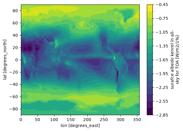
And the LW water vapor kernel, annually and zonally averaged:
data_kern.lw_q.mean(dim=['month', 'lon']).plot.contourf(levels=40, yincrease=False)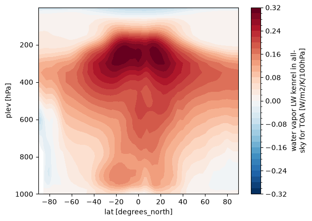
Preparing data for analysis
Define a function for taking global averages:
def global_average(data):
weights = np.cos(np.deg2rad(data.lat))
data_weighted = data.weighted(weights)
return data_weighted.mean(dim=['lat', 'lon'], skipna=True)To get a general idea of how the climate changes in these runs, we can plot the 12-month rolling GMST for the two runs:
gmst_ctrl = global_average(ctrl.tas.rolling(time=12, center=True).mean())gmst_ctrl.sel(time=slice('1150', '1200')).plot()Could not determine bucket type for bucket name cmip6: Your default credentials were not found. To set up Application Default Credentials, see https://cloud.google.com/docs/authentication/external/set-up-adc for more information., falling back to GCSFileSystem
Could not determine bucket type for bucket name cmip6: Your default credentials were not found. To set up Application Default Credentials, see https://cloud.google.com/docs/authentication/external/set-up-adc for more information., falling back to GCSFileSystem
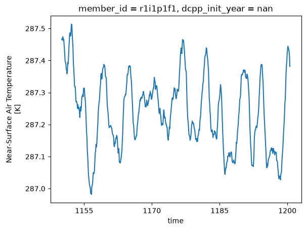
gmst_pert = global_average(pert.tas.rolling(time=12, center=True).mean())gmst_pert.sel(time=slice('0949', '0999')).plot()Could not determine bucket type for bucket name cmip6: Your default credentials were not found. To set up Application Default Credentials, see https://cloud.google.com/docs/authentication/external/set-up-adc for more information., falling back to GCSFileSystem
Could not determine bucket type for bucket name cmip6: Your default credentials were not found. To set up Application Default Credentials, see https://cloud.google.com/docs/authentication/external/set-up-adc for more information., falling back to GCSFileSystem
Could not determine bucket type for bucket name cmip6: Your default credentials were not found. To set up Application Default Credentials, see https://cloud.google.com/docs/authentication/external/set-up-adc for more information., falling back to GCSFileSystem
Could not determine bucket type for bucket name cmip6: Your default credentials were not found. To set up Application Default Credentials, see https://cloud.google.com/docs/authentication/external/set-up-adc for more information., falling back to GCSFileSystem
Could not determine bucket type for bucket name cmip6: Your default credentials were not found. To set up Application Default Credentials, see https://cloud.google.com/docs/authentication/external/set-up-adc for more information., falling back to GCSFileSystem
Could not determine bucket type for bucket name cmip6: Your default credentials were not found. To set up Application Default Credentials, see https://cloud.google.com/docs/authentication/external/set-up-adc for more information., falling back to GCSFileSystem
Could not determine bucket type for bucket name cmip6: Your default credentials were not found. To set up Application Default Credentials, see https://cloud.google.com/docs/authentication/external/set-up-adc for more information., falling back to GCSFileSystem
Could not determine bucket type for bucket name cmip6: Your default credentials were not found. To set up Application Default Credentials, see https://cloud.google.com/docs/authentication/external/set-up-adc for more information., falling back to GCSFileSystem
Could not determine bucket type for bucket name cmip6: Your default credentials were not found. To set up Application Default Credentials, see https://cloud.google.com/docs/authentication/external/set-up-adc for more information., falling back to GCSFileSystem
Could not determine bucket type for bucket name cmip6: Your default credentials were not found. To set up Application Default Credentials, see https://cloud.google.com/docs/authentication/external/set-up-adc for more information., falling back to GCSFileSystem
Could not determine bucket type for bucket name cmip6: Your default credentials were not found. To set up Application Default Credentials, see https://cloud.google.com/docs/authentication/external/set-up-adc for more information., falling back to GCSFileSystem
Could not determine bucket type for bucket name cmip6: Your default credentials were not found. To set up Application Default Credentials, see https://cloud.google.com/docs/authentication/external/set-up-adc for more information., falling back to GCSFileSystem
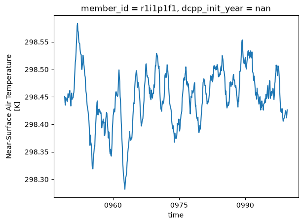
Calculating the two climate states
Ideally, we would want to compare two equilibrated climates, but since that is usually not possible with standard-length CMIP experiments, we will simply use the monthly climatology over the last 50 years available for each run, which is close enough to equilibrium. The pressure coordinates are in Pa, so let’s convert them to hPa to match the kernels:
ctrl_state = ctrl.sel(time=slice('1150', '1200')).groupby('time.month').mean(dim='time').squeeze()
pert_state = pert.sel(time=slice('0949', '0999')).groupby('time.month').mean(dim='time').squeeze()
ctrl_state['plev'] = ctrl_state['plev']/100
pert_state['plev'] = pert_state['plev']/100pert_stateWe will need the change in GMST in order to calculate the feedbacks:
dgmst = global_average(pert_state.tas - ctrl_state.tas).mean(dim='month')
dgmst.load()Could not determine bucket type for bucket name cmip6: Your default credentials were not found. To set up Application Default Credentials, see https://cloud.google.com/docs/authentication/external/set-up-adc for more information., falling back to GCSFileSystem
Could not determine bucket type for bucket name cmip6: Your default credentials were not found. To set up Application Default Credentials, see https://cloud.google.com/docs/authentication/external/set-up-adc for more information., falling back to GCSFileSystem
Could not determine bucket type for bucket name cmip6: Your default credentials were not found. To set up Application Default Credentials, see https://cloud.google.com/docs/authentication/external/set-up-adc for more information., falling back to GCSFileSystem
Could not determine bucket type for bucket name cmip6: Your default credentials were not found. To set up Application Default Credentials, see https://cloud.google.com/docs/authentication/external/set-up-adc for more information., falling back to GCSFileSystem
Could not determine bucket type for bucket name cmip6: Your default credentials were not found. To set up Application Default Credentials, see https://cloud.google.com/docs/authentication/external/set-up-adc for more information., falling back to GCSFileSystem
Could not determine bucket type for bucket name cmip6: Your default credentials were not found. To set up Application Default Credentials, see https://cloud.google.com/docs/authentication/external/set-up-adc for more information., falling back to GCSFileSystem
Could not determine bucket type for bucket name cmip6: Your default credentials were not found. To set up Application Default Credentials, see https://cloud.google.com/docs/authentication/external/set-up-adc for more information., falling back to GCSFileSystem
Could not determine bucket type for bucket name cmip6: Your default credentials were not found. To set up Application Default Credentials, see https://cloud.google.com/docs/authentication/external/set-up-adc for more information., falling back to GCSFileSystem
Could not determine bucket type for bucket name cmip6: Your default credentials were not found. To set up Application Default Credentials, see https://cloud.google.com/docs/authentication/external/set-up-adc for more information., falling back to GCSFileSystem
Could not determine bucket type for bucket name cmip6: Your default credentials were not found. To set up Application Default Credentials, see https://cloud.google.com/docs/authentication/external/set-up-adc for more information., falling back to GCSFileSystem
Could not determine bucket type for bucket name cmip6: Your default credentials were not found. To set up Application Default Credentials, see https://cloud.google.com/docs/authentication/external/set-up-adc for more information., falling back to GCSFileSystem
Could not determine bucket type for bucket name cmip6: Your default credentials were not found. To set up Application Default Credentials, see https://cloud.google.com/docs/authentication/external/set-up-adc for more information., falling back to GCSFileSystem
Could not determine bucket type for bucket name cmip6: Your default credentials were not found. To set up Application Default Credentials, see https://cloud.google.com/docs/authentication/external/set-up-adc for more information., falling back to GCSFileSystem
Could not determine bucket type for bucket name cmip6: Your default credentials were not found. To set up Application Default Credentials, see https://cloud.google.com/docs/authentication/external/set-up-adc for more information., falling back to GCSFileSystem
Regridding
The model output and kernels are not on the same grid, so we will regrid the kernel dataset to the model’s grid using the regridding package xesmf. For reusability, let’s define a function to regrid data:
def regrid(ds_in, regrid_to, method='bilinear'):
regridder = xe.Regridder(ds_in, regrid_to, method=method, periodic=True, ignore_degenerate=True)
ds_out = regridder(ds_in)
return ds_outregr_kernels = regrid(data_kern, pert_state)regr_kernelsCheck that the kernels look as expected:
regr_kernels.sw_a.mean(dim='month').plot.contourf(levels=20)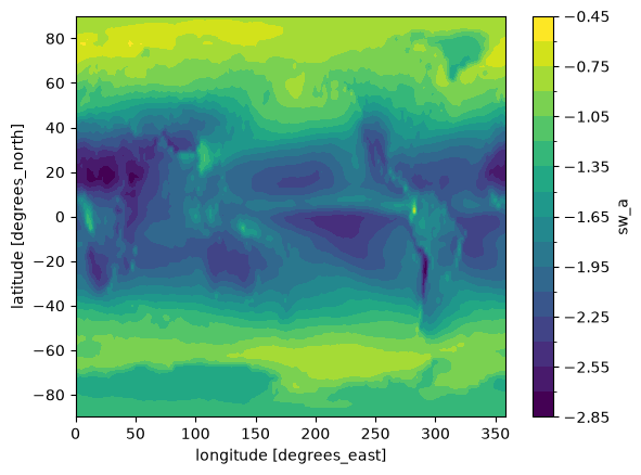
regr_kernels.lw_q.mean(dim=['month', 'lon']).plot.contourf(levels=40, yincrease=False)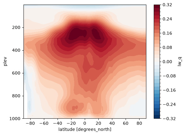
ctrl_state = ctrl_state.interp_like(regr_kernels, kwargs={"fill_value": "extrapolate"})
pert_state = pert_state.interp_like(regr_kernels, kwargs={"fill_value": "extrapolate"})Calculating feedbacks
For all noncloud feedbacks, we will calculate both the all-sky and clear-sky (indicated by clr in the kernel dataset here) change in TOA radiation . For the clear-sky calculations, we just use the clear-sky version of the kernel in place of the all-sky kernel. The differences for each feedback will be used later to adjust the CREs into proper cloud feedbacks.
For the feedbacks involving fields that are a function of pressure (i.e., temperature and water vapor), we need to mask out the stratosphere. In this notebook, we will approximate this using a function that masks above 100 hPa at the equator and linearly decreases to 300 hPa at the poles:
def tropo_mask(ds):
return ds.where(ds.plev > ((200/90)*abs(ds.lat) + 100))Compare:
ctrl_state.ta.mean(dim=['month', 'lon']).plot(yincrease=False)Could not determine bucket type for bucket name cmip6: Your default credentials were not found. To set up Application Default Credentials, see https://cloud.google.com/docs/authentication/external/set-up-adc for more information., falling back to GCSFileSystem
Could not determine bucket type for bucket name cmip6: Your default credentials were not found. To set up Application Default Credentials, see https://cloud.google.com/docs/authentication/external/set-up-adc for more information., falling back to GCSFileSystem
Could not determine bucket type for bucket name cmip6: Your default credentials were not found. To set up Application Default Credentials, see https://cloud.google.com/docs/authentication/external/set-up-adc for more information., falling back to GCSFileSystem
Could not determine bucket type for bucket name cmip6: Your default credentials were not found. To set up Application Default Credentials, see https://cloud.google.com/docs/authentication/external/set-up-adc for more information., falling back to GCSFileSystem
Could not determine bucket type for bucket name cmip6: Your default credentials were not found. To set up Application Default Credentials, see https://cloud.google.com/docs/authentication/external/set-up-adc for more information., falling back to GCSFileSystem
Could not determine bucket type for bucket name cmip6: Your default credentials were not found. To set up Application Default Credentials, see https://cloud.google.com/docs/authentication/external/set-up-adc for more information., falling back to GCSFileSystem
Could not determine bucket type for bucket name cmip6: Your default credentials were not found. To set up Application Default Credentials, see https://cloud.google.com/docs/authentication/external/set-up-adc for more information., falling back to GCSFileSystem
Could not determine bucket type for bucket name cmip6: Your default credentials were not found. To set up Application Default Credentials, see https://cloud.google.com/docs/authentication/external/set-up-adc for more information., falling back to GCSFileSystem
Could not determine bucket type for bucket name cmip6: Your default credentials were not found. To set up Application Default Credentials, see https://cloud.google.com/docs/authentication/external/set-up-adc for more information., falling back to GCSFileSystem
Could not determine bucket type for bucket name cmip6: Your default credentials were not found. To set up Application Default Credentials, see https://cloud.google.com/docs/authentication/external/set-up-adc for more information., falling back to GCSFileSystem
Could not determine bucket type for bucket name cmip6: Your default credentials were not found. To set up Application Default Credentials, see https://cloud.google.com/docs/authentication/external/set-up-adc for more information., falling back to GCSFileSystem
Could not determine bucket type for bucket name cmip6: Your default credentials were not found. To set up Application Default Credentials, see https://cloud.google.com/docs/authentication/external/set-up-adc for more information., falling back to GCSFileSystem
Could not determine bucket type for bucket name cmip6: Your default credentials were not found. To set up Application Default Credentials, see https://cloud.google.com/docs/authentication/external/set-up-adc for more information., falling back to GCSFileSystem
Could not determine bucket type for bucket name cmip6: Your default credentials were not found. To set up Application Default Credentials, see https://cloud.google.com/docs/authentication/external/set-up-adc for more information., falling back to GCSFileSystem
Could not determine bucket type for bucket name cmip6: Your default credentials were not found. To set up Application Default Credentials, see https://cloud.google.com/docs/authentication/external/set-up-adc for more information., falling back to GCSFileSystem
Could not determine bucket type for bucket name cmip6: Your default credentials were not found. To set up Application Default Credentials, see https://cloud.google.com/docs/authentication/external/set-up-adc for more information., falling back to GCSFileSystem
Could not determine bucket type for bucket name cmip6: Your default credentials were not found. To set up Application Default Credentials, see https://cloud.google.com/docs/authentication/external/set-up-adc for more information., falling back to GCSFileSystem
Could not determine bucket type for bucket name cmip6: Your default credentials were not found. To set up Application Default Credentials, see https://cloud.google.com/docs/authentication/external/set-up-adc for more information., falling back to GCSFileSystem
Could not determine bucket type for bucket name cmip6: Your default credentials were not found. To set up Application Default Credentials, see https://cloud.google.com/docs/authentication/external/set-up-adc for more information., falling back to GCSFileSystem
Could not determine bucket type for bucket name cmip6: Your default credentials were not found. To set up Application Default Credentials, see https://cloud.google.com/docs/authentication/external/set-up-adc for more information., falling back to GCSFileSystem
Could not determine bucket type for bucket name cmip6: Your default credentials were not found. To set up Application Default Credentials, see https://cloud.google.com/docs/authentication/external/set-up-adc for more information., falling back to GCSFileSystem
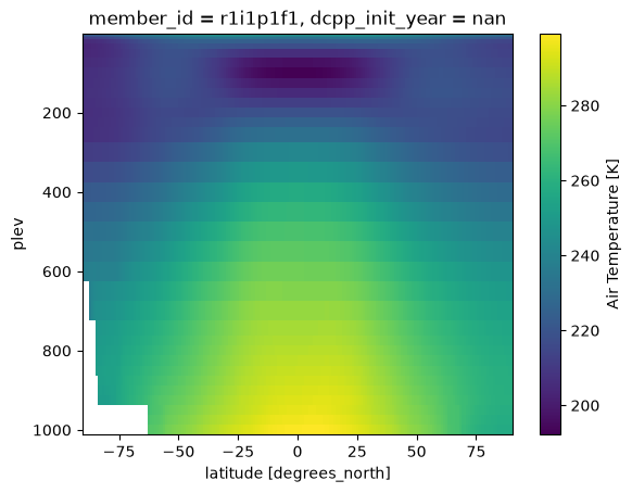
tropo_mask(ctrl_state.ta.mean(dim=['month', 'lon'])).plot(yincrease=False)Could not determine bucket type for bucket name cmip6: Your default credentials were not found. To set up Application Default Credentials, see https://cloud.google.com/docs/authentication/external/set-up-adc for more information., falling back to GCSFileSystem
Could not determine bucket type for bucket name cmip6: Your default credentials were not found. To set up Application Default Credentials, see https://cloud.google.com/docs/authentication/external/set-up-adc for more information., falling back to GCSFileSystem
Could not determine bucket type for bucket name cmip6: Your default credentials were not found. To set up Application Default Credentials, see https://cloud.google.com/docs/authentication/external/set-up-adc for more information., falling back to GCSFileSystem
Could not determine bucket type for bucket name cmip6: Your default credentials were not found. To set up Application Default Credentials, see https://cloud.google.com/docs/authentication/external/set-up-adc for more information., falling back to GCSFileSystem
Could not determine bucket type for bucket name cmip6: Your default credentials were not found. To set up Application Default Credentials, see https://cloud.google.com/docs/authentication/external/set-up-adc for more information., falling back to GCSFileSystem
Could not determine bucket type for bucket name cmip6: Your default credentials were not found. To set up Application Default Credentials, see https://cloud.google.com/docs/authentication/external/set-up-adc for more information., falling back to GCSFileSystem
Could not determine bucket type for bucket name cmip6: Your default credentials were not found. To set up Application Default Credentials, see https://cloud.google.com/docs/authentication/external/set-up-adc for more information., falling back to GCSFileSystem
Could not determine bucket type for bucket name cmip6: Your default credentials were not found. To set up Application Default Credentials, see https://cloud.google.com/docs/authentication/external/set-up-adc for more information., falling back to GCSFileSystem
Could not determine bucket type for bucket name cmip6: Your default credentials were not found. To set up Application Default Credentials, see https://cloud.google.com/docs/authentication/external/set-up-adc for more information., falling back to GCSFileSystem
Could not determine bucket type for bucket name cmip6: Your default credentials were not found. To set up Application Default Credentials, see https://cloud.google.com/docs/authentication/external/set-up-adc for more information., falling back to GCSFileSystem
Could not determine bucket type for bucket name cmip6: Your default credentials were not found. To set up Application Default Credentials, see https://cloud.google.com/docs/authentication/external/set-up-adc for more information., falling back to GCSFileSystem
Could not determine bucket type for bucket name cmip6: Your default credentials were not found. To set up Application Default Credentials, see https://cloud.google.com/docs/authentication/external/set-up-adc for more information., falling back to GCSFileSystem
Could not determine bucket type for bucket name cmip6: Your default credentials were not found. To set up Application Default Credentials, see https://cloud.google.com/docs/authentication/external/set-up-adc for more information., falling back to GCSFileSystem
Could not determine bucket type for bucket name cmip6: Your default credentials were not found. To set up Application Default Credentials, see https://cloud.google.com/docs/authentication/external/set-up-adc for more information., falling back to GCSFileSystem
Could not determine bucket type for bucket name cmip6: Your default credentials were not found. To set up Application Default Credentials, see https://cloud.google.com/docs/authentication/external/set-up-adc for more information., falling back to GCSFileSystem
Could not determine bucket type for bucket name cmip6: Your default credentials were not found. To set up Application Default Credentials, see https://cloud.google.com/docs/authentication/external/set-up-adc for more information., falling back to GCSFileSystem
Could not determine bucket type for bucket name cmip6: Your default credentials were not found. To set up Application Default Credentials, see https://cloud.google.com/docs/authentication/external/set-up-adc for more information., falling back to GCSFileSystem
Could not determine bucket type for bucket name cmip6: Your default credentials were not found. To set up Application Default Credentials, see https://cloud.google.com/docs/authentication/external/set-up-adc for more information., falling back to GCSFileSystem
Could not determine bucket type for bucket name cmip6: Your default credentials were not found. To set up Application Default Credentials, see https://cloud.google.com/docs/authentication/external/set-up-adc for more information., falling back to GCSFileSystem
Could not determine bucket type for bucket name cmip6: Your default credentials were not found. To set up Application Default Credentials, see https://cloud.google.com/docs/authentication/external/set-up-adc for more information., falling back to GCSFileSystem
Could not determine bucket type for bucket name cmip6: Your default credentials were not found. To set up Application Default Credentials, see https://cloud.google.com/docs/authentication/external/set-up-adc for more information., falling back to GCSFileSystem
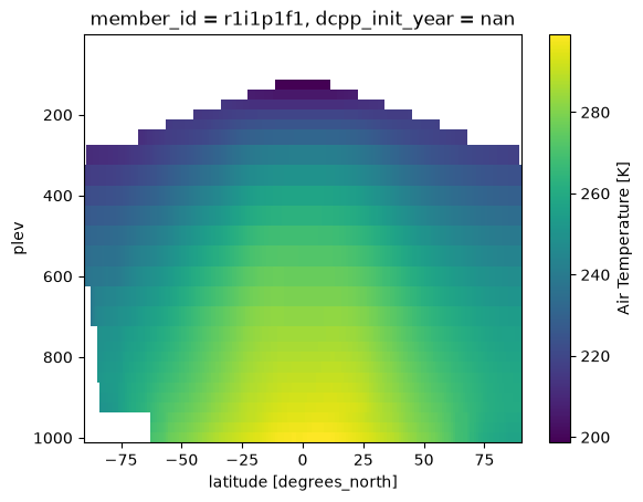
Surface albedo
The first step is to calculate the change in albedo between the control and perturbed climates. The surface albedo is defined as the fraction of downwelling solar radiation at the surface that is reflected back up. That is,
alb_ctrl = (ctrl_state.rsus/ctrl_state.rsds.where(ctrl_state.rsds > 0)).fillna(0)
alb_pert = (pert_state.rsus/pert_state.rsds.where(ctrl_state.rsds > 0)).fillna(0)Note that we avoided dividing by zero by masking regions where rsds = 0 and filling in the resulting nans with 0. Now, take the difference:
dalb = alb_pert - alb_ctrldalb.mean(dim='month').plot()Could not determine bucket type for bucket name cmip6: Your default credentials were not found. To set up Application Default Credentials, see https://cloud.google.com/docs/authentication/external/set-up-adc for more information., falling back to GCSFileSystem
Could not determine bucket type for bucket name cmip6: Your default credentials were not found. To set up Application Default Credentials, see https://cloud.google.com/docs/authentication/external/set-up-adc for more information., falling back to GCSFileSystem
Could not determine bucket type for bucket name cmip6: Your default credentials were not found. To set up Application Default Credentials, see https://cloud.google.com/docs/authentication/external/set-up-adc for more information., falling back to GCSFileSystem
Could not determine bucket type for bucket name cmip6: Your default credentials were not found. To set up Application Default Credentials, see https://cloud.google.com/docs/authentication/external/set-up-adc for more information., falling back to GCSFileSystem
Could not determine bucket type for bucket name cmip6: Your default credentials were not found. To set up Application Default Credentials, see https://cloud.google.com/docs/authentication/external/set-up-adc for more information., falling back to GCSFileSystem
Could not determine bucket type for bucket name cmip6: Your default credentials were not found. To set up Application Default Credentials, see https://cloud.google.com/docs/authentication/external/set-up-adc for more information., falling back to GCSFileSystem
Could not determine bucket type for bucket name cmip6: Your default credentials were not found. To set up Application Default Credentials, see https://cloud.google.com/docs/authentication/external/set-up-adc for more information., falling back to GCSFileSystem
Could not determine bucket type for bucket name cmip6: Your default credentials were not found. To set up Application Default Credentials, see https://cloud.google.com/docs/authentication/external/set-up-adc for more information., falling back to GCSFileSystem
Could not determine bucket type for bucket name cmip6: Your default credentials were not found. To set up Application Default Credentials, see https://cloud.google.com/docs/authentication/external/set-up-adc for more information., falling back to GCSFileSystem
Could not determine bucket type for bucket name cmip6: Your default credentials were not found. To set up Application Default Credentials, see https://cloud.google.com/docs/authentication/external/set-up-adc for more information., falling back to GCSFileSystem
Could not determine bucket type for bucket name cmip6: Your default credentials were not found. To set up Application Default Credentials, see https://cloud.google.com/docs/authentication/external/set-up-adc for more information., falling back to GCSFileSystem
Could not determine bucket type for bucket name cmip6: Your default credentials were not found. To set up Application Default Credentials, see https://cloud.google.com/docs/authentication/external/set-up-adc for more information., falling back to GCSFileSystem
Could not determine bucket type for bucket name cmip6: Your default credentials were not found. To set up Application Default Credentials, see https://cloud.google.com/docs/authentication/external/set-up-adc for more information., falling back to GCSFileSystem
Could not determine bucket type for bucket name cmip6: Your default credentials were not found. To set up Application Default Credentials, see https://cloud.google.com/docs/authentication/external/set-up-adc for more information., falling back to GCSFileSystem
Could not determine bucket type for bucket name cmip6: Your default credentials were not found. To set up Application Default Credentials, see https://cloud.google.com/docs/authentication/external/set-up-adc for more information., falling back to GCSFileSystem
Could not determine bucket type for bucket name cmip6: Your default credentials were not found. To set up Application Default Credentials, see https://cloud.google.com/docs/authentication/external/set-up-adc for more information., falling back to GCSFileSystem
Could not determine bucket type for bucket name cmip6: Your default credentials were not found. To set up Application Default Credentials, see https://cloud.google.com/docs/authentication/external/set-up-adc for more information., falling back to GCSFileSystem
Could not determine bucket type for bucket name cmip6: Your default credentials were not found. To set up Application Default Credentials, see https://cloud.google.com/docs/authentication/external/set-up-adc for more information., falling back to GCSFileSystem
Could not determine bucket type for bucket name cmip6: Your default credentials were not found. To set up Application Default Credentials, see https://cloud.google.com/docs/authentication/external/set-up-adc for more information., falling back to GCSFileSystem
Could not determine bucket type for bucket name cmip6: Your default credentials were not found. To set up Application Default Credentials, see https://cloud.google.com/docs/authentication/external/set-up-adc for more information., falling back to GCSFileSystem
Could not determine bucket type for bucket name cmip6: Your default credentials were not found. To set up Application Default Credentials, see https://cloud.google.com/docs/authentication/external/set-up-adc for more information., falling back to GCSFileSystem
Could not determine bucket type for bucket name cmip6: Your default credentials were not found. To set up Application Default Credentials, see https://cloud.google.com/docs/authentication/external/set-up-adc for more information., falling back to GCSFileSystem
Could not determine bucket type for bucket name cmip6: Your default credentials were not found. To set up Application Default Credentials, see https://cloud.google.com/docs/authentication/external/set-up-adc for more information., falling back to GCSFileSystem
Could not determine bucket type for bucket name cmip6: Your default credentials were not found. To set up Application Default Credentials, see https://cloud.google.com/docs/authentication/external/set-up-adc for more information., falling back to GCSFileSystem
Could not determine bucket type for bucket name cmip6: Your default credentials were not found. To set up Application Default Credentials, see https://cloud.google.com/docs/authentication/external/set-up-adc for more information., falling back to GCSFileSystem
Could not determine bucket type for bucket name cmip6: Your default credentials were not found. To set up Application Default Credentials, see https://cloud.google.com/docs/authentication/external/set-up-adc for more information., falling back to GCSFileSystem
Could not determine bucket type for bucket name cmip6: Your default credentials were not found. To set up Application Default Credentials, see https://cloud.google.com/docs/authentication/external/set-up-adc for more information., falling back to GCSFileSystem
Could not determine bucket type for bucket name cmip6: Your default credentials were not found. To set up Application Default Credentials, see https://cloud.google.com/docs/authentication/external/set-up-adc for more information., falling back to GCSFileSystem
Could not determine bucket type for bucket name cmip6: Your default credentials were not found. To set up Application Default Credentials, see https://cloud.google.com/docs/authentication/external/set-up-adc for more information., falling back to GCSFileSystem
Could not determine bucket type for bucket name cmip6: Your default credentials were not found. To set up Application Default Credentials, see https://cloud.google.com/docs/authentication/external/set-up-adc for more information., falling back to GCSFileSystem
Could not determine bucket type for bucket name cmip6: Your default credentials were not found. To set up Application Default Credentials, see https://cloud.google.com/docs/authentication/external/set-up-adc for more information., falling back to GCSFileSystem
Could not determine bucket type for bucket name cmip6: Your default credentials were not found. To set up Application Default Credentials, see https://cloud.google.com/docs/authentication/external/set-up-adc for more information., falling back to GCSFileSystem
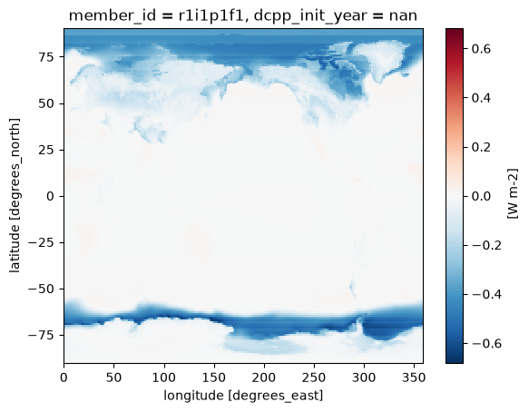
By multiplying the change in albedo with the albedo kernel, we get the change in TOA radiation (in units W m) resulting from that change in albedo:
We also need to multiply by 100 to get albedo as a percentage.
dSW_alb = regr_kernels.sw_a * dalb * 100
dSW_alb = dSW_alb.where(dSW_alb != float('-inf'), np.nan)
dSW_alb_clr = regr_kernels.swclr_a * dalb * 100
dSW_alb_clr = dSW_alb_clr.where(dSW_alb != float('-inf'), np.nan)dSW_alb.mean(dim='month').plot()Could not determine bucket type for bucket name cmip6: Your default credentials were not found. To set up Application Default Credentials, see https://cloud.google.com/docs/authentication/external/set-up-adc for more information., falling back to GCSFileSystem
Could not determine bucket type for bucket name cmip6: Your default credentials were not found. To set up Application Default Credentials, see https://cloud.google.com/docs/authentication/external/set-up-adc for more information., falling back to GCSFileSystem
Could not determine bucket type for bucket name cmip6: Your default credentials were not found. To set up Application Default Credentials, see https://cloud.google.com/docs/authentication/external/set-up-adc for more information., falling back to GCSFileSystem
Could not determine bucket type for bucket name cmip6: Your default credentials were not found. To set up Application Default Credentials, see https://cloud.google.com/docs/authentication/external/set-up-adc for more information., falling back to GCSFileSystem
Could not determine bucket type for bucket name cmip6: Your default credentials were not found. To set up Application Default Credentials, see https://cloud.google.com/docs/authentication/external/set-up-adc for more information., falling back to GCSFileSystem
Could not determine bucket type for bucket name cmip6: Your default credentials were not found. To set up Application Default Credentials, see https://cloud.google.com/docs/authentication/external/set-up-adc for more information., falling back to GCSFileSystem
Could not determine bucket type for bucket name cmip6: Your default credentials were not found. To set up Application Default Credentials, see https://cloud.google.com/docs/authentication/external/set-up-adc for more information., falling back to GCSFileSystem
Could not determine bucket type for bucket name cmip6: Your default credentials were not found. To set up Application Default Credentials, see https://cloud.google.com/docs/authentication/external/set-up-adc for more information., falling back to GCSFileSystem
Could not determine bucket type for bucket name cmip6: Your default credentials were not found. To set up Application Default Credentials, see https://cloud.google.com/docs/authentication/external/set-up-adc for more information., falling back to GCSFileSystem
Could not determine bucket type for bucket name cmip6: Your default credentials were not found. To set up Application Default Credentials, see https://cloud.google.com/docs/authentication/external/set-up-adc for more information., falling back to GCSFileSystem
Could not determine bucket type for bucket name cmip6: Your default credentials were not found. To set up Application Default Credentials, see https://cloud.google.com/docs/authentication/external/set-up-adc for more information., falling back to GCSFileSystem
Could not determine bucket type for bucket name cmip6: Your default credentials were not found. To set up Application Default Credentials, see https://cloud.google.com/docs/authentication/external/set-up-adc for more information., falling back to GCSFileSystem
Could not determine bucket type for bucket name cmip6: Your default credentials were not found. To set up Application Default Credentials, see https://cloud.google.com/docs/authentication/external/set-up-adc for more information., falling back to GCSFileSystem
Could not determine bucket type for bucket name cmip6: Your default credentials were not found. To set up Application Default Credentials, see https://cloud.google.com/docs/authentication/external/set-up-adc for more information., falling back to GCSFileSystem
Could not determine bucket type for bucket name cmip6: Your default credentials were not found. To set up Application Default Credentials, see https://cloud.google.com/docs/authentication/external/set-up-adc for more information., falling back to GCSFileSystem
Could not determine bucket type for bucket name cmip6: Your default credentials were not found. To set up Application Default Credentials, see https://cloud.google.com/docs/authentication/external/set-up-adc for more information., falling back to GCSFileSystem
Could not determine bucket type for bucket name cmip6: Your default credentials were not found. To set up Application Default Credentials, see https://cloud.google.com/docs/authentication/external/set-up-adc for more information., falling back to GCSFileSystem
Could not determine bucket type for bucket name cmip6: Your default credentials were not found. To set up Application Default Credentials, see https://cloud.google.com/docs/authentication/external/set-up-adc for more information., falling back to GCSFileSystem
Could not determine bucket type for bucket name cmip6: Your default credentials were not found. To set up Application Default Credentials, see https://cloud.google.com/docs/authentication/external/set-up-adc for more information., falling back to GCSFileSystem
Could not determine bucket type for bucket name cmip6: Your default credentials were not found. To set up Application Default Credentials, see https://cloud.google.com/docs/authentication/external/set-up-adc for more information., falling back to GCSFileSystem
Could not determine bucket type for bucket name cmip6: Your default credentials were not found. To set up Application Default Credentials, see https://cloud.google.com/docs/authentication/external/set-up-adc for more information., falling back to GCSFileSystem
Could not determine bucket type for bucket name cmip6: Your default credentials were not found. To set up Application Default Credentials, see https://cloud.google.com/docs/authentication/external/set-up-adc for more information., falling back to GCSFileSystem
Could not determine bucket type for bucket name cmip6: Your default credentials were not found. To set up Application Default Credentials, see https://cloud.google.com/docs/authentication/external/set-up-adc for more information., falling back to GCSFileSystem
Could not determine bucket type for bucket name cmip6: Your default credentials were not found. To set up Application Default Credentials, see https://cloud.google.com/docs/authentication/external/set-up-adc for more information., falling back to GCSFileSystem
Could not determine bucket type for bucket name cmip6: Your default credentials were not found. To set up Application Default Credentials, see https://cloud.google.com/docs/authentication/external/set-up-adc for more information., falling back to GCSFileSystem
Could not determine bucket type for bucket name cmip6: Your default credentials were not found. To set up Application Default Credentials, see https://cloud.google.com/docs/authentication/external/set-up-adc for more information., falling back to GCSFileSystem
Could not determine bucket type for bucket name cmip6: Your default credentials were not found. To set up Application Default Credentials, see https://cloud.google.com/docs/authentication/external/set-up-adc for more information., falling back to GCSFileSystem
Could not determine bucket type for bucket name cmip6: Your default credentials were not found. To set up Application Default Credentials, see https://cloud.google.com/docs/authentication/external/set-up-adc for more information., falling back to GCSFileSystem
Could not determine bucket type for bucket name cmip6: Your default credentials were not found. To set up Application Default Credentials, see https://cloud.google.com/docs/authentication/external/set-up-adc for more information., falling back to GCSFileSystem
Could not determine bucket type for bucket name cmip6: Your default credentials were not found. To set up Application Default Credentials, see https://cloud.google.com/docs/authentication/external/set-up-adc for more information., falling back to GCSFileSystem
Could not determine bucket type for bucket name cmip6: Your default credentials were not found. To set up Application Default Credentials, see https://cloud.google.com/docs/authentication/external/set-up-adc for more information., falling back to GCSFileSystem
Could not determine bucket type for bucket name cmip6: Your default credentials were not found. To set up Application Default Credentials, see https://cloud.google.com/docs/authentication/external/set-up-adc for more information., falling back to GCSFileSystem
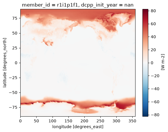
The feedback in units W m K is then calculated by normalizing this change in TOA radiation by the change in GMST:
alb_feedback = dSW_alb/dgmstalb_feedback.mean(dim='month').plot()Could not determine bucket type for bucket name cmip6: Your default credentials were not found. To set up Application Default Credentials, see https://cloud.google.com/docs/authentication/external/set-up-adc for more information., falling back to GCSFileSystem
Could not determine bucket type for bucket name cmip6: Your default credentials were not found. To set up Application Default Credentials, see https://cloud.google.com/docs/authentication/external/set-up-adc for more information., falling back to GCSFileSystem
Could not determine bucket type for bucket name cmip6: Your default credentials were not found. To set up Application Default Credentials, see https://cloud.google.com/docs/authentication/external/set-up-adc for more information., falling back to GCSFileSystem
Could not determine bucket type for bucket name cmip6: Your default credentials were not found. To set up Application Default Credentials, see https://cloud.google.com/docs/authentication/external/set-up-adc for more information., falling back to GCSFileSystem
Could not determine bucket type for bucket name cmip6: Your default credentials were not found. To set up Application Default Credentials, see https://cloud.google.com/docs/authentication/external/set-up-adc for more information., falling back to GCSFileSystem
Could not determine bucket type for bucket name cmip6: Your default credentials were not found. To set up Application Default Credentials, see https://cloud.google.com/docs/authentication/external/set-up-adc for more information., falling back to GCSFileSystem
Could not determine bucket type for bucket name cmip6: Your default credentials were not found. To set up Application Default Credentials, see https://cloud.google.com/docs/authentication/external/set-up-adc for more information., falling back to GCSFileSystem
Could not determine bucket type for bucket name cmip6: Your default credentials were not found. To set up Application Default Credentials, see https://cloud.google.com/docs/authentication/external/set-up-adc for more information., falling back to GCSFileSystem
Could not determine bucket type for bucket name cmip6: Your default credentials were not found. To set up Application Default Credentials, see https://cloud.google.com/docs/authentication/external/set-up-adc for more information., falling back to GCSFileSystem
Could not determine bucket type for bucket name cmip6: Your default credentials were not found. To set up Application Default Credentials, see https://cloud.google.com/docs/authentication/external/set-up-adc for more information., falling back to GCSFileSystem
Could not determine bucket type for bucket name cmip6: Your default credentials were not found. To set up Application Default Credentials, see https://cloud.google.com/docs/authentication/external/set-up-adc for more information., falling back to GCSFileSystem
Could not determine bucket type for bucket name cmip6: Your default credentials were not found. To set up Application Default Credentials, see https://cloud.google.com/docs/authentication/external/set-up-adc for more information., falling back to GCSFileSystem
Could not determine bucket type for bucket name cmip6: Your default credentials were not found. To set up Application Default Credentials, see https://cloud.google.com/docs/authentication/external/set-up-adc for more information., falling back to GCSFileSystem
Could not determine bucket type for bucket name cmip6: Your default credentials were not found. To set up Application Default Credentials, see https://cloud.google.com/docs/authentication/external/set-up-adc for more information., falling back to GCSFileSystem
Could not determine bucket type for bucket name cmip6: Your default credentials were not found. To set up Application Default Credentials, see https://cloud.google.com/docs/authentication/external/set-up-adc for more information., falling back to GCSFileSystem
Could not determine bucket type for bucket name cmip6: Your default credentials were not found. To set up Application Default Credentials, see https://cloud.google.com/docs/authentication/external/set-up-adc for more information., falling back to GCSFileSystem
Could not determine bucket type for bucket name cmip6: Your default credentials were not found. To set up Application Default Credentials, see https://cloud.google.com/docs/authentication/external/set-up-adc for more information., falling back to GCSFileSystem
Could not determine bucket type for bucket name cmip6: Your default credentials were not found. To set up Application Default Credentials, see https://cloud.google.com/docs/authentication/external/set-up-adc for more information., falling back to GCSFileSystem
Could not determine bucket type for bucket name cmip6: Your default credentials were not found. To set up Application Default Credentials, see https://cloud.google.com/docs/authentication/external/set-up-adc for more information., falling back to GCSFileSystem
Could not determine bucket type for bucket name cmip6: Your default credentials were not found. To set up Application Default Credentials, see https://cloud.google.com/docs/authentication/external/set-up-adc for more information., falling back to GCSFileSystem
Could not determine bucket type for bucket name cmip6: Your default credentials were not found. To set up Application Default Credentials, see https://cloud.google.com/docs/authentication/external/set-up-adc for more information., falling back to GCSFileSystem
Could not determine bucket type for bucket name cmip6: Your default credentials were not found. To set up Application Default Credentials, see https://cloud.google.com/docs/authentication/external/set-up-adc for more information., falling back to GCSFileSystem
Could not determine bucket type for bucket name cmip6: Your default credentials were not found. To set up Application Default Credentials, see https://cloud.google.com/docs/authentication/external/set-up-adc for more information., falling back to GCSFileSystem
Could not determine bucket type for bucket name cmip6: Your default credentials were not found. To set up Application Default Credentials, see https://cloud.google.com/docs/authentication/external/set-up-adc for more information., falling back to GCSFileSystem
Could not determine bucket type for bucket name cmip6: Your default credentials were not found. To set up Application Default Credentials, see https://cloud.google.com/docs/authentication/external/set-up-adc for more information., falling back to GCSFileSystem
Could not determine bucket type for bucket name cmip6: Your default credentials were not found. To set up Application Default Credentials, see https://cloud.google.com/docs/authentication/external/set-up-adc for more information., falling back to GCSFileSystem
Could not determine bucket type for bucket name cmip6: Your default credentials were not found. To set up Application Default Credentials, see https://cloud.google.com/docs/authentication/external/set-up-adc for more information., falling back to GCSFileSystem
Could not determine bucket type for bucket name cmip6: Your default credentials were not found. To set up Application Default Credentials, see https://cloud.google.com/docs/authentication/external/set-up-adc for more information., falling back to GCSFileSystem
Could not determine bucket type for bucket name cmip6: Your default credentials were not found. To set up Application Default Credentials, see https://cloud.google.com/docs/authentication/external/set-up-adc for more information., falling back to GCSFileSystem
Could not determine bucket type for bucket name cmip6: Your default credentials were not found. To set up Application Default Credentials, see https://cloud.google.com/docs/authentication/external/set-up-adc for more information., falling back to GCSFileSystem
Could not determine bucket type for bucket name cmip6: Your default credentials were not found. To set up Application Default Credentials, see https://cloud.google.com/docs/authentication/external/set-up-adc for more information., falling back to GCSFileSystem
Could not determine bucket type for bucket name cmip6: Your default credentials were not found. To set up Application Default Credentials, see https://cloud.google.com/docs/authentication/external/set-up-adc for more information., falling back to GCSFileSystem
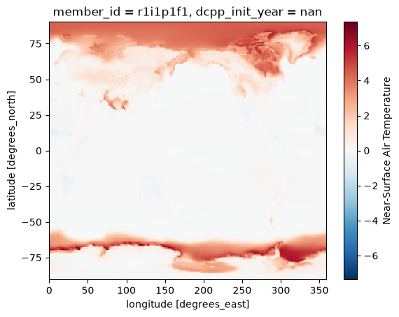
Taking the global and annual average, we get a final value of:
global_average(alb_feedback.mean(dim='month')).load()Could not determine bucket type for bucket name cmip6: Your default credentials were not found. To set up Application Default Credentials, see https://cloud.google.com/docs/authentication/external/set-up-adc for more information., falling back to GCSFileSystem
Could not determine bucket type for bucket name cmip6: Your default credentials were not found. To set up Application Default Credentials, see https://cloud.google.com/docs/authentication/external/set-up-adc for more information., falling back to GCSFileSystem
Could not determine bucket type for bucket name cmip6: Your default credentials were not found. To set up Application Default Credentials, see https://cloud.google.com/docs/authentication/external/set-up-adc for more information., falling back to GCSFileSystem
Could not determine bucket type for bucket name cmip6: Your default credentials were not found. To set up Application Default Credentials, see https://cloud.google.com/docs/authentication/external/set-up-adc for more information., falling back to GCSFileSystem
Could not determine bucket type for bucket name cmip6: Your default credentials were not found. To set up Application Default Credentials, see https://cloud.google.com/docs/authentication/external/set-up-adc for more information., falling back to GCSFileSystem
Could not determine bucket type for bucket name cmip6: Your default credentials were not found. To set up Application Default Credentials, see https://cloud.google.com/docs/authentication/external/set-up-adc for more information., falling back to GCSFileSystem
Could not determine bucket type for bucket name cmip6: Your default credentials were not found. To set up Application Default Credentials, see https://cloud.google.com/docs/authentication/external/set-up-adc for more information., falling back to GCSFileSystem
Could not determine bucket type for bucket name cmip6: Your default credentials were not found. To set up Application Default Credentials, see https://cloud.google.com/docs/authentication/external/set-up-adc for more information., falling back to GCSFileSystem
Could not determine bucket type for bucket name cmip6: Your default credentials were not found. To set up Application Default Credentials, see https://cloud.google.com/docs/authentication/external/set-up-adc for more information., falling back to GCSFileSystem
Could not determine bucket type for bucket name cmip6: Your default credentials were not found. To set up Application Default Credentials, see https://cloud.google.com/docs/authentication/external/set-up-adc for more information., falling back to GCSFileSystem
Could not determine bucket type for bucket name cmip6: Your default credentials were not found. To set up Application Default Credentials, see https://cloud.google.com/docs/authentication/external/set-up-adc for more information., falling back to GCSFileSystem
Could not determine bucket type for bucket name cmip6: Your default credentials were not found. To set up Application Default Credentials, see https://cloud.google.com/docs/authentication/external/set-up-adc for more information., falling back to GCSFileSystem
Could not determine bucket type for bucket name cmip6: Your default credentials were not found. To set up Application Default Credentials, see https://cloud.google.com/docs/authentication/external/set-up-adc for more information., falling back to GCSFileSystem
Could not determine bucket type for bucket name cmip6: Your default credentials were not found. To set up Application Default Credentials, see https://cloud.google.com/docs/authentication/external/set-up-adc for more information., falling back to GCSFileSystem
Could not determine bucket type for bucket name cmip6: Your default credentials were not found. To set up Application Default Credentials, see https://cloud.google.com/docs/authentication/external/set-up-adc for more information., falling back to GCSFileSystem
Could not determine bucket type for bucket name cmip6: Your default credentials were not found. To set up Application Default Credentials, see https://cloud.google.com/docs/authentication/external/set-up-adc for more information., falling back to GCSFileSystem
Could not determine bucket type for bucket name cmip6: Your default credentials were not found. To set up Application Default Credentials, see https://cloud.google.com/docs/authentication/external/set-up-adc for more information., falling back to GCSFileSystem
Could not determine bucket type for bucket name cmip6: Your default credentials were not found. To set up Application Default Credentials, see https://cloud.google.com/docs/authentication/external/set-up-adc for more information., falling back to GCSFileSystem
Could not determine bucket type for bucket name cmip6: Your default credentials were not found. To set up Application Default Credentials, see https://cloud.google.com/docs/authentication/external/set-up-adc for more information., falling back to GCSFileSystem
Could not determine bucket type for bucket name cmip6: Your default credentials were not found. To set up Application Default Credentials, see https://cloud.google.com/docs/authentication/external/set-up-adc for more information., falling back to GCSFileSystem
Could not determine bucket type for bucket name cmip6: Your default credentials were not found. To set up Application Default Credentials, see https://cloud.google.com/docs/authentication/external/set-up-adc for more information., falling back to GCSFileSystem
Could not determine bucket type for bucket name cmip6: Your default credentials were not found. To set up Application Default Credentials, see https://cloud.google.com/docs/authentication/external/set-up-adc for more information., falling back to GCSFileSystem
Could not determine bucket type for bucket name cmip6: Your default credentials were not found. To set up Application Default Credentials, see https://cloud.google.com/docs/authentication/external/set-up-adc for more information., falling back to GCSFileSystem
Could not determine bucket type for bucket name cmip6: Your default credentials were not found. To set up Application Default Credentials, see https://cloud.google.com/docs/authentication/external/set-up-adc for more information., falling back to GCSFileSystem
Could not determine bucket type for bucket name cmip6: Your default credentials were not found. To set up Application Default Credentials, see https://cloud.google.com/docs/authentication/external/set-up-adc for more information., falling back to GCSFileSystem
Could not determine bucket type for bucket name cmip6: Your default credentials were not found. To set up Application Default Credentials, see https://cloud.google.com/docs/authentication/external/set-up-adc for more information., falling back to GCSFileSystem
Could not determine bucket type for bucket name cmip6: Your default credentials were not found. To set up Application Default Credentials, see https://cloud.google.com/docs/authentication/external/set-up-adc for more information., falling back to GCSFileSystem
Could not determine bucket type for bucket name cmip6: Your default credentials were not found. To set up Application Default Credentials, see https://cloud.google.com/docs/authentication/external/set-up-adc for more information., falling back to GCSFileSystem
Could not determine bucket type for bucket name cmip6: Your default credentials were not found. To set up Application Default Credentials, see https://cloud.google.com/docs/authentication/external/set-up-adc for more information., falling back to GCSFileSystem
Could not determine bucket type for bucket name cmip6: Your default credentials were not found. To set up Application Default Credentials, see https://cloud.google.com/docs/authentication/external/set-up-adc for more information., falling back to GCSFileSystem
Could not determine bucket type for bucket name cmip6: Your default credentials were not found. To set up Application Default Credentials, see https://cloud.google.com/docs/authentication/external/set-up-adc for more information., falling back to GCSFileSystem
Could not determine bucket type for bucket name cmip6: Your default credentials were not found. To set up Application Default Credentials, see https://cloud.google.com/docs/authentication/external/set-up-adc for more information., falling back to GCSFileSystem
Temperature
The temperature feedback is decomposed into Planck and lapse rate feedbacks, but first, we can calculate the change in TOA LW radiation resulting from changes in surface (ts) and air (ta) temperature. The first step is calculating the changes in surface and air temperature. At the same time, we will interpolate ta to the kernel pressure levels:
dts = pert_state.ts - ctrl_state.ts
dta = pert_state.ta - ctrl_state.taApproximate layer thickness:
dp = -dta.plev.diff(dim='plev', label='lower')
dpThen the change in TOA radiation using the kernels:
And for feedbacks that involve functions of pressure, we integrate (sum) over the pressure levels. These kernels have units W m K (100 hPa), so if is in hPa,
dLW_ts = regr_kernels.lw_ts * dts
dLW_ts_clr = regr_kernels.lwclr_ts * dts
dLW_ta = (regr_kernels.lw_t * tropo_mask(dta) * dp/100).sum(dim='plev', skipna=True)
dLW_ta_clr = (regr_kernels.lwclr_t * tropo_mask(dta) * dp/100).sum(dim='plev', skipna=True)dLW_ts.mean(dim='month').plot()Could not determine bucket type for bucket name cmip6: Your default credentials were not found. To set up Application Default Credentials, see https://cloud.google.com/docs/authentication/external/set-up-adc for more information., falling back to GCSFileSystem
Could not determine bucket type for bucket name cmip6: Your default credentials were not found. To set up Application Default Credentials, see https://cloud.google.com/docs/authentication/external/set-up-adc for more information., falling back to GCSFileSystem
Could not determine bucket type for bucket name cmip6: Your default credentials were not found. To set up Application Default Credentials, see https://cloud.google.com/docs/authentication/external/set-up-adc for more information., falling back to GCSFileSystem
Could not determine bucket type for bucket name cmip6: Your default credentials were not found. To set up Application Default Credentials, see https://cloud.google.com/docs/authentication/external/set-up-adc for more information., falling back to GCSFileSystem
Could not determine bucket type for bucket name cmip6: Your default credentials were not found. To set up Application Default Credentials, see https://cloud.google.com/docs/authentication/external/set-up-adc for more information., falling back to GCSFileSystem
Could not determine bucket type for bucket name cmip6: Your default credentials were not found. To set up Application Default Credentials, see https://cloud.google.com/docs/authentication/external/set-up-adc for more information., falling back to GCSFileSystem
Could not determine bucket type for bucket name cmip6: Your default credentials were not found. To set up Application Default Credentials, see https://cloud.google.com/docs/authentication/external/set-up-adc for more information., falling back to GCSFileSystem
Could not determine bucket type for bucket name cmip6: Your default credentials were not found. To set up Application Default Credentials, see https://cloud.google.com/docs/authentication/external/set-up-adc for more information., falling back to GCSFileSystem
Could not determine bucket type for bucket name cmip6: Your default credentials were not found. To set up Application Default Credentials, see https://cloud.google.com/docs/authentication/external/set-up-adc for more information., falling back to GCSFileSystem
Could not determine bucket type for bucket name cmip6: Your default credentials were not found. To set up Application Default Credentials, see https://cloud.google.com/docs/authentication/external/set-up-adc for more information., falling back to GCSFileSystem
Could not determine bucket type for bucket name cmip6: Your default credentials were not found. To set up Application Default Credentials, see https://cloud.google.com/docs/authentication/external/set-up-adc for more information., falling back to GCSFileSystem
Could not determine bucket type for bucket name cmip6: Your default credentials were not found. To set up Application Default Credentials, see https://cloud.google.com/docs/authentication/external/set-up-adc for more information., falling back to GCSFileSystem
Could not determine bucket type for bucket name cmip6: Your default credentials were not found. To set up Application Default Credentials, see https://cloud.google.com/docs/authentication/external/set-up-adc for more information., falling back to GCSFileSystem
Could not determine bucket type for bucket name cmip6: Your default credentials were not found. To set up Application Default Credentials, see https://cloud.google.com/docs/authentication/external/set-up-adc for more information., falling back to GCSFileSystem
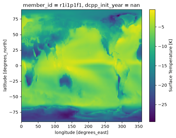
dLW_ta.mean(dim='month').plot()Could not determine bucket type for bucket name cmip6: Your default credentials were not found. To set up Application Default Credentials, see https://cloud.google.com/docs/authentication/external/set-up-adc for more information., falling back to GCSFileSystem
Could not determine bucket type for bucket name cmip6: Your default credentials were not found. To set up Application Default Credentials, see https://cloud.google.com/docs/authentication/external/set-up-adc for more information., falling back to GCSFileSystem
Could not determine bucket type for bucket name cmip6: Your default credentials were not found. To set up Application Default Credentials, see https://cloud.google.com/docs/authentication/external/set-up-adc for more information., falling back to GCSFileSystem
Could not determine bucket type for bucket name cmip6: Your default credentials were not found. To set up Application Default Credentials, see https://cloud.google.com/docs/authentication/external/set-up-adc for more information., falling back to GCSFileSystem
Could not determine bucket type for bucket name cmip6: Your default credentials were not found. To set up Application Default Credentials, see https://cloud.google.com/docs/authentication/external/set-up-adc for more information., falling back to GCSFileSystem
Could not determine bucket type for bucket name cmip6: Your default credentials were not found. To set up Application Default Credentials, see https://cloud.google.com/docs/authentication/external/set-up-adc for more information., falling back to GCSFileSystem
Could not determine bucket type for bucket name cmip6: Your default credentials were not found. To set up Application Default Credentials, see https://cloud.google.com/docs/authentication/external/set-up-adc for more information., falling back to GCSFileSystem
Could not determine bucket type for bucket name cmip6: Your default credentials were not found. To set up Application Default Credentials, see https://cloud.google.com/docs/authentication/external/set-up-adc for more information., falling back to GCSFileSystem
Could not determine bucket type for bucket name cmip6: Your default credentials were not found. To set up Application Default Credentials, see https://cloud.google.com/docs/authentication/external/set-up-adc for more information., falling back to GCSFileSystem
Could not determine bucket type for bucket name cmip6: Your default credentials were not found. To set up Application Default Credentials, see https://cloud.google.com/docs/authentication/external/set-up-adc for more information., falling back to GCSFileSystem
Could not determine bucket type for bucket name cmip6: Your default credentials were not found. To set up Application Default Credentials, see https://cloud.google.com/docs/authentication/external/set-up-adc for more information., falling back to GCSFileSystem
Could not determine bucket type for bucket name cmip6: Your default credentials were not found. To set up Application Default Credentials, see https://cloud.google.com/docs/authentication/external/set-up-adc for more information., falling back to GCSFileSystem
Could not determine bucket type for bucket name cmip6: Your default credentials were not found. To set up Application Default Credentials, see https://cloud.google.com/docs/authentication/external/set-up-adc for more information., falling back to GCSFileSystem
Could not determine bucket type for bucket name cmip6: Your default credentials were not found. To set up Application Default Credentials, see https://cloud.google.com/docs/authentication/external/set-up-adc for more information., falling back to GCSFileSystem
Could not determine bucket type for bucket name cmip6: Your default credentials were not found. To set up Application Default Credentials, see https://cloud.google.com/docs/authentication/external/set-up-adc for more information., falling back to GCSFileSystem
Could not determine bucket type for bucket name cmip6: Your default credentials were not found. To set up Application Default Credentials, see https://cloud.google.com/docs/authentication/external/set-up-adc for more information., falling back to GCSFileSystem
Could not determine bucket type for bucket name cmip6: Your default credentials were not found. To set up Application Default Credentials, see https://cloud.google.com/docs/authentication/external/set-up-adc for more information., falling back to GCSFileSystem
Could not determine bucket type for bucket name cmip6: Your default credentials were not found. To set up Application Default Credentials, see https://cloud.google.com/docs/authentication/external/set-up-adc for more information., falling back to GCSFileSystem
Could not determine bucket type for bucket name cmip6: Your default credentials were not found. To set up Application Default Credentials, see https://cloud.google.com/docs/authentication/external/set-up-adc for more information., falling back to GCSFileSystem
Could not determine bucket type for bucket name cmip6: Your default credentials were not found. To set up Application Default Credentials, see https://cloud.google.com/docs/authentication/external/set-up-adc for more information., falling back to GCSFileSystem
Could not determine bucket type for bucket name cmip6: Your default credentials were not found. To set up Application Default Credentials, see https://cloud.google.com/docs/authentication/external/set-up-adc for more information., falling back to GCSFileSystem
Could not determine bucket type for bucket name cmip6: Your default credentials were not found. To set up Application Default Credentials, see https://cloud.google.com/docs/authentication/external/set-up-adc for more information., falling back to GCSFileSystem
Could not determine bucket type for bucket name cmip6: Your default credentials were not found. To set up Application Default Credentials, see https://cloud.google.com/docs/authentication/external/set-up-adc for more information., falling back to GCSFileSystem
Could not determine bucket type for bucket name cmip6: Your default credentials were not found. To set up Application Default Credentials, see https://cloud.google.com/docs/authentication/external/set-up-adc for more information., falling back to GCSFileSystem
Could not determine bucket type for bucket name cmip6: Your default credentials were not found. To set up Application Default Credentials, see https://cloud.google.com/docs/authentication/external/set-up-adc for more information., falling back to GCSFileSystem
Could not determine bucket type for bucket name cmip6: Your default credentials were not found. To set up Application Default Credentials, see https://cloud.google.com/docs/authentication/external/set-up-adc for more information., falling back to GCSFileSystem
Could not determine bucket type for bucket name cmip6: Your default credentials were not found. To set up Application Default Credentials, see https://cloud.google.com/docs/authentication/external/set-up-adc for more information., falling back to GCSFileSystem
Could not determine bucket type for bucket name cmip6: Your default credentials were not found. To set up Application Default Credentials, see https://cloud.google.com/docs/authentication/external/set-up-adc for more information., falling back to GCSFileSystem
Could not determine bucket type for bucket name cmip6: Your default credentials were not found. To set up Application Default Credentials, see https://cloud.google.com/docs/authentication/external/set-up-adc for more information., falling back to GCSFileSystem
Could not determine bucket type for bucket name cmip6: Your default credentials were not found. To set up Application Default Credentials, see https://cloud.google.com/docs/authentication/external/set-up-adc for more information., falling back to GCSFileSystem
Could not determine bucket type for bucket name cmip6: Your default credentials were not found. To set up Application Default Credentials, see https://cloud.google.com/docs/authentication/external/set-up-adc for more information., falling back to GCSFileSystem
Could not determine bucket type for bucket name cmip6: Your default credentials were not found. To set up Application Default Credentials, see https://cloud.google.com/docs/authentication/external/set-up-adc for more information., falling back to GCSFileSystem
Could not determine bucket type for bucket name cmip6: Your default credentials were not found. To set up Application Default Credentials, see https://cloud.google.com/docs/authentication/external/set-up-adc for more information., falling back to GCSFileSystem
Could not determine bucket type for bucket name cmip6: Your default credentials were not found. To set up Application Default Credentials, see https://cloud.google.com/docs/authentication/external/set-up-adc for more information., falling back to GCSFileSystem
Could not determine bucket type for bucket name cmip6: Your default credentials were not found. To set up Application Default Credentials, see https://cloud.google.com/docs/authentication/external/set-up-adc for more information., falling back to GCSFileSystem
Could not determine bucket type for bucket name cmip6: Your default credentials were not found. To set up Application Default Credentials, see https://cloud.google.com/docs/authentication/external/set-up-adc for more information., falling back to GCSFileSystem
Could not determine bucket type for bucket name cmip6: Your default credentials were not found. To set up Application Default Credentials, see https://cloud.google.com/docs/authentication/external/set-up-adc for more information., falling back to GCSFileSystem
Could not determine bucket type for bucket name cmip6: Your default credentials were not found. To set up Application Default Credentials, see https://cloud.google.com/docs/authentication/external/set-up-adc for more information., falling back to GCSFileSystem
Could not determine bucket type for bucket name cmip6: Your default credentials were not found. To set up Application Default Credentials, see https://cloud.google.com/docs/authentication/external/set-up-adc for more information., falling back to GCSFileSystem
Could not determine bucket type for bucket name cmip6: Your default credentials were not found. To set up Application Default Credentials, see https://cloud.google.com/docs/authentication/external/set-up-adc for more information., falling back to GCSFileSystem
Could not determine bucket type for bucket name cmip6: Your default credentials were not found. To set up Application Default Credentials, see https://cloud.google.com/docs/authentication/external/set-up-adc for more information., falling back to GCSFileSystem
Could not determine bucket type for bucket name cmip6: Your default credentials were not found. To set up Application Default Credentials, see https://cloud.google.com/docs/authentication/external/set-up-adc for more information., falling back to GCSFileSystem
Could not determine bucket type for bucket name cmip6: Your default credentials were not found. To set up Application Default Credentials, see https://cloud.google.com/docs/authentication/external/set-up-adc for more information., falling back to GCSFileSystem
Could not determine bucket type for bucket name cmip6: Your default credentials were not found. To set up Application Default Credentials, see https://cloud.google.com/docs/authentication/external/set-up-adc for more information., falling back to GCSFileSystem
Could not determine bucket type for bucket name cmip6: Your default credentials were not found. To set up Application Default Credentials, see https://cloud.google.com/docs/authentication/external/set-up-adc for more information., falling back to GCSFileSystem
Could not determine bucket type for bucket name cmip6: Your default credentials were not found. To set up Application Default Credentials, see https://cloud.google.com/docs/authentication/external/set-up-adc for more information., falling back to GCSFileSystem
Could not determine bucket type for bucket name cmip6: Your default credentials were not found. To set up Application Default Credentials, see https://cloud.google.com/docs/authentication/external/set-up-adc for more information., falling back to GCSFileSystem
Could not determine bucket type for bucket name cmip6: Your default credentials were not found. To set up Application Default Credentials, see https://cloud.google.com/docs/authentication/external/set-up-adc for more information., falling back to GCSFileSystem
Could not determine bucket type for bucket name cmip6: Your default credentials were not found. To set up Application Default Credentials, see https://cloud.google.com/docs/authentication/external/set-up-adc for more information., falling back to GCSFileSystem
Could not determine bucket type for bucket name cmip6: Your default credentials were not found. To set up Application Default Credentials, see https://cloud.google.com/docs/authentication/external/set-up-adc for more information., falling back to GCSFileSystem
Could not determine bucket type for bucket name cmip6: Your default credentials were not found. To set up Application Default Credentials, see https://cloud.google.com/docs/authentication/external/set-up-adc for more information., falling back to GCSFileSystem
Could not determine bucket type for bucket name cmip6: Your default credentials were not found. To set up Application Default Credentials, see https://cloud.google.com/docs/authentication/external/set-up-adc for more information., falling back to GCSFileSystem
Could not determine bucket type for bucket name cmip6: Your default credentials were not found. To set up Application Default Credentials, see https://cloud.google.com/docs/authentication/external/set-up-adc for more information., falling back to GCSFileSystem
Could not determine bucket type for bucket name cmip6: Your default credentials were not found. To set up Application Default Credentials, see https://cloud.google.com/docs/authentication/external/set-up-adc for more information., falling back to GCSFileSystem
Could not determine bucket type for bucket name cmip6: Your default credentials were not found. To set up Application Default Credentials, see https://cloud.google.com/docs/authentication/external/set-up-adc for more information., falling back to GCSFileSystem
Could not determine bucket type for bucket name cmip6: Your default credentials were not found. To set up Application Default Credentials, see https://cloud.google.com/docs/authentication/external/set-up-adc for more information., falling back to GCSFileSystem
Could not determine bucket type for bucket name cmip6: Your default credentials were not found. To set up Application Default Credentials, see https://cloud.google.com/docs/authentication/external/set-up-adc for more information., falling back to GCSFileSystem
Could not determine bucket type for bucket name cmip6: Your default credentials were not found. To set up Application Default Credentials, see https://cloud.google.com/docs/authentication/external/set-up-adc for more information., falling back to GCSFileSystem
Could not determine bucket type for bucket name cmip6: Your default credentials were not found. To set up Application Default Credentials, see https://cloud.google.com/docs/authentication/external/set-up-adc for more information., falling back to GCSFileSystem
Could not determine bucket type for bucket name cmip6: Your default credentials were not found. To set up Application Default Credentials, see https://cloud.google.com/docs/authentication/external/set-up-adc for more information., falling back to GCSFileSystem
Could not determine bucket type for bucket name cmip6: Your default credentials were not found. To set up Application Default Credentials, see https://cloud.google.com/docs/authentication/external/set-up-adc for more information., falling back to GCSFileSystem
Could not determine bucket type for bucket name cmip6: Your default credentials were not found. To set up Application Default Credentials, see https://cloud.google.com/docs/authentication/external/set-up-adc for more information., falling back to GCSFileSystem
Could not determine bucket type for bucket name cmip6: Your default credentials were not found. To set up Application Default Credentials, see https://cloud.google.com/docs/authentication/external/set-up-adc for more information., falling back to GCSFileSystem
Could not determine bucket type for bucket name cmip6: Your default credentials were not found. To set up Application Default Credentials, see https://cloud.google.com/docs/authentication/external/set-up-adc for more information., falling back to GCSFileSystem
Could not determine bucket type for bucket name cmip6: Your default credentials were not found. To set up Application Default Credentials, see https://cloud.google.com/docs/authentication/external/set-up-adc for more information., falling back to GCSFileSystem
Could not determine bucket type for bucket name cmip6: Your default credentials were not found. To set up Application Default Credentials, see https://cloud.google.com/docs/authentication/external/set-up-adc for more information., falling back to GCSFileSystem
Could not determine bucket type for bucket name cmip6: Your default credentials were not found. To set up Application Default Credentials, see https://cloud.google.com/docs/authentication/external/set-up-adc for more information., falling back to GCSFileSystem
Could not determine bucket type for bucket name cmip6: Your default credentials were not found. To set up Application Default Credentials, see https://cloud.google.com/docs/authentication/external/set-up-adc for more information., falling back to GCSFileSystem
Could not determine bucket type for bucket name cmip6: Your default credentials were not found. To set up Application Default Credentials, see https://cloud.google.com/docs/authentication/external/set-up-adc for more information., falling back to GCSFileSystem
Could not determine bucket type for bucket name cmip6: Your default credentials were not found. To set up Application Default Credentials, see https://cloud.google.com/docs/authentication/external/set-up-adc for more information., falling back to GCSFileSystem
Could not determine bucket type for bucket name cmip6: Your default credentials were not found. To set up Application Default Credentials, see https://cloud.google.com/docs/authentication/external/set-up-adc for more information., falling back to GCSFileSystem
Could not determine bucket type for bucket name cmip6: Your default credentials were not found. To set up Application Default Credentials, see https://cloud.google.com/docs/authentication/external/set-up-adc for more information., falling back to GCSFileSystem
Could not determine bucket type for bucket name cmip6: Your default credentials were not found. To set up Application Default Credentials, see https://cloud.google.com/docs/authentication/external/set-up-adc for more information., falling back to GCSFileSystem
Could not determine bucket type for bucket name cmip6: Your default credentials were not found. To set up Application Default Credentials, see https://cloud.google.com/docs/authentication/external/set-up-adc for more information., falling back to GCSFileSystem
Could not determine bucket type for bucket name cmip6: Your default credentials were not found. To set up Application Default Credentials, see https://cloud.google.com/docs/authentication/external/set-up-adc for more information., falling back to GCSFileSystem
Could not determine bucket type for bucket name cmip6: Your default credentials were not found. To set up Application Default Credentials, see https://cloud.google.com/docs/authentication/external/set-up-adc for more information., falling back to GCSFileSystem
Could not determine bucket type for bucket name cmip6: Your default credentials were not found. To set up Application Default Credentials, see https://cloud.google.com/docs/authentication/external/set-up-adc for more information., falling back to GCSFileSystem
Could not determine bucket type for bucket name cmip6: Your default credentials were not found. To set up Application Default Credentials, see https://cloud.google.com/docs/authentication/external/set-up-adc for more information., falling back to GCSFileSystem
Could not determine bucket type for bucket name cmip6: Your default credentials were not found. To set up Application Default Credentials, see https://cloud.google.com/docs/authentication/external/set-up-adc for more information., falling back to GCSFileSystem
Could not determine bucket type for bucket name cmip6: Your default credentials were not found. To set up Application Default Credentials, see https://cloud.google.com/docs/authentication/external/set-up-adc for more information., falling back to GCSFileSystem
Could not determine bucket type for bucket name cmip6: Your default credentials were not found. To set up Application Default Credentials, see https://cloud.google.com/docs/authentication/external/set-up-adc for more information., falling back to GCSFileSystem
Could not determine bucket type for bucket name cmip6: Your default credentials were not found. To set up Application Default Credentials, see https://cloud.google.com/docs/authentication/external/set-up-adc for more information., falling back to GCSFileSystem
Could not determine bucket type for bucket name cmip6: Your default credentials were not found. To set up Application Default Credentials, see https://cloud.google.com/docs/authentication/external/set-up-adc for more information., falling back to GCSFileSystem
Could not determine bucket type for bucket name cmip6: Your default credentials were not found. To set up Application Default Credentials, see https://cloud.google.com/docs/authentication/external/set-up-adc for more information., falling back to GCSFileSystem
Could not determine bucket type for bucket name cmip6: Your default credentials were not found. To set up Application Default Credentials, see https://cloud.google.com/docs/authentication/external/set-up-adc for more information., falling back to GCSFileSystem
Could not determine bucket type for bucket name cmip6: Your default credentials were not found. To set up Application Default Credentials, see https://cloud.google.com/docs/authentication/external/set-up-adc for more information., falling back to GCSFileSystem
Could not determine bucket type for bucket name cmip6: Your default credentials were not found. To set up Application Default Credentials, see https://cloud.google.com/docs/authentication/external/set-up-adc for more information., falling back to GCSFileSystem
Could not determine bucket type for bucket name cmip6: Your default credentials were not found. To set up Application Default Credentials, see https://cloud.google.com/docs/authentication/external/set-up-adc for more information., falling back to GCSFileSystem
Could not determine bucket type for bucket name cmip6: Your default credentials were not found. To set up Application Default Credentials, see https://cloud.google.com/docs/authentication/external/set-up-adc for more information., falling back to GCSFileSystem
Could not determine bucket type for bucket name cmip6: Your default credentials were not found. To set up Application Default Credentials, see https://cloud.google.com/docs/authentication/external/set-up-adc for more information., falling back to GCSFileSystem
Could not determine bucket type for bucket name cmip6: Your default credentials were not found. To set up Application Default Credentials, see https://cloud.google.com/docs/authentication/external/set-up-adc for more information., falling back to GCSFileSystem
Could not determine bucket type for bucket name cmip6: Your default credentials were not found. To set up Application Default Credentials, see https://cloud.google.com/docs/authentication/external/set-up-adc for more information., falling back to GCSFileSystem
Could not determine bucket type for bucket name cmip6: Your default credentials were not found. To set up Application Default Credentials, see https://cloud.google.com/docs/authentication/external/set-up-adc for more information., falling back to GCSFileSystem
Could not determine bucket type for bucket name cmip6: Your default credentials were not found. To set up Application Default Credentials, see https://cloud.google.com/docs/authentication/external/set-up-adc for more information., falling back to GCSFileSystem
Could not determine bucket type for bucket name cmip6: Your default credentials were not found. To set up Application Default Credentials, see https://cloud.google.com/docs/authentication/external/set-up-adc for more information., falling back to GCSFileSystem
Could not determine bucket type for bucket name cmip6: Your default credentials were not found. To set up Application Default Credentials, see https://cloud.google.com/docs/authentication/external/set-up-adc for more information., falling back to GCSFileSystem
Could not determine bucket type for bucket name cmip6: Your default credentials were not found. To set up Application Default Credentials, see https://cloud.google.com/docs/authentication/external/set-up-adc for more information., falling back to GCSFileSystem
Could not determine bucket type for bucket name cmip6: Your default credentials were not found. To set up Application Default Credentials, see https://cloud.google.com/docs/authentication/external/set-up-adc for more information., falling back to GCSFileSystem
Could not determine bucket type for bucket name cmip6: Your default credentials were not found. To set up Application Default Credentials, see https://cloud.google.com/docs/authentication/external/set-up-adc for more information., falling back to GCSFileSystem
Could not determine bucket type for bucket name cmip6: Your default credentials were not found. To set up Application Default Credentials, see https://cloud.google.com/docs/authentication/external/set-up-adc for more information., falling back to GCSFileSystem
Could not determine bucket type for bucket name cmip6: Your default credentials were not found. To set up Application Default Credentials, see https://cloud.google.com/docs/authentication/external/set-up-adc for more information., falling back to GCSFileSystem
Could not determine bucket type for bucket name cmip6: Your default credentials were not found. To set up Application Default Credentials, see https://cloud.google.com/docs/authentication/external/set-up-adc for more information., falling back to GCSFileSystem
Could not determine bucket type for bucket name cmip6: Your default credentials were not found. To set up Application Default Credentials, see https://cloud.google.com/docs/authentication/external/set-up-adc for more information., falling back to GCSFileSystem
Could not determine bucket type for bucket name cmip6: Your default credentials were not found. To set up Application Default Credentials, see https://cloud.google.com/docs/authentication/external/set-up-adc for more information., falling back to GCSFileSystem
Could not determine bucket type for bucket name cmip6: Your default credentials were not found. To set up Application Default Credentials, see https://cloud.google.com/docs/authentication/external/set-up-adc for more information., falling back to GCSFileSystem
Could not determine bucket type for bucket name cmip6: Your default credentials were not found. To set up Application Default Credentials, see https://cloud.google.com/docs/authentication/external/set-up-adc for more information., falling back to GCSFileSystem
Could not determine bucket type for bucket name cmip6: Your default credentials were not found. To set up Application Default Credentials, see https://cloud.google.com/docs/authentication/external/set-up-adc for more information., falling back to GCSFileSystem
Could not determine bucket type for bucket name cmip6: Your default credentials were not found. To set up Application Default Credentials, see https://cloud.google.com/docs/authentication/external/set-up-adc for more information., falling back to GCSFileSystem
Could not determine bucket type for bucket name cmip6: Your default credentials were not found. To set up Application Default Credentials, see https://cloud.google.com/docs/authentication/external/set-up-adc for more information., falling back to GCSFileSystem
Could not determine bucket type for bucket name cmip6: Your default credentials were not found. To set up Application Default Credentials, see https://cloud.google.com/docs/authentication/external/set-up-adc for more information., falling back to GCSFileSystem
Could not determine bucket type for bucket name cmip6: Your default credentials were not found. To set up Application Default Credentials, see https://cloud.google.com/docs/authentication/external/set-up-adc for more information., falling back to GCSFileSystem
Could not determine bucket type for bucket name cmip6: Your default credentials were not found. To set up Application Default Credentials, see https://cloud.google.com/docs/authentication/external/set-up-adc for more information., falling back to GCSFileSystem
Could not determine bucket type for bucket name cmip6: Your default credentials were not found. To set up Application Default Credentials, see https://cloud.google.com/docs/authentication/external/set-up-adc for more information., falling back to GCSFileSystem
Could not determine bucket type for bucket name cmip6: Your default credentials were not found. To set up Application Default Credentials, see https://cloud.google.com/docs/authentication/external/set-up-adc for more information., falling back to GCSFileSystem
Could not determine bucket type for bucket name cmip6: Your default credentials were not found. To set up Application Default Credentials, see https://cloud.google.com/docs/authentication/external/set-up-adc for more information., falling back to GCSFileSystem
Could not determine bucket type for bucket name cmip6: Your default credentials were not found. To set up Application Default Credentials, see https://cloud.google.com/docs/authentication/external/set-up-adc for more information., falling back to GCSFileSystem
Could not determine bucket type for bucket name cmip6: Your default credentials were not found. To set up Application Default Credentials, see https://cloud.google.com/docs/authentication/external/set-up-adc for more information., falling back to GCSFileSystem
Could not determine bucket type for bucket name cmip6: Your default credentials were not found. To set up Application Default Credentials, see https://cloud.google.com/docs/authentication/external/set-up-adc for more information., falling back to GCSFileSystem
Could not determine bucket type for bucket name cmip6: Your default credentials were not found. To set up Application Default Credentials, see https://cloud.google.com/docs/authentication/external/set-up-adc for more information., falling back to GCSFileSystem
Could not determine bucket type for bucket name cmip6: Your default credentials were not found. To set up Application Default Credentials, see https://cloud.google.com/docs/authentication/external/set-up-adc for more information., falling back to GCSFileSystem
Could not determine bucket type for bucket name cmip6: Your default credentials were not found. To set up Application Default Credentials, see https://cloud.google.com/docs/authentication/external/set-up-adc for more information., falling back to GCSFileSystem
Could not determine bucket type for bucket name cmip6: Your default credentials were not found. To set up Application Default Credentials, see https://cloud.google.com/docs/authentication/external/set-up-adc for more information., falling back to GCSFileSystem
Could not determine bucket type for bucket name cmip6: Your default credentials were not found. To set up Application Default Credentials, see https://cloud.google.com/docs/authentication/external/set-up-adc for more information., falling back to GCSFileSystem
Could not determine bucket type for bucket name cmip6: Your default credentials were not found. To set up Application Default Credentials, see https://cloud.google.com/docs/authentication/external/set-up-adc for more information., falling back to GCSFileSystem
Could not determine bucket type for bucket name cmip6: Your default credentials were not found. To set up Application Default Credentials, see https://cloud.google.com/docs/authentication/external/set-up-adc for more information., falling back to GCSFileSystem
Could not determine bucket type for bucket name cmip6: Your default credentials were not found. To set up Application Default Credentials, see https://cloud.google.com/docs/authentication/external/set-up-adc for more information., falling back to GCSFileSystem
Could not determine bucket type for bucket name cmip6: Your default credentials were not found. To set up Application Default Credentials, see https://cloud.google.com/docs/authentication/external/set-up-adc for more information., falling back to GCSFileSystem
Could not determine bucket type for bucket name cmip6: Your default credentials were not found. To set up Application Default Credentials, see https://cloud.google.com/docs/authentication/external/set-up-adc for more information., falling back to GCSFileSystem
Could not determine bucket type for bucket name cmip6: Your default credentials were not found. To set up Application Default Credentials, see https://cloud.google.com/docs/authentication/external/set-up-adc for more information., falling back to GCSFileSystem
Could not determine bucket type for bucket name cmip6: Your default credentials were not found. To set up Application Default Credentials, see https://cloud.google.com/docs/authentication/external/set-up-adc for more information., falling back to GCSFileSystem
Could not determine bucket type for bucket name cmip6: Your default credentials were not found. To set up Application Default Credentials, see https://cloud.google.com/docs/authentication/external/set-up-adc for more information., falling back to GCSFileSystem
Could not determine bucket type for bucket name cmip6: Your default credentials were not found. To set up Application Default Credentials, see https://cloud.google.com/docs/authentication/external/set-up-adc for more information., falling back to GCSFileSystem
Could not determine bucket type for bucket name cmip6: Your default credentials were not found. To set up Application Default Credentials, see https://cloud.google.com/docs/authentication/external/set-up-adc for more information., falling back to GCSFileSystem
Could not determine bucket type for bucket name cmip6: Your default credentials were not found. To set up Application Default Credentials, see https://cloud.google.com/docs/authentication/external/set-up-adc for more information., falling back to GCSFileSystem
Could not determine bucket type for bucket name cmip6: Your default credentials were not found. To set up Application Default Credentials, see https://cloud.google.com/docs/authentication/external/set-up-adc for more information., falling back to GCSFileSystem
Could not determine bucket type for bucket name cmip6: Your default credentials were not found. To set up Application Default Credentials, see https://cloud.google.com/docs/authentication/external/set-up-adc for more information., falling back to GCSFileSystem
Could not determine bucket type for bucket name cmip6: Your default credentials were not found. To set up Application Default Credentials, see https://cloud.google.com/docs/authentication/external/set-up-adc for more information., falling back to GCSFileSystem
Could not determine bucket type for bucket name cmip6: Your default credentials were not found. To set up Application Default Credentials, see https://cloud.google.com/docs/authentication/external/set-up-adc for more information., falling back to GCSFileSystem
Could not determine bucket type for bucket name cmip6: Your default credentials were not found. To set up Application Default Credentials, see https://cloud.google.com/docs/authentication/external/set-up-adc for more information., falling back to GCSFileSystem
Could not determine bucket type for bucket name cmip6: Your default credentials were not found. To set up Application Default Credentials, see https://cloud.google.com/docs/authentication/external/set-up-adc for more information., falling back to GCSFileSystem
Could not determine bucket type for bucket name cmip6: Your default credentials were not found. To set up Application Default Credentials, see https://cloud.google.com/docs/authentication/external/set-up-adc for more information., falling back to GCSFileSystem
Could not determine bucket type for bucket name cmip6: Your default credentials were not found. To set up Application Default Credentials, see https://cloud.google.com/docs/authentication/external/set-up-adc for more information., falling back to GCSFileSystem
Could not determine bucket type for bucket name cmip6: Your default credentials were not found. To set up Application Default Credentials, see https://cloud.google.com/docs/authentication/external/set-up-adc for more information., falling back to GCSFileSystem
Could not determine bucket type for bucket name cmip6: Your default credentials were not found. To set up Application Default Credentials, see https://cloud.google.com/docs/authentication/external/set-up-adc for more information., falling back to GCSFileSystem
Could not determine bucket type for bucket name cmip6: Your default credentials were not found. To set up Application Default Credentials, see https://cloud.google.com/docs/authentication/external/set-up-adc for more information., falling back to GCSFileSystem
Could not determine bucket type for bucket name cmip6: Your default credentials were not found. To set up Application Default Credentials, see https://cloud.google.com/docs/authentication/external/set-up-adc for more information., falling back to GCSFileSystem
Could not determine bucket type for bucket name cmip6: Your default credentials were not found. To set up Application Default Credentials, see https://cloud.google.com/docs/authentication/external/set-up-adc for more information., falling back to GCSFileSystem
Could not determine bucket type for bucket name cmip6: Your default credentials were not found. To set up Application Default Credentials, see https://cloud.google.com/docs/authentication/external/set-up-adc for more information., falling back to GCSFileSystem
Could not determine bucket type for bucket name cmip6: Your default credentials were not found. To set up Application Default Credentials, see https://cloud.google.com/docs/authentication/external/set-up-adc for more information., falling back to GCSFileSystem
Could not determine bucket type for bucket name cmip6: Your default credentials were not found. To set up Application Default Credentials, see https://cloud.google.com/docs/authentication/external/set-up-adc for more information., falling back to GCSFileSystem
Could not determine bucket type for bucket name cmip6: Your default credentials were not found. To set up Application Default Credentials, see https://cloud.google.com/docs/authentication/external/set-up-adc for more information., falling back to GCSFileSystem
Could not determine bucket type for bucket name cmip6: Your default credentials were not found. To set up Application Default Credentials, see https://cloud.google.com/docs/authentication/external/set-up-adc for more information., falling back to GCSFileSystem
Could not determine bucket type for bucket name cmip6: Your default credentials were not found. To set up Application Default Credentials, see https://cloud.google.com/docs/authentication/external/set-up-adc for more information., falling back to GCSFileSystem
Could not determine bucket type for bucket name cmip6: Your default credentials were not found. To set up Application Default Credentials, see https://cloud.google.com/docs/authentication/external/set-up-adc for more information., falling back to GCSFileSystem
Could not determine bucket type for bucket name cmip6: Your default credentials were not found. To set up Application Default Credentials, see https://cloud.google.com/docs/authentication/external/set-up-adc for more information., falling back to GCSFileSystem
Could not determine bucket type for bucket name cmip6: Your default credentials were not found. To set up Application Default Credentials, see https://cloud.google.com/docs/authentication/external/set-up-adc for more information., falling back to GCSFileSystem
Could not determine bucket type for bucket name cmip6: Your default credentials were not found. To set up Application Default Credentials, see https://cloud.google.com/docs/authentication/external/set-up-adc for more information., falling back to GCSFileSystem
Could not determine bucket type for bucket name cmip6: Your default credentials were not found. To set up Application Default Credentials, see https://cloud.google.com/docs/authentication/external/set-up-adc for more information., falling back to GCSFileSystem
Could not determine bucket type for bucket name cmip6: Your default credentials were not found. To set up Application Default Credentials, see https://cloud.google.com/docs/authentication/external/set-up-adc for more information., falling back to GCSFileSystem
Could not determine bucket type for bucket name cmip6: Your default credentials were not found. To set up Application Default Credentials, see https://cloud.google.com/docs/authentication/external/set-up-adc for more information., falling back to GCSFileSystem
Could not determine bucket type for bucket name cmip6: Your default credentials were not found. To set up Application Default Credentials, see https://cloud.google.com/docs/authentication/external/set-up-adc for more information., falling back to GCSFileSystem
Could not determine bucket type for bucket name cmip6: Your default credentials were not found. To set up Application Default Credentials, see https://cloud.google.com/docs/authentication/external/set-up-adc for more information., falling back to GCSFileSystem
Could not determine bucket type for bucket name cmip6: Your default credentials were not found. To set up Application Default Credentials, see https://cloud.google.com/docs/authentication/external/set-up-adc for more information., falling back to GCSFileSystem
Could not determine bucket type for bucket name cmip6: Your default credentials were not found. To set up Application Default Credentials, see https://cloud.google.com/docs/authentication/external/set-up-adc for more information., falling back to GCSFileSystem
Could not determine bucket type for bucket name cmip6: Your default credentials were not found. To set up Application Default Credentials, see https://cloud.google.com/docs/authentication/external/set-up-adc for more information., falling back to GCSFileSystem
Could not determine bucket type for bucket name cmip6: Your default credentials were not found. To set up Application Default Credentials, see https://cloud.google.com/docs/authentication/external/set-up-adc for more information., falling back to GCSFileSystem
Could not determine bucket type for bucket name cmip6: Your default credentials were not found. To set up Application Default Credentials, see https://cloud.google.com/docs/authentication/external/set-up-adc for more information., falling back to GCSFileSystem
Could not determine bucket type for bucket name cmip6: Your default credentials were not found. To set up Application Default Credentials, see https://cloud.google.com/docs/authentication/external/set-up-adc for more information., falling back to GCSFileSystem
Could not determine bucket type for bucket name cmip6: Your default credentials were not found. To set up Application Default Credentials, see https://cloud.google.com/docs/authentication/external/set-up-adc for more information., falling back to GCSFileSystem
Could not determine bucket type for bucket name cmip6: Your default credentials were not found. To set up Application Default Credentials, see https://cloud.google.com/docs/authentication/external/set-up-adc for more information., falling back to GCSFileSystem
Could not determine bucket type for bucket name cmip6: Your default credentials were not found. To set up Application Default Credentials, see https://cloud.google.com/docs/authentication/external/set-up-adc for more information., falling back to GCSFileSystem
Could not determine bucket type for bucket name cmip6: Your default credentials were not found. To set up Application Default Credentials, see https://cloud.google.com/docs/authentication/external/set-up-adc for more information., falling back to GCSFileSystem
Could not determine bucket type for bucket name cmip6: Your default credentials were not found. To set up Application Default Credentials, see https://cloud.google.com/docs/authentication/external/set-up-adc for more information., falling back to GCSFileSystem
Could not determine bucket type for bucket name cmip6: Your default credentials were not found. To set up Application Default Credentials, see https://cloud.google.com/docs/authentication/external/set-up-adc for more information., falling back to GCSFileSystem
Could not determine bucket type for bucket name cmip6: Your default credentials were not found. To set up Application Default Credentials, see https://cloud.google.com/docs/authentication/external/set-up-adc for more information., falling back to GCSFileSystem
Could not determine bucket type for bucket name cmip6: Your default credentials were not found. To set up Application Default Credentials, see https://cloud.google.com/docs/authentication/external/set-up-adc for more information., falling back to GCSFileSystem
Could not determine bucket type for bucket name cmip6: Your default credentials were not found. To set up Application Default Credentials, see https://cloud.google.com/docs/authentication/external/set-up-adc for more information., falling back to GCSFileSystem
Could not determine bucket type for bucket name cmip6: Your default credentials were not found. To set up Application Default Credentials, see https://cloud.google.com/docs/authentication/external/set-up-adc for more information., falling back to GCSFileSystem
Could not determine bucket type for bucket name cmip6: Your default credentials were not found. To set up Application Default Credentials, see https://cloud.google.com/docs/authentication/external/set-up-adc for more information., falling back to GCSFileSystem
Could not determine bucket type for bucket name cmip6: Your default credentials were not found. To set up Application Default Credentials, see https://cloud.google.com/docs/authentication/external/set-up-adc for more information., falling back to GCSFileSystem
Could not determine bucket type for bucket name cmip6: Your default credentials were not found. To set up Application Default Credentials, see https://cloud.google.com/docs/authentication/external/set-up-adc for more information., falling back to GCSFileSystem
Could not determine bucket type for bucket name cmip6: Your default credentials were not found. To set up Application Default Credentials, see https://cloud.google.com/docs/authentication/external/set-up-adc for more information., falling back to GCSFileSystem
Could not determine bucket type for bucket name cmip6: Your default credentials were not found. To set up Application Default Credentials, see https://cloud.google.com/docs/authentication/external/set-up-adc for more information., falling back to GCSFileSystem
Could not determine bucket type for bucket name cmip6: Your default credentials were not found. To set up Application Default Credentials, see https://cloud.google.com/docs/authentication/external/set-up-adc for more information., falling back to GCSFileSystem
Could not determine bucket type for bucket name cmip6: Your default credentials were not found. To set up Application Default Credentials, see https://cloud.google.com/docs/authentication/external/set-up-adc for more information., falling back to GCSFileSystem
Could not determine bucket type for bucket name cmip6: Your default credentials were not found. To set up Application Default Credentials, see https://cloud.google.com/docs/authentication/external/set-up-adc for more information., falling back to GCSFileSystem
Could not determine bucket type for bucket name cmip6: Your default credentials were not found. To set up Application Default Credentials, see https://cloud.google.com/docs/authentication/external/set-up-adc for more information., falling back to GCSFileSystem
Could not determine bucket type for bucket name cmip6: Your default credentials were not found. To set up Application Default Credentials, see https://cloud.google.com/docs/authentication/external/set-up-adc for more information., falling back to GCSFileSystem
Could not determine bucket type for bucket name cmip6: Your default credentials were not found. To set up Application Default Credentials, see https://cloud.google.com/docs/authentication/external/set-up-adc for more information., falling back to GCSFileSystem
Could not determine bucket type for bucket name cmip6: Your default credentials were not found. To set up Application Default Credentials, see https://cloud.google.com/docs/authentication/external/set-up-adc for more information., falling back to GCSFileSystem
Could not determine bucket type for bucket name cmip6: Your default credentials were not found. To set up Application Default Credentials, see https://cloud.google.com/docs/authentication/external/set-up-adc for more information., falling back to GCSFileSystem
Could not determine bucket type for bucket name cmip6: Your default credentials were not found. To set up Application Default Credentials, see https://cloud.google.com/docs/authentication/external/set-up-adc for more information., falling back to GCSFileSystem
Could not determine bucket type for bucket name cmip6: Your default credentials were not found. To set up Application Default Credentials, see https://cloud.google.com/docs/authentication/external/set-up-adc for more information., falling back to GCSFileSystem
Could not determine bucket type for bucket name cmip6: Your default credentials were not found. To set up Application Default Credentials, see https://cloud.google.com/docs/authentication/external/set-up-adc for more information., falling back to GCSFileSystem
Could not determine bucket type for bucket name cmip6: Your default credentials were not found. To set up Application Default Credentials, see https://cloud.google.com/docs/authentication/external/set-up-adc for more information., falling back to GCSFileSystem
Could not determine bucket type for bucket name cmip6: Your default credentials were not found. To set up Application Default Credentials, see https://cloud.google.com/docs/authentication/external/set-up-adc for more information., falling back to GCSFileSystem
Could not determine bucket type for bucket name cmip6: Your default credentials were not found. To set up Application Default Credentials, see https://cloud.google.com/docs/authentication/external/set-up-adc for more information., falling back to GCSFileSystem
Could not determine bucket type for bucket name cmip6: Your default credentials were not found. To set up Application Default Credentials, see https://cloud.google.com/docs/authentication/external/set-up-adc for more information., falling back to GCSFileSystem
Could not determine bucket type for bucket name cmip6: Your default credentials were not found. To set up Application Default Credentials, see https://cloud.google.com/docs/authentication/external/set-up-adc for more information., falling back to GCSFileSystem
Could not determine bucket type for bucket name cmip6: Your default credentials were not found. To set up Application Default Credentials, see https://cloud.google.com/docs/authentication/external/set-up-adc for more information., falling back to GCSFileSystem
Could not determine bucket type for bucket name cmip6: Your default credentials were not found. To set up Application Default Credentials, see https://cloud.google.com/docs/authentication/external/set-up-adc for more information., falling back to GCSFileSystem
Could not determine bucket type for bucket name cmip6: Your default credentials were not found. To set up Application Default Credentials, see https://cloud.google.com/docs/authentication/external/set-up-adc for more information., falling back to GCSFileSystem
Could not determine bucket type for bucket name cmip6: Your default credentials were not found. To set up Application Default Credentials, see https://cloud.google.com/docs/authentication/external/set-up-adc for more information., falling back to GCSFileSystem
Could not determine bucket type for bucket name cmip6: Your default credentials were not found. To set up Application Default Credentials, see https://cloud.google.com/docs/authentication/external/set-up-adc for more information., falling back to GCSFileSystem
Could not determine bucket type for bucket name cmip6: Your default credentials were not found. To set up Application Default Credentials, see https://cloud.google.com/docs/authentication/external/set-up-adc for more information., falling back to GCSFileSystem
Could not determine bucket type for bucket name cmip6: Your default credentials were not found. To set up Application Default Credentials, see https://cloud.google.com/docs/authentication/external/set-up-adc for more information., falling back to GCSFileSystem
Could not determine bucket type for bucket name cmip6: Your default credentials were not found. To set up Application Default Credentials, see https://cloud.google.com/docs/authentication/external/set-up-adc for more information., falling back to GCSFileSystem
Could not determine bucket type for bucket name cmip6: Your default credentials were not found. To set up Application Default Credentials, see https://cloud.google.com/docs/authentication/external/set-up-adc for more information., falling back to GCSFileSystem
Could not determine bucket type for bucket name cmip6: Your default credentials were not found. To set up Application Default Credentials, see https://cloud.google.com/docs/authentication/external/set-up-adc for more information., falling back to GCSFileSystem
Could not determine bucket type for bucket name cmip6: Your default credentials were not found. To set up Application Default Credentials, see https://cloud.google.com/docs/authentication/external/set-up-adc for more information., falling back to GCSFileSystem
Could not determine bucket type for bucket name cmip6: Your default credentials were not found. To set up Application Default Credentials, see https://cloud.google.com/docs/authentication/external/set-up-adc for more information., falling back to GCSFileSystem
Could not determine bucket type for bucket name cmip6: Your default credentials were not found. To set up Application Default Credentials, see https://cloud.google.com/docs/authentication/external/set-up-adc for more information., falling back to GCSFileSystem
Could not determine bucket type for bucket name cmip6: Your default credentials were not found. To set up Application Default Credentials, see https://cloud.google.com/docs/authentication/external/set-up-adc for more information., falling back to GCSFileSystem
Could not determine bucket type for bucket name cmip6: Your default credentials were not found. To set up Application Default Credentials, see https://cloud.google.com/docs/authentication/external/set-up-adc for more information., falling back to GCSFileSystem
Could not determine bucket type for bucket name cmip6: Your default credentials were not found. To set up Application Default Credentials, see https://cloud.google.com/docs/authentication/external/set-up-adc for more information., falling back to GCSFileSystem
Could not determine bucket type for bucket name cmip6: Your default credentials were not found. To set up Application Default Credentials, see https://cloud.google.com/docs/authentication/external/set-up-adc for more information., falling back to GCSFileSystem
Could not determine bucket type for bucket name cmip6: Your default credentials were not found. To set up Application Default Credentials, see https://cloud.google.com/docs/authentication/external/set-up-adc for more information., falling back to GCSFileSystem
Could not determine bucket type for bucket name cmip6: Your default credentials were not found. To set up Application Default Credentials, see https://cloud.google.com/docs/authentication/external/set-up-adc for more information., falling back to GCSFileSystem
Could not determine bucket type for bucket name cmip6: Your default credentials were not found. To set up Application Default Credentials, see https://cloud.google.com/docs/authentication/external/set-up-adc for more information., falling back to GCSFileSystem
Could not determine bucket type for bucket name cmip6: Your default credentials were not found. To set up Application Default Credentials, see https://cloud.google.com/docs/authentication/external/set-up-adc for more information., falling back to GCSFileSystem
Could not determine bucket type for bucket name cmip6: Your default credentials were not found. To set up Application Default Credentials, see https://cloud.google.com/docs/authentication/external/set-up-adc for more information., falling back to GCSFileSystem
Could not determine bucket type for bucket name cmip6: Your default credentials were not found. To set up Application Default Credentials, see https://cloud.google.com/docs/authentication/external/set-up-adc for more information., falling back to GCSFileSystem
Could not determine bucket type for bucket name cmip6: Your default credentials were not found. To set up Application Default Credentials, see https://cloud.google.com/docs/authentication/external/set-up-adc for more information., falling back to GCSFileSystem
Could not determine bucket type for bucket name cmip6: Your default credentials were not found. To set up Application Default Credentials, see https://cloud.google.com/docs/authentication/external/set-up-adc for more information., falling back to GCSFileSystem
Could not determine bucket type for bucket name cmip6: Your default credentials were not found. To set up Application Default Credentials, see https://cloud.google.com/docs/authentication/external/set-up-adc for more information., falling back to GCSFileSystem
Could not determine bucket type for bucket name cmip6: Your default credentials were not found. To set up Application Default Credentials, see https://cloud.google.com/docs/authentication/external/set-up-adc for more information., falling back to GCSFileSystem
Could not determine bucket type for bucket name cmip6: Your default credentials were not found. To set up Application Default Credentials, see https://cloud.google.com/docs/authentication/external/set-up-adc for more information., falling back to GCSFileSystem
Could not determine bucket type for bucket name cmip6: Your default credentials were not found. To set up Application Default Credentials, see https://cloud.google.com/docs/authentication/external/set-up-adc for more information., falling back to GCSFileSystem
Could not determine bucket type for bucket name cmip6: Your default credentials were not found. To set up Application Default Credentials, see https://cloud.google.com/docs/authentication/external/set-up-adc for more information., falling back to GCSFileSystem
Could not determine bucket type for bucket name cmip6: Your default credentials were not found. To set up Application Default Credentials, see https://cloud.google.com/docs/authentication/external/set-up-adc for more information., falling back to GCSFileSystem
Could not determine bucket type for bucket name cmip6: Your default credentials were not found. To set up Application Default Credentials, see https://cloud.google.com/docs/authentication/external/set-up-adc for more information., falling back to GCSFileSystem
Could not determine bucket type for bucket name cmip6: Your default credentials were not found. To set up Application Default Credentials, see https://cloud.google.com/docs/authentication/external/set-up-adc for more information., falling back to GCSFileSystem
Could not determine bucket type for bucket name cmip6: Your default credentials were not found. To set up Application Default Credentials, see https://cloud.google.com/docs/authentication/external/set-up-adc for more information., falling back to GCSFileSystem
Could not determine bucket type for bucket name cmip6: Your default credentials were not found. To set up Application Default Credentials, see https://cloud.google.com/docs/authentication/external/set-up-adc for more information., falling back to GCSFileSystem
Could not determine bucket type for bucket name cmip6: Your default credentials were not found. To set up Application Default Credentials, see https://cloud.google.com/docs/authentication/external/set-up-adc for more information., falling back to GCSFileSystem
Could not determine bucket type for bucket name cmip6: Your default credentials were not found. To set up Application Default Credentials, see https://cloud.google.com/docs/authentication/external/set-up-adc for more information., falling back to GCSFileSystem
Could not determine bucket type for bucket name cmip6: Your default credentials were not found. To set up Application Default Credentials, see https://cloud.google.com/docs/authentication/external/set-up-adc for more information., falling back to GCSFileSystem
Could not determine bucket type for bucket name cmip6: Your default credentials were not found. To set up Application Default Credentials, see https://cloud.google.com/docs/authentication/external/set-up-adc for more information., falling back to GCSFileSystem
Could not determine bucket type for bucket name cmip6: Your default credentials were not found. To set up Application Default Credentials, see https://cloud.google.com/docs/authentication/external/set-up-adc for more information., falling back to GCSFileSystem
Could not determine bucket type for bucket name cmip6: Your default credentials were not found. To set up Application Default Credentials, see https://cloud.google.com/docs/authentication/external/set-up-adc for more information., falling back to GCSFileSystem
Could not determine bucket type for bucket name cmip6: Your default credentials were not found. To set up Application Default Credentials, see https://cloud.google.com/docs/authentication/external/set-up-adc for more information., falling back to GCSFileSystem
Could not determine bucket type for bucket name cmip6: Your default credentials were not found. To set up Application Default Credentials, see https://cloud.google.com/docs/authentication/external/set-up-adc for more information., falling back to GCSFileSystem
Could not determine bucket type for bucket name cmip6: Your default credentials were not found. To set up Application Default Credentials, see https://cloud.google.com/docs/authentication/external/set-up-adc for more information., falling back to GCSFileSystem
Could not determine bucket type for bucket name cmip6: Your default credentials were not found. To set up Application Default Credentials, see https://cloud.google.com/docs/authentication/external/set-up-adc for more information., falling back to GCSFileSystem
Could not determine bucket type for bucket name cmip6: Your default credentials were not found. To set up Application Default Credentials, see https://cloud.google.com/docs/authentication/external/set-up-adc for more information., falling back to GCSFileSystem
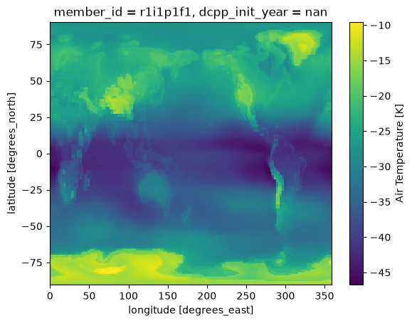
The full temperature feedback is the sum of these, normalized by the change in GMST:
t_feedback = (dLW_ta + dLW_ts)/dgmstt_feedback.mean(dim='month').plot(cbar_kwargs={'label': 'W m$^{-2}$ K$^{-1}$'})Could not determine bucket type for bucket name cmip6: Your default credentials were not found. To set up Application Default Credentials, see https://cloud.google.com/docs/authentication/external/set-up-adc for more information., falling back to GCSFileSystem
Could not determine bucket type for bucket name cmip6: Your default credentials were not found. To set up Application Default Credentials, see https://cloud.google.com/docs/authentication/external/set-up-adc for more information., falling back to GCSFileSystem
Could not determine bucket type for bucket name cmip6: Your default credentials were not found. To set up Application Default Credentials, see https://cloud.google.com/docs/authentication/external/set-up-adc for more information., falling back to GCSFileSystem
Could not determine bucket type for bucket name cmip6: Your default credentials were not found. To set up Application Default Credentials, see https://cloud.google.com/docs/authentication/external/set-up-adc for more information., falling back to GCSFileSystem
Could not determine bucket type for bucket name cmip6: Your default credentials were not found. To set up Application Default Credentials, see https://cloud.google.com/docs/authentication/external/set-up-adc for more information., falling back to GCSFileSystem
Could not determine bucket type for bucket name cmip6: Your default credentials were not found. To set up Application Default Credentials, see https://cloud.google.com/docs/authentication/external/set-up-adc for more information., falling back to GCSFileSystem
Could not determine bucket type for bucket name cmip6: Your default credentials were not found. To set up Application Default Credentials, see https://cloud.google.com/docs/authentication/external/set-up-adc for more information., falling back to GCSFileSystem
Could not determine bucket type for bucket name cmip6: Your default credentials were not found. To set up Application Default Credentials, see https://cloud.google.com/docs/authentication/external/set-up-adc for more information., falling back to GCSFileSystem
Could not determine bucket type for bucket name cmip6: Your default credentials were not found. To set up Application Default Credentials, see https://cloud.google.com/docs/authentication/external/set-up-adc for more information., falling back to GCSFileSystem
Could not determine bucket type for bucket name cmip6: Your default credentials were not found. To set up Application Default Credentials, see https://cloud.google.com/docs/authentication/external/set-up-adc for more information., falling back to GCSFileSystem
Could not determine bucket type for bucket name cmip6: Your default credentials were not found. To set up Application Default Credentials, see https://cloud.google.com/docs/authentication/external/set-up-adc for more information., falling back to GCSFileSystem
Could not determine bucket type for bucket name cmip6: Your default credentials were not found. To set up Application Default Credentials, see https://cloud.google.com/docs/authentication/external/set-up-adc for more information., falling back to GCSFileSystem
Could not determine bucket type for bucket name cmip6: Your default credentials were not found. To set up Application Default Credentials, see https://cloud.google.com/docs/authentication/external/set-up-adc for more information., falling back to GCSFileSystem
Could not determine bucket type for bucket name cmip6: Your default credentials were not found. To set up Application Default Credentials, see https://cloud.google.com/docs/authentication/external/set-up-adc for more information., falling back to GCSFileSystem
Could not determine bucket type for bucket name cmip6: Your default credentials were not found. To set up Application Default Credentials, see https://cloud.google.com/docs/authentication/external/set-up-adc for more information., falling back to GCSFileSystem
Could not determine bucket type for bucket name cmip6: Your default credentials were not found. To set up Application Default Credentials, see https://cloud.google.com/docs/authentication/external/set-up-adc for more information., falling back to GCSFileSystem
Could not determine bucket type for bucket name cmip6: Your default credentials were not found. To set up Application Default Credentials, see https://cloud.google.com/docs/authentication/external/set-up-adc for more information., falling back to GCSFileSystem
Could not determine bucket type for bucket name cmip6: Your default credentials were not found. To set up Application Default Credentials, see https://cloud.google.com/docs/authentication/external/set-up-adc for more information., falling back to GCSFileSystem
Could not determine bucket type for bucket name cmip6: Your default credentials were not found. To set up Application Default Credentials, see https://cloud.google.com/docs/authentication/external/set-up-adc for more information., falling back to GCSFileSystem
Could not determine bucket type for bucket name cmip6: Your default credentials were not found. To set up Application Default Credentials, see https://cloud.google.com/docs/authentication/external/set-up-adc for more information., falling back to GCSFileSystem
Could not determine bucket type for bucket name cmip6: Your default credentials were not found. To set up Application Default Credentials, see https://cloud.google.com/docs/authentication/external/set-up-adc for more information., falling back to GCSFileSystem
Could not determine bucket type for bucket name cmip6: Your default credentials were not found. To set up Application Default Credentials, see https://cloud.google.com/docs/authentication/external/set-up-adc for more information., falling back to GCSFileSystem
Could not determine bucket type for bucket name cmip6: Your default credentials were not found. To set up Application Default Credentials, see https://cloud.google.com/docs/authentication/external/set-up-adc for more information., falling back to GCSFileSystem
Could not determine bucket type for bucket name cmip6: Your default credentials were not found. To set up Application Default Credentials, see https://cloud.google.com/docs/authentication/external/set-up-adc for more information., falling back to GCSFileSystem
Could not determine bucket type for bucket name cmip6: Your default credentials were not found. To set up Application Default Credentials, see https://cloud.google.com/docs/authentication/external/set-up-adc for more information., falling back to GCSFileSystem
Could not determine bucket type for bucket name cmip6: Your default credentials were not found. To set up Application Default Credentials, see https://cloud.google.com/docs/authentication/external/set-up-adc for more information., falling back to GCSFileSystem
Could not determine bucket type for bucket name cmip6: Your default credentials were not found. To set up Application Default Credentials, see https://cloud.google.com/docs/authentication/external/set-up-adc for more information., falling back to GCSFileSystem
Could not determine bucket type for bucket name cmip6: Your default credentials were not found. To set up Application Default Credentials, see https://cloud.google.com/docs/authentication/external/set-up-adc for more information., falling back to GCSFileSystem
Could not determine bucket type for bucket name cmip6: Your default credentials were not found. To set up Application Default Credentials, see https://cloud.google.com/docs/authentication/external/set-up-adc for more information., falling back to GCSFileSystem
Could not determine bucket type for bucket name cmip6: Your default credentials were not found. To set up Application Default Credentials, see https://cloud.google.com/docs/authentication/external/set-up-adc for more information., falling back to GCSFileSystem
Could not determine bucket type for bucket name cmip6: Your default credentials were not found. To set up Application Default Credentials, see https://cloud.google.com/docs/authentication/external/set-up-adc for more information., falling back to GCSFileSystem
Could not determine bucket type for bucket name cmip6: Your default credentials were not found. To set up Application Default Credentials, see https://cloud.google.com/docs/authentication/external/set-up-adc for more information., falling back to GCSFileSystem
Could not determine bucket type for bucket name cmip6: Your default credentials were not found. To set up Application Default Credentials, see https://cloud.google.com/docs/authentication/external/set-up-adc for more information., falling back to GCSFileSystem
Could not determine bucket type for bucket name cmip6: Your default credentials were not found. To set up Application Default Credentials, see https://cloud.google.com/docs/authentication/external/set-up-adc for more information., falling back to GCSFileSystem
Could not determine bucket type for bucket name cmip6: Your default credentials were not found. To set up Application Default Credentials, see https://cloud.google.com/docs/authentication/external/set-up-adc for more information., falling back to GCSFileSystem
Could not determine bucket type for bucket name cmip6: Your default credentials were not found. To set up Application Default Credentials, see https://cloud.google.com/docs/authentication/external/set-up-adc for more information., falling back to GCSFileSystem
Could not determine bucket type for bucket name cmip6: Your default credentials were not found. To set up Application Default Credentials, see https://cloud.google.com/docs/authentication/external/set-up-adc for more information., falling back to GCSFileSystem
Could not determine bucket type for bucket name cmip6: Your default credentials were not found. To set up Application Default Credentials, see https://cloud.google.com/docs/authentication/external/set-up-adc for more information., falling back to GCSFileSystem
Could not determine bucket type for bucket name cmip6: Your default credentials were not found. To set up Application Default Credentials, see https://cloud.google.com/docs/authentication/external/set-up-adc for more information., falling back to GCSFileSystem
Could not determine bucket type for bucket name cmip6: Your default credentials were not found. To set up Application Default Credentials, see https://cloud.google.com/docs/authentication/external/set-up-adc for more information., falling back to GCSFileSystem
Could not determine bucket type for bucket name cmip6: Your default credentials were not found. To set up Application Default Credentials, see https://cloud.google.com/docs/authentication/external/set-up-adc for more information., falling back to GCSFileSystem
Could not determine bucket type for bucket name cmip6: Your default credentials were not found. To set up Application Default Credentials, see https://cloud.google.com/docs/authentication/external/set-up-adc for more information., falling back to GCSFileSystem
Could not determine bucket type for bucket name cmip6: Your default credentials were not found. To set up Application Default Credentials, see https://cloud.google.com/docs/authentication/external/set-up-adc for more information., falling back to GCSFileSystem
Could not determine bucket type for bucket name cmip6: Your default credentials were not found. To set up Application Default Credentials, see https://cloud.google.com/docs/authentication/external/set-up-adc for more information., falling back to GCSFileSystem
Could not determine bucket type for bucket name cmip6: Your default credentials were not found. To set up Application Default Credentials, see https://cloud.google.com/docs/authentication/external/set-up-adc for more information., falling back to GCSFileSystem
Could not determine bucket type for bucket name cmip6: Your default credentials were not found. To set up Application Default Credentials, see https://cloud.google.com/docs/authentication/external/set-up-adc for more information., falling back to GCSFileSystem
Could not determine bucket type for bucket name cmip6: Your default credentials were not found. To set up Application Default Credentials, see https://cloud.google.com/docs/authentication/external/set-up-adc for more information., falling back to GCSFileSystem
Could not determine bucket type for bucket name cmip6: Your default credentials were not found. To set up Application Default Credentials, see https://cloud.google.com/docs/authentication/external/set-up-adc for more information., falling back to GCSFileSystem
Could not determine bucket type for bucket name cmip6: Your default credentials were not found. To set up Application Default Credentials, see https://cloud.google.com/docs/authentication/external/set-up-adc for more information., falling back to GCSFileSystem
Could not determine bucket type for bucket name cmip6: Your default credentials were not found. To set up Application Default Credentials, see https://cloud.google.com/docs/authentication/external/set-up-adc for more information., falling back to GCSFileSystem
Could not determine bucket type for bucket name cmip6: Your default credentials were not found. To set up Application Default Credentials, see https://cloud.google.com/docs/authentication/external/set-up-adc for more information., falling back to GCSFileSystem
Could not determine bucket type for bucket name cmip6: Your default credentials were not found. To set up Application Default Credentials, see https://cloud.google.com/docs/authentication/external/set-up-adc for more information., falling back to GCSFileSystem
Could not determine bucket type for bucket name cmip6: Your default credentials were not found. To set up Application Default Credentials, see https://cloud.google.com/docs/authentication/external/set-up-adc for more information., falling back to GCSFileSystem
Could not determine bucket type for bucket name cmip6: Your default credentials were not found. To set up Application Default Credentials, see https://cloud.google.com/docs/authentication/external/set-up-adc for more information., falling back to GCSFileSystem
Could not determine bucket type for bucket name cmip6: Your default credentials were not found. To set up Application Default Credentials, see https://cloud.google.com/docs/authentication/external/set-up-adc for more information., falling back to GCSFileSystem
Could not determine bucket type for bucket name cmip6: Your default credentials were not found. To set up Application Default Credentials, see https://cloud.google.com/docs/authentication/external/set-up-adc for more information., falling back to GCSFileSystem
Could not determine bucket type for bucket name cmip6: Your default credentials were not found. To set up Application Default Credentials, see https://cloud.google.com/docs/authentication/external/set-up-adc for more information., falling back to GCSFileSystem
Could not determine bucket type for bucket name cmip6: Your default credentials were not found. To set up Application Default Credentials, see https://cloud.google.com/docs/authentication/external/set-up-adc for more information., falling back to GCSFileSystem
Could not determine bucket type for bucket name cmip6: Your default credentials were not found. To set up Application Default Credentials, see https://cloud.google.com/docs/authentication/external/set-up-adc for more information., falling back to GCSFileSystem
Could not determine bucket type for bucket name cmip6: Your default credentials were not found. To set up Application Default Credentials, see https://cloud.google.com/docs/authentication/external/set-up-adc for more information., falling back to GCSFileSystem
Could not determine bucket type for bucket name cmip6: Your default credentials were not found. To set up Application Default Credentials, see https://cloud.google.com/docs/authentication/external/set-up-adc for more information., falling back to GCSFileSystem
Could not determine bucket type for bucket name cmip6: Your default credentials were not found. To set up Application Default Credentials, see https://cloud.google.com/docs/authentication/external/set-up-adc for more information., falling back to GCSFileSystem
Could not determine bucket type for bucket name cmip6: Your default credentials were not found. To set up Application Default Credentials, see https://cloud.google.com/docs/authentication/external/set-up-adc for more information., falling back to GCSFileSystem
Could not determine bucket type for bucket name cmip6: Your default credentials were not found. To set up Application Default Credentials, see https://cloud.google.com/docs/authentication/external/set-up-adc for more information., falling back to GCSFileSystem
Could not determine bucket type for bucket name cmip6: Your default credentials were not found. To set up Application Default Credentials, see https://cloud.google.com/docs/authentication/external/set-up-adc for more information., falling back to GCSFileSystem
Could not determine bucket type for bucket name cmip6: Your default credentials were not found. To set up Application Default Credentials, see https://cloud.google.com/docs/authentication/external/set-up-adc for more information., falling back to GCSFileSystem
Could not determine bucket type for bucket name cmip6: Your default credentials were not found. To set up Application Default Credentials, see https://cloud.google.com/docs/authentication/external/set-up-adc for more information., falling back to GCSFileSystem
Could not determine bucket type for bucket name cmip6: Your default credentials were not found. To set up Application Default Credentials, see https://cloud.google.com/docs/authentication/external/set-up-adc for more information., falling back to GCSFileSystem
Could not determine bucket type for bucket name cmip6: Your default credentials were not found. To set up Application Default Credentials, see https://cloud.google.com/docs/authentication/external/set-up-adc for more information., falling back to GCSFileSystem
Could not determine bucket type for bucket name cmip6: Your default credentials were not found. To set up Application Default Credentials, see https://cloud.google.com/docs/authentication/external/set-up-adc for more information., falling back to GCSFileSystem
Could not determine bucket type for bucket name cmip6: Your default credentials were not found. To set up Application Default Credentials, see https://cloud.google.com/docs/authentication/external/set-up-adc for more information., falling back to GCSFileSystem
Could not determine bucket type for bucket name cmip6: Your default credentials were not found. To set up Application Default Credentials, see https://cloud.google.com/docs/authentication/external/set-up-adc for more information., falling back to GCSFileSystem
Could not determine bucket type for bucket name cmip6: Your default credentials were not found. To set up Application Default Credentials, see https://cloud.google.com/docs/authentication/external/set-up-adc for more information., falling back to GCSFileSystem
Could not determine bucket type for bucket name cmip6: Your default credentials were not found. To set up Application Default Credentials, see https://cloud.google.com/docs/authentication/external/set-up-adc for more information., falling back to GCSFileSystem
Could not determine bucket type for bucket name cmip6: Your default credentials were not found. To set up Application Default Credentials, see https://cloud.google.com/docs/authentication/external/set-up-adc for more information., falling back to GCSFileSystem
Could not determine bucket type for bucket name cmip6: Your default credentials were not found. To set up Application Default Credentials, see https://cloud.google.com/docs/authentication/external/set-up-adc for more information., falling back to GCSFileSystem
Could not determine bucket type for bucket name cmip6: Your default credentials were not found. To set up Application Default Credentials, see https://cloud.google.com/docs/authentication/external/set-up-adc for more information., falling back to GCSFileSystem
Could not determine bucket type for bucket name cmip6: Your default credentials were not found. To set up Application Default Credentials, see https://cloud.google.com/docs/authentication/external/set-up-adc for more information., falling back to GCSFileSystem
Could not determine bucket type for bucket name cmip6: Your default credentials were not found. To set up Application Default Credentials, see https://cloud.google.com/docs/authentication/external/set-up-adc for more information., falling back to GCSFileSystem
Could not determine bucket type for bucket name cmip6: Your default credentials were not found. To set up Application Default Credentials, see https://cloud.google.com/docs/authentication/external/set-up-adc for more information., falling back to GCSFileSystem
Could not determine bucket type for bucket name cmip6: Your default credentials were not found. To set up Application Default Credentials, see https://cloud.google.com/docs/authentication/external/set-up-adc for more information., falling back to GCSFileSystem
Could not determine bucket type for bucket name cmip6: Your default credentials were not found. To set up Application Default Credentials, see https://cloud.google.com/docs/authentication/external/set-up-adc for more information., falling back to GCSFileSystem
Could not determine bucket type for bucket name cmip6: Your default credentials were not found. To set up Application Default Credentials, see https://cloud.google.com/docs/authentication/external/set-up-adc for more information., falling back to GCSFileSystem
Could not determine bucket type for bucket name cmip6: Your default credentials were not found. To set up Application Default Credentials, see https://cloud.google.com/docs/authentication/external/set-up-adc for more information., falling back to GCSFileSystem
Could not determine bucket type for bucket name cmip6: Your default credentials were not found. To set up Application Default Credentials, see https://cloud.google.com/docs/authentication/external/set-up-adc for more information., falling back to GCSFileSystem
Could not determine bucket type for bucket name cmip6: Your default credentials were not found. To set up Application Default Credentials, see https://cloud.google.com/docs/authentication/external/set-up-adc for more information., falling back to GCSFileSystem
Could not determine bucket type for bucket name cmip6: Your default credentials were not found. To set up Application Default Credentials, see https://cloud.google.com/docs/authentication/external/set-up-adc for more information., falling back to GCSFileSystem
Could not determine bucket type for bucket name cmip6: Your default credentials were not found. To set up Application Default Credentials, see https://cloud.google.com/docs/authentication/external/set-up-adc for more information., falling back to GCSFileSystem
Could not determine bucket type for bucket name cmip6: Your default credentials were not found. To set up Application Default Credentials, see https://cloud.google.com/docs/authentication/external/set-up-adc for more information., falling back to GCSFileSystem
Could not determine bucket type for bucket name cmip6: Your default credentials were not found. To set up Application Default Credentials, see https://cloud.google.com/docs/authentication/external/set-up-adc for more information., falling back to GCSFileSystem
Could not determine bucket type for bucket name cmip6: Your default credentials were not found. To set up Application Default Credentials, see https://cloud.google.com/docs/authentication/external/set-up-adc for more information., falling back to GCSFileSystem
Could not determine bucket type for bucket name cmip6: Your default credentials were not found. To set up Application Default Credentials, see https://cloud.google.com/docs/authentication/external/set-up-adc for more information., falling back to GCSFileSystem
Could not determine bucket type for bucket name cmip6: Your default credentials were not found. To set up Application Default Credentials, see https://cloud.google.com/docs/authentication/external/set-up-adc for more information., falling back to GCSFileSystem
Could not determine bucket type for bucket name cmip6: Your default credentials were not found. To set up Application Default Credentials, see https://cloud.google.com/docs/authentication/external/set-up-adc for more information., falling back to GCSFileSystem
Could not determine bucket type for bucket name cmip6: Your default credentials were not found. To set up Application Default Credentials, see https://cloud.google.com/docs/authentication/external/set-up-adc for more information., falling back to GCSFileSystem
Could not determine bucket type for bucket name cmip6: Your default credentials were not found. To set up Application Default Credentials, see https://cloud.google.com/docs/authentication/external/set-up-adc for more information., falling back to GCSFileSystem
Could not determine bucket type for bucket name cmip6: Your default credentials were not found. To set up Application Default Credentials, see https://cloud.google.com/docs/authentication/external/set-up-adc for more information., falling back to GCSFileSystem
Could not determine bucket type for bucket name cmip6: Your default credentials were not found. To set up Application Default Credentials, see https://cloud.google.com/docs/authentication/external/set-up-adc for more information., falling back to GCSFileSystem
Could not determine bucket type for bucket name cmip6: Your default credentials were not found. To set up Application Default Credentials, see https://cloud.google.com/docs/authentication/external/set-up-adc for more information., falling back to GCSFileSystem
Could not determine bucket type for bucket name cmip6: Your default credentials were not found. To set up Application Default Credentials, see https://cloud.google.com/docs/authentication/external/set-up-adc for more information., falling back to GCSFileSystem
Could not determine bucket type for bucket name cmip6: Your default credentials were not found. To set up Application Default Credentials, see https://cloud.google.com/docs/authentication/external/set-up-adc for more information., falling back to GCSFileSystem
Could not determine bucket type for bucket name cmip6: Your default credentials were not found. To set up Application Default Credentials, see https://cloud.google.com/docs/authentication/external/set-up-adc for more information., falling back to GCSFileSystem
Could not determine bucket type for bucket name cmip6: Your default credentials were not found. To set up Application Default Credentials, see https://cloud.google.com/docs/authentication/external/set-up-adc for more information., falling back to GCSFileSystem
Could not determine bucket type for bucket name cmip6: Your default credentials were not found. To set up Application Default Credentials, see https://cloud.google.com/docs/authentication/external/set-up-adc for more information., falling back to GCSFileSystem
Could not determine bucket type for bucket name cmip6: Your default credentials were not found. To set up Application Default Credentials, see https://cloud.google.com/docs/authentication/external/set-up-adc for more information., falling back to GCSFileSystem
Could not determine bucket type for bucket name cmip6: Your default credentials were not found. To set up Application Default Credentials, see https://cloud.google.com/docs/authentication/external/set-up-adc for more information., falling back to GCSFileSystem
Could not determine bucket type for bucket name cmip6: Your default credentials were not found. To set up Application Default Credentials, see https://cloud.google.com/docs/authentication/external/set-up-adc for more information., falling back to GCSFileSystem
Could not determine bucket type for bucket name cmip6: Your default credentials were not found. To set up Application Default Credentials, see https://cloud.google.com/docs/authentication/external/set-up-adc for more information., falling back to GCSFileSystem
Could not determine bucket type for bucket name cmip6: Your default credentials were not found. To set up Application Default Credentials, see https://cloud.google.com/docs/authentication/external/set-up-adc for more information., falling back to GCSFileSystem
Could not determine bucket type for bucket name cmip6: Your default credentials were not found. To set up Application Default Credentials, see https://cloud.google.com/docs/authentication/external/set-up-adc for more information., falling back to GCSFileSystem
Could not determine bucket type for bucket name cmip6: Your default credentials were not found. To set up Application Default Credentials, see https://cloud.google.com/docs/authentication/external/set-up-adc for more information., falling back to GCSFileSystem
Could not determine bucket type for bucket name cmip6: Your default credentials were not found. To set up Application Default Credentials, see https://cloud.google.com/docs/authentication/external/set-up-adc for more information., falling back to GCSFileSystem
Could not determine bucket type for bucket name cmip6: Your default credentials were not found. To set up Application Default Credentials, see https://cloud.google.com/docs/authentication/external/set-up-adc for more information., falling back to GCSFileSystem
Could not determine bucket type for bucket name cmip6: Your default credentials were not found. To set up Application Default Credentials, see https://cloud.google.com/docs/authentication/external/set-up-adc for more information., falling back to GCSFileSystem
Could not determine bucket type for bucket name cmip6: Your default credentials were not found. To set up Application Default Credentials, see https://cloud.google.com/docs/authentication/external/set-up-adc for more information., falling back to GCSFileSystem
Could not determine bucket type for bucket name cmip6: Your default credentials were not found. To set up Application Default Credentials, see https://cloud.google.com/docs/authentication/external/set-up-adc for more information., falling back to GCSFileSystem
Could not determine bucket type for bucket name cmip6: Your default credentials were not found. To set up Application Default Credentials, see https://cloud.google.com/docs/authentication/external/set-up-adc for more information., falling back to GCSFileSystem
Could not determine bucket type for bucket name cmip6: Your default credentials were not found. To set up Application Default Credentials, see https://cloud.google.com/docs/authentication/external/set-up-adc for more information., falling back to GCSFileSystem
Could not determine bucket type for bucket name cmip6: Your default credentials were not found. To set up Application Default Credentials, see https://cloud.google.com/docs/authentication/external/set-up-adc for more information., falling back to GCSFileSystem
Could not determine bucket type for bucket name cmip6: Your default credentials were not found. To set up Application Default Credentials, see https://cloud.google.com/docs/authentication/external/set-up-adc for more information., falling back to GCSFileSystem
Could not determine bucket type for bucket name cmip6: Your default credentials were not found. To set up Application Default Credentials, see https://cloud.google.com/docs/authentication/external/set-up-adc for more information., falling back to GCSFileSystem
Could not determine bucket type for bucket name cmip6: Your default credentials were not found. To set up Application Default Credentials, see https://cloud.google.com/docs/authentication/external/set-up-adc for more information., falling back to GCSFileSystem
Could not determine bucket type for bucket name cmip6: Your default credentials were not found. To set up Application Default Credentials, see https://cloud.google.com/docs/authentication/external/set-up-adc for more information., falling back to GCSFileSystem
Could not determine bucket type for bucket name cmip6: Your default credentials were not found. To set up Application Default Credentials, see https://cloud.google.com/docs/authentication/external/set-up-adc for more information., falling back to GCSFileSystem
Could not determine bucket type for bucket name cmip6: Your default credentials were not found. To set up Application Default Credentials, see https://cloud.google.com/docs/authentication/external/set-up-adc for more information., falling back to GCSFileSystem
Could not determine bucket type for bucket name cmip6: Your default credentials were not found. To set up Application Default Credentials, see https://cloud.google.com/docs/authentication/external/set-up-adc for more information., falling back to GCSFileSystem
Could not determine bucket type for bucket name cmip6: Your default credentials were not found. To set up Application Default Credentials, see https://cloud.google.com/docs/authentication/external/set-up-adc for more information., falling back to GCSFileSystem
Could not determine bucket type for bucket name cmip6: Your default credentials were not found. To set up Application Default Credentials, see https://cloud.google.com/docs/authentication/external/set-up-adc for more information., falling back to GCSFileSystem
Could not determine bucket type for bucket name cmip6: Your default credentials were not found. To set up Application Default Credentials, see https://cloud.google.com/docs/authentication/external/set-up-adc for more information., falling back to GCSFileSystem
Could not determine bucket type for bucket name cmip6: Your default credentials were not found. To set up Application Default Credentials, see https://cloud.google.com/docs/authentication/external/set-up-adc for more information., falling back to GCSFileSystem
Could not determine bucket type for bucket name cmip6: Your default credentials were not found. To set up Application Default Credentials, see https://cloud.google.com/docs/authentication/external/set-up-adc for more information., falling back to GCSFileSystem
Could not determine bucket type for bucket name cmip6: Your default credentials were not found. To set up Application Default Credentials, see https://cloud.google.com/docs/authentication/external/set-up-adc for more information., falling back to GCSFileSystem
Could not determine bucket type for bucket name cmip6: Your default credentials were not found. To set up Application Default Credentials, see https://cloud.google.com/docs/authentication/external/set-up-adc for more information., falling back to GCSFileSystem
Could not determine bucket type for bucket name cmip6: Your default credentials were not found. To set up Application Default Credentials, see https://cloud.google.com/docs/authentication/external/set-up-adc for more information., falling back to GCSFileSystem
Could not determine bucket type for bucket name cmip6: Your default credentials were not found. To set up Application Default Credentials, see https://cloud.google.com/docs/authentication/external/set-up-adc for more information., falling back to GCSFileSystem
Could not determine bucket type for bucket name cmip6: Your default credentials were not found. To set up Application Default Credentials, see https://cloud.google.com/docs/authentication/external/set-up-adc for more information., falling back to GCSFileSystem
Could not determine bucket type for bucket name cmip6: Your default credentials were not found. To set up Application Default Credentials, see https://cloud.google.com/docs/authentication/external/set-up-adc for more information., falling back to GCSFileSystem
Could not determine bucket type for bucket name cmip6: Your default credentials were not found. To set up Application Default Credentials, see https://cloud.google.com/docs/authentication/external/set-up-adc for more information., falling back to GCSFileSystem
Could not determine bucket type for bucket name cmip6: Your default credentials were not found. To set up Application Default Credentials, see https://cloud.google.com/docs/authentication/external/set-up-adc for more information., falling back to GCSFileSystem
Could not determine bucket type for bucket name cmip6: Your default credentials were not found. To set up Application Default Credentials, see https://cloud.google.com/docs/authentication/external/set-up-adc for more information., falling back to GCSFileSystem
Could not determine bucket type for bucket name cmip6: Your default credentials were not found. To set up Application Default Credentials, see https://cloud.google.com/docs/authentication/external/set-up-adc for more information., falling back to GCSFileSystem
Could not determine bucket type for bucket name cmip6: Your default credentials were not found. To set up Application Default Credentials, see https://cloud.google.com/docs/authentication/external/set-up-adc for more information., falling back to GCSFileSystem
Could not determine bucket type for bucket name cmip6: Your default credentials were not found. To set up Application Default Credentials, see https://cloud.google.com/docs/authentication/external/set-up-adc for more information., falling back to GCSFileSystem
Could not determine bucket type for bucket name cmip6: Your default credentials were not found. To set up Application Default Credentials, see https://cloud.google.com/docs/authentication/external/set-up-adc for more information., falling back to GCSFileSystem
Could not determine bucket type for bucket name cmip6: Your default credentials were not found. To set up Application Default Credentials, see https://cloud.google.com/docs/authentication/external/set-up-adc for more information., falling back to GCSFileSystem
Could not determine bucket type for bucket name cmip6: Your default credentials were not found. To set up Application Default Credentials, see https://cloud.google.com/docs/authentication/external/set-up-adc for more information., falling back to GCSFileSystem
Could not determine bucket type for bucket name cmip6: Your default credentials were not found. To set up Application Default Credentials, see https://cloud.google.com/docs/authentication/external/set-up-adc for more information., falling back to GCSFileSystem
Could not determine bucket type for bucket name cmip6: Your default credentials were not found. To set up Application Default Credentials, see https://cloud.google.com/docs/authentication/external/set-up-adc for more information., falling back to GCSFileSystem
Could not determine bucket type for bucket name cmip6: Your default credentials were not found. To set up Application Default Credentials, see https://cloud.google.com/docs/authentication/external/set-up-adc for more information., falling back to GCSFileSystem
Could not determine bucket type for bucket name cmip6: Your default credentials were not found. To set up Application Default Credentials, see https://cloud.google.com/docs/authentication/external/set-up-adc for more information., falling back to GCSFileSystem
Could not determine bucket type for bucket name cmip6: Your default credentials were not found. To set up Application Default Credentials, see https://cloud.google.com/docs/authentication/external/set-up-adc for more information., falling back to GCSFileSystem
Could not determine bucket type for bucket name cmip6: Your default credentials were not found. To set up Application Default Credentials, see https://cloud.google.com/docs/authentication/external/set-up-adc for more information., falling back to GCSFileSystem
Could not determine bucket type for bucket name cmip6: Your default credentials were not found. To set up Application Default Credentials, see https://cloud.google.com/docs/authentication/external/set-up-adc for more information., falling back to GCSFileSystem
Could not determine bucket type for bucket name cmip6: Your default credentials were not found. To set up Application Default Credentials, see https://cloud.google.com/docs/authentication/external/set-up-adc for more information., falling back to GCSFileSystem
Could not determine bucket type for bucket name cmip6: Your default credentials were not found. To set up Application Default Credentials, see https://cloud.google.com/docs/authentication/external/set-up-adc for more information., falling back to GCSFileSystem
Could not determine bucket type for bucket name cmip6: Your default credentials were not found. To set up Application Default Credentials, see https://cloud.google.com/docs/authentication/external/set-up-adc for more information., falling back to GCSFileSystem
Could not determine bucket type for bucket name cmip6: Your default credentials were not found. To set up Application Default Credentials, see https://cloud.google.com/docs/authentication/external/set-up-adc for more information., falling back to GCSFileSystem
Could not determine bucket type for bucket name cmip6: Your default credentials were not found. To set up Application Default Credentials, see https://cloud.google.com/docs/authentication/external/set-up-adc for more information., falling back to GCSFileSystem
Could not determine bucket type for bucket name cmip6: Your default credentials were not found. To set up Application Default Credentials, see https://cloud.google.com/docs/authentication/external/set-up-adc for more information., falling back to GCSFileSystem
Could not determine bucket type for bucket name cmip6: Your default credentials were not found. To set up Application Default Credentials, see https://cloud.google.com/docs/authentication/external/set-up-adc for more information., falling back to GCSFileSystem
Could not determine bucket type for bucket name cmip6: Your default credentials were not found. To set up Application Default Credentials, see https://cloud.google.com/docs/authentication/external/set-up-adc for more information., falling back to GCSFileSystem
Could not determine bucket type for bucket name cmip6: Your default credentials were not found. To set up Application Default Credentials, see https://cloud.google.com/docs/authentication/external/set-up-adc for more information., falling back to GCSFileSystem
Could not determine bucket type for bucket name cmip6: Your default credentials were not found. To set up Application Default Credentials, see https://cloud.google.com/docs/authentication/external/set-up-adc for more information., falling back to GCSFileSystem
Could not determine bucket type for bucket name cmip6: Your default credentials were not found. To set up Application Default Credentials, see https://cloud.google.com/docs/authentication/external/set-up-adc for more information., falling back to GCSFileSystem
Could not determine bucket type for bucket name cmip6: Your default credentials were not found. To set up Application Default Credentials, see https://cloud.google.com/docs/authentication/external/set-up-adc for more information., falling back to GCSFileSystem
Could not determine bucket type for bucket name cmip6: Your default credentials were not found. To set up Application Default Credentials, see https://cloud.google.com/docs/authentication/external/set-up-adc for more information., falling back to GCSFileSystem
Could not determine bucket type for bucket name cmip6: Your default credentials were not found. To set up Application Default Credentials, see https://cloud.google.com/docs/authentication/external/set-up-adc for more information., falling back to GCSFileSystem
Could not determine bucket type for bucket name cmip6: Your default credentials were not found. To set up Application Default Credentials, see https://cloud.google.com/docs/authentication/external/set-up-adc for more information., falling back to GCSFileSystem
Could not determine bucket type for bucket name cmip6: Your default credentials were not found. To set up Application Default Credentials, see https://cloud.google.com/docs/authentication/external/set-up-adc for more information., falling back to GCSFileSystem
Could not determine bucket type for bucket name cmip6: Your default credentials were not found. To set up Application Default Credentials, see https://cloud.google.com/docs/authentication/external/set-up-adc for more information., falling back to GCSFileSystem
Could not determine bucket type for bucket name cmip6: Your default credentials were not found. To set up Application Default Credentials, see https://cloud.google.com/docs/authentication/external/set-up-adc for more information., falling back to GCSFileSystem
Could not determine bucket type for bucket name cmip6: Your default credentials were not found. To set up Application Default Credentials, see https://cloud.google.com/docs/authentication/external/set-up-adc for more information., falling back to GCSFileSystem
Could not determine bucket type for bucket name cmip6: Your default credentials were not found. To set up Application Default Credentials, see https://cloud.google.com/docs/authentication/external/set-up-adc for more information., falling back to GCSFileSystem
Could not determine bucket type for bucket name cmip6: Your default credentials were not found. To set up Application Default Credentials, see https://cloud.google.com/docs/authentication/external/set-up-adc for more information., falling back to GCSFileSystem
Could not determine bucket type for bucket name cmip6: Your default credentials were not found. To set up Application Default Credentials, see https://cloud.google.com/docs/authentication/external/set-up-adc for more information., falling back to GCSFileSystem
Could not determine bucket type for bucket name cmip6: Your default credentials were not found. To set up Application Default Credentials, see https://cloud.google.com/docs/authentication/external/set-up-adc for more information., falling back to GCSFileSystem
Could not determine bucket type for bucket name cmip6: Your default credentials were not found. To set up Application Default Credentials, see https://cloud.google.com/docs/authentication/external/set-up-adc for more information., falling back to GCSFileSystem
Could not determine bucket type for bucket name cmip6: Your default credentials were not found. To set up Application Default Credentials, see https://cloud.google.com/docs/authentication/external/set-up-adc for more information., falling back to GCSFileSystem
Could not determine bucket type for bucket name cmip6: Your default credentials were not found. To set up Application Default Credentials, see https://cloud.google.com/docs/authentication/external/set-up-adc for more information., falling back to GCSFileSystem
Could not determine bucket type for bucket name cmip6: Your default credentials were not found. To set up Application Default Credentials, see https://cloud.google.com/docs/authentication/external/set-up-adc for more information., falling back to GCSFileSystem
Could not determine bucket type for bucket name cmip6: Your default credentials were not found. To set up Application Default Credentials, see https://cloud.google.com/docs/authentication/external/set-up-adc for more information., falling back to GCSFileSystem
Could not determine bucket type for bucket name cmip6: Your default credentials were not found. To set up Application Default Credentials, see https://cloud.google.com/docs/authentication/external/set-up-adc for more information., falling back to GCSFileSystem
Could not determine bucket type for bucket name cmip6: Your default credentials were not found. To set up Application Default Credentials, see https://cloud.google.com/docs/authentication/external/set-up-adc for more information., falling back to GCSFileSystem
Could not determine bucket type for bucket name cmip6: Your default credentials were not found. To set up Application Default Credentials, see https://cloud.google.com/docs/authentication/external/set-up-adc for more information., falling back to GCSFileSystem
Could not determine bucket type for bucket name cmip6: Your default credentials were not found. To set up Application Default Credentials, see https://cloud.google.com/docs/authentication/external/set-up-adc for more information., falling back to GCSFileSystem
Could not determine bucket type for bucket name cmip6: Your default credentials were not found. To set up Application Default Credentials, see https://cloud.google.com/docs/authentication/external/set-up-adc for more information., falling back to GCSFileSystem
Could not determine bucket type for bucket name cmip6: Your default credentials were not found. To set up Application Default Credentials, see https://cloud.google.com/docs/authentication/external/set-up-adc for more information., falling back to GCSFileSystem
Could not determine bucket type for bucket name cmip6: Your default credentials were not found. To set up Application Default Credentials, see https://cloud.google.com/docs/authentication/external/set-up-adc for more information., falling back to GCSFileSystem
Could not determine bucket type for bucket name cmip6: Your default credentials were not found. To set up Application Default Credentials, see https://cloud.google.com/docs/authentication/external/set-up-adc for more information., falling back to GCSFileSystem
Could not determine bucket type for bucket name cmip6: Your default credentials were not found. To set up Application Default Credentials, see https://cloud.google.com/docs/authentication/external/set-up-adc for more information., falling back to GCSFileSystem
Could not determine bucket type for bucket name cmip6: Your default credentials were not found. To set up Application Default Credentials, see https://cloud.google.com/docs/authentication/external/set-up-adc for more information., falling back to GCSFileSystem
Could not determine bucket type for bucket name cmip6: Your default credentials were not found. To set up Application Default Credentials, see https://cloud.google.com/docs/authentication/external/set-up-adc for more information., falling back to GCSFileSystem
Could not determine bucket type for bucket name cmip6: Your default credentials were not found. To set up Application Default Credentials, see https://cloud.google.com/docs/authentication/external/set-up-adc for more information., falling back to GCSFileSystem
Could not determine bucket type for bucket name cmip6: Your default credentials were not found. To set up Application Default Credentials, see https://cloud.google.com/docs/authentication/external/set-up-adc for more information., falling back to GCSFileSystem
Could not determine bucket type for bucket name cmip6: Your default credentials were not found. To set up Application Default Credentials, see https://cloud.google.com/docs/authentication/external/set-up-adc for more information., falling back to GCSFileSystem
Could not determine bucket type for bucket name cmip6: Your default credentials were not found. To set up Application Default Credentials, see https://cloud.google.com/docs/authentication/external/set-up-adc for more information., falling back to GCSFileSystem
Could not determine bucket type for bucket name cmip6: Your default credentials were not found. To set up Application Default Credentials, see https://cloud.google.com/docs/authentication/external/set-up-adc for more information., falling back to GCSFileSystem
Could not determine bucket type for bucket name cmip6: Your default credentials were not found. To set up Application Default Credentials, see https://cloud.google.com/docs/authentication/external/set-up-adc for more information., falling back to GCSFileSystem
Could not determine bucket type for bucket name cmip6: Your default credentials were not found. To set up Application Default Credentials, see https://cloud.google.com/docs/authentication/external/set-up-adc for more information., falling back to GCSFileSystem
Could not determine bucket type for bucket name cmip6: Your default credentials were not found. To set up Application Default Credentials, see https://cloud.google.com/docs/authentication/external/set-up-adc for more information., falling back to GCSFileSystem
Could not determine bucket type for bucket name cmip6: Your default credentials were not found. To set up Application Default Credentials, see https://cloud.google.com/docs/authentication/external/set-up-adc for more information., falling back to GCSFileSystem
Could not determine bucket type for bucket name cmip6: Your default credentials were not found. To set up Application Default Credentials, see https://cloud.google.com/docs/authentication/external/set-up-adc for more information., falling back to GCSFileSystem
Could not determine bucket type for bucket name cmip6: Your default credentials were not found. To set up Application Default Credentials, see https://cloud.google.com/docs/authentication/external/set-up-adc for more information., falling back to GCSFileSystem
Could not determine bucket type for bucket name cmip6: Your default credentials were not found. To set up Application Default Credentials, see https://cloud.google.com/docs/authentication/external/set-up-adc for more information., falling back to GCSFileSystem
Could not determine bucket type for bucket name cmip6: Your default credentials were not found. To set up Application Default Credentials, see https://cloud.google.com/docs/authentication/external/set-up-adc for more information., falling back to GCSFileSystem
Could not determine bucket type for bucket name cmip6: Your default credentials were not found. To set up Application Default Credentials, see https://cloud.google.com/docs/authentication/external/set-up-adc for more information., falling back to GCSFileSystem
Could not determine bucket type for bucket name cmip6: Your default credentials were not found. To set up Application Default Credentials, see https://cloud.google.com/docs/authentication/external/set-up-adc for more information., falling back to GCSFileSystem
Could not determine bucket type for bucket name cmip6: Your default credentials were not found. To set up Application Default Credentials, see https://cloud.google.com/docs/authentication/external/set-up-adc for more information., falling back to GCSFileSystem
Could not determine bucket type for bucket name cmip6: Your default credentials were not found. To set up Application Default Credentials, see https://cloud.google.com/docs/authentication/external/set-up-adc for more information., falling back to GCSFileSystem
Could not determine bucket type for bucket name cmip6: Your default credentials were not found. To set up Application Default Credentials, see https://cloud.google.com/docs/authentication/external/set-up-adc for more information., falling back to GCSFileSystem
Could not determine bucket type for bucket name cmip6: Your default credentials were not found. To set up Application Default Credentials, see https://cloud.google.com/docs/authentication/external/set-up-adc for more information., falling back to GCSFileSystem
Could not determine bucket type for bucket name cmip6: Your default credentials were not found. To set up Application Default Credentials, see https://cloud.google.com/docs/authentication/external/set-up-adc for more information., falling back to GCSFileSystem
Could not determine bucket type for bucket name cmip6: Your default credentials were not found. To set up Application Default Credentials, see https://cloud.google.com/docs/authentication/external/set-up-adc for more information., falling back to GCSFileSystem
Could not determine bucket type for bucket name cmip6: Your default credentials were not found. To set up Application Default Credentials, see https://cloud.google.com/docs/authentication/external/set-up-adc for more information., falling back to GCSFileSystem
Could not determine bucket type for bucket name cmip6: Your default credentials were not found. To set up Application Default Credentials, see https://cloud.google.com/docs/authentication/external/set-up-adc for more information., falling back to GCSFileSystem
Could not determine bucket type for bucket name cmip6: Your default credentials were not found. To set up Application Default Credentials, see https://cloud.google.com/docs/authentication/external/set-up-adc for more information., falling back to GCSFileSystem
Could not determine bucket type for bucket name cmip6: Your default credentials were not found. To set up Application Default Credentials, see https://cloud.google.com/docs/authentication/external/set-up-adc for more information., falling back to GCSFileSystem
Could not determine bucket type for bucket name cmip6: Your default credentials were not found. To set up Application Default Credentials, see https://cloud.google.com/docs/authentication/external/set-up-adc for more information., falling back to GCSFileSystem
Could not determine bucket type for bucket name cmip6: Your default credentials were not found. To set up Application Default Credentials, see https://cloud.google.com/docs/authentication/external/set-up-adc for more information., falling back to GCSFileSystem
Could not determine bucket type for bucket name cmip6: Your default credentials were not found. To set up Application Default Credentials, see https://cloud.google.com/docs/authentication/external/set-up-adc for more information., falling back to GCSFileSystem
Could not determine bucket type for bucket name cmip6: Your default credentials were not found. To set up Application Default Credentials, see https://cloud.google.com/docs/authentication/external/set-up-adc for more information., falling back to GCSFileSystem
Could not determine bucket type for bucket name cmip6: Your default credentials were not found. To set up Application Default Credentials, see https://cloud.google.com/docs/authentication/external/set-up-adc for more information., falling back to GCSFileSystem
Could not determine bucket type for bucket name cmip6: Your default credentials were not found. To set up Application Default Credentials, see https://cloud.google.com/docs/authentication/external/set-up-adc for more information., falling back to GCSFileSystem
Could not determine bucket type for bucket name cmip6: Your default credentials were not found. To set up Application Default Credentials, see https://cloud.google.com/docs/authentication/external/set-up-adc for more information., falling back to GCSFileSystem
Could not determine bucket type for bucket name cmip6: Your default credentials were not found. To set up Application Default Credentials, see https://cloud.google.com/docs/authentication/external/set-up-adc for more information., falling back to GCSFileSystem
Could not determine bucket type for bucket name cmip6: Your default credentials were not found. To set up Application Default Credentials, see https://cloud.google.com/docs/authentication/external/set-up-adc for more information., falling back to GCSFileSystem
Could not determine bucket type for bucket name cmip6: Your default credentials were not found. To set up Application Default Credentials, see https://cloud.google.com/docs/authentication/external/set-up-adc for more information., falling back to GCSFileSystem
Could not determine bucket type for bucket name cmip6: Your default credentials were not found. To set up Application Default Credentials, see https://cloud.google.com/docs/authentication/external/set-up-adc for more information., falling back to GCSFileSystem
Could not determine bucket type for bucket name cmip6: Your default credentials were not found. To set up Application Default Credentials, see https://cloud.google.com/docs/authentication/external/set-up-adc for more information., falling back to GCSFileSystem
Could not determine bucket type for bucket name cmip6: Your default credentials were not found. To set up Application Default Credentials, see https://cloud.google.com/docs/authentication/external/set-up-adc for more information., falling back to GCSFileSystem
Could not determine bucket type for bucket name cmip6: Your default credentials were not found. To set up Application Default Credentials, see https://cloud.google.com/docs/authentication/external/set-up-adc for more information., falling back to GCSFileSystem
Could not determine bucket type for bucket name cmip6: Your default credentials were not found. To set up Application Default Credentials, see https://cloud.google.com/docs/authentication/external/set-up-adc for more information., falling back to GCSFileSystem
Could not determine bucket type for bucket name cmip6: Your default credentials were not found. To set up Application Default Credentials, see https://cloud.google.com/docs/authentication/external/set-up-adc for more information., falling back to GCSFileSystem
Could not determine bucket type for bucket name cmip6: Your default credentials were not found. To set up Application Default Credentials, see https://cloud.google.com/docs/authentication/external/set-up-adc for more information., falling back to GCSFileSystem
Could not determine bucket type for bucket name cmip6: Your default credentials were not found. To set up Application Default Credentials, see https://cloud.google.com/docs/authentication/external/set-up-adc for more information., falling back to GCSFileSystem
Could not determine bucket type for bucket name cmip6: Your default credentials were not found. To set up Application Default Credentials, see https://cloud.google.com/docs/authentication/external/set-up-adc for more information., falling back to GCSFileSystem
Could not determine bucket type for bucket name cmip6: Your default credentials were not found. To set up Application Default Credentials, see https://cloud.google.com/docs/authentication/external/set-up-adc for more information., falling back to GCSFileSystem
Could not determine bucket type for bucket name cmip6: Your default credentials were not found. To set up Application Default Credentials, see https://cloud.google.com/docs/authentication/external/set-up-adc for more information., falling back to GCSFileSystem
Could not determine bucket type for bucket name cmip6: Your default credentials were not found. To set up Application Default Credentials, see https://cloud.google.com/docs/authentication/external/set-up-adc for more information., falling back to GCSFileSystem
Could not determine bucket type for bucket name cmip6: Your default credentials were not found. To set up Application Default Credentials, see https://cloud.google.com/docs/authentication/external/set-up-adc for more information., falling back to GCSFileSystem
Could not determine bucket type for bucket name cmip6: Your default credentials were not found. To set up Application Default Credentials, see https://cloud.google.com/docs/authentication/external/set-up-adc for more information., falling back to GCSFileSystem
Could not determine bucket type for bucket name cmip6: Your default credentials were not found. To set up Application Default Credentials, see https://cloud.google.com/docs/authentication/external/set-up-adc for more information., falling back to GCSFileSystem
Could not determine bucket type for bucket name cmip6: Your default credentials were not found. To set up Application Default Credentials, see https://cloud.google.com/docs/authentication/external/set-up-adc for more information., falling back to GCSFileSystem
Could not determine bucket type for bucket name cmip6: Your default credentials were not found. To set up Application Default Credentials, see https://cloud.google.com/docs/authentication/external/set-up-adc for more information., falling back to GCSFileSystem
Could not determine bucket type for bucket name cmip6: Your default credentials were not found. To set up Application Default Credentials, see https://cloud.google.com/docs/authentication/external/set-up-adc for more information., falling back to GCSFileSystem
Could not determine bucket type for bucket name cmip6: Your default credentials were not found. To set up Application Default Credentials, see https://cloud.google.com/docs/authentication/external/set-up-adc for more information., falling back to GCSFileSystem
Could not determine bucket type for bucket name cmip6: Your default credentials were not found. To set up Application Default Credentials, see https://cloud.google.com/docs/authentication/external/set-up-adc for more information., falling back to GCSFileSystem
Could not determine bucket type for bucket name cmip6: Your default credentials were not found. To set up Application Default Credentials, see https://cloud.google.com/docs/authentication/external/set-up-adc for more information., falling back to GCSFileSystem
Could not determine bucket type for bucket name cmip6: Your default credentials were not found. To set up Application Default Credentials, see https://cloud.google.com/docs/authentication/external/set-up-adc for more information., falling back to GCSFileSystem
Could not determine bucket type for bucket name cmip6: Your default credentials were not found. To set up Application Default Credentials, see https://cloud.google.com/docs/authentication/external/set-up-adc for more information., falling back to GCSFileSystem
Could not determine bucket type for bucket name cmip6: Your default credentials were not found. To set up Application Default Credentials, see https://cloud.google.com/docs/authentication/external/set-up-adc for more information., falling back to GCSFileSystem
Could not determine bucket type for bucket name cmip6: Your default credentials were not found. To set up Application Default Credentials, see https://cloud.google.com/docs/authentication/external/set-up-adc for more information., falling back to GCSFileSystem
Could not determine bucket type for bucket name cmip6: Your default credentials were not found. To set up Application Default Credentials, see https://cloud.google.com/docs/authentication/external/set-up-adc for more information., falling back to GCSFileSystem
Could not determine bucket type for bucket name cmip6: Your default credentials were not found. To set up Application Default Credentials, see https://cloud.google.com/docs/authentication/external/set-up-adc for more information., falling back to GCSFileSystem
Could not determine bucket type for bucket name cmip6: Your default credentials were not found. To set up Application Default Credentials, see https://cloud.google.com/docs/authentication/external/set-up-adc for more information., falling back to GCSFileSystem
Could not determine bucket type for bucket name cmip6: Your default credentials were not found. To set up Application Default Credentials, see https://cloud.google.com/docs/authentication/external/set-up-adc for more information., falling back to GCSFileSystem
Could not determine bucket type for bucket name cmip6: Your default credentials were not found. To set up Application Default Credentials, see https://cloud.google.com/docs/authentication/external/set-up-adc for more information., falling back to GCSFileSystem
Could not determine bucket type for bucket name cmip6: Your default credentials were not found. To set up Application Default Credentials, see https://cloud.google.com/docs/authentication/external/set-up-adc for more information., falling back to GCSFileSystem
Could not determine bucket type for bucket name cmip6: Your default credentials were not found. To set up Application Default Credentials, see https://cloud.google.com/docs/authentication/external/set-up-adc for more information., falling back to GCSFileSystem
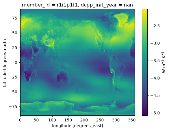
For the annual and global average, we get in W m K:
gm_t_feedback = global_average(t_feedback.mean(dim='month')).load()
gm_t_feedbackCould not determine bucket type for bucket name cmip6: Your default credentials were not found. To set up Application Default Credentials, see https://cloud.google.com/docs/authentication/external/set-up-adc for more information., falling back to GCSFileSystem
Could not determine bucket type for bucket name cmip6: Your default credentials were not found. To set up Application Default Credentials, see https://cloud.google.com/docs/authentication/external/set-up-adc for more information., falling back to GCSFileSystem
Could not determine bucket type for bucket name cmip6: Your default credentials were not found. To set up Application Default Credentials, see https://cloud.google.com/docs/authentication/external/set-up-adc for more information., falling back to GCSFileSystem
Could not determine bucket type for bucket name cmip6: Your default credentials were not found. To set up Application Default Credentials, see https://cloud.google.com/docs/authentication/external/set-up-adc for more information., falling back to GCSFileSystem
Could not determine bucket type for bucket name cmip6: Your default credentials were not found. To set up Application Default Credentials, see https://cloud.google.com/docs/authentication/external/set-up-adc for more information., falling back to GCSFileSystem
Could not determine bucket type for bucket name cmip6: Your default credentials were not found. To set up Application Default Credentials, see https://cloud.google.com/docs/authentication/external/set-up-adc for more information., falling back to GCSFileSystem
Could not determine bucket type for bucket name cmip6: Your default credentials were not found. To set up Application Default Credentials, see https://cloud.google.com/docs/authentication/external/set-up-adc for more information., falling back to GCSFileSystem
Could not determine bucket type for bucket name cmip6: Your default credentials were not found. To set up Application Default Credentials, see https://cloud.google.com/docs/authentication/external/set-up-adc for more information., falling back to GCSFileSystem
Could not determine bucket type for bucket name cmip6: Your default credentials were not found. To set up Application Default Credentials, see https://cloud.google.com/docs/authentication/external/set-up-adc for more information., falling back to GCSFileSystem
Could not determine bucket type for bucket name cmip6: Your default credentials were not found. To set up Application Default Credentials, see https://cloud.google.com/docs/authentication/external/set-up-adc for more information., falling back to GCSFileSystem
Could not determine bucket type for bucket name cmip6: Your default credentials were not found. To set up Application Default Credentials, see https://cloud.google.com/docs/authentication/external/set-up-adc for more information., falling back to GCSFileSystem
Could not determine bucket type for bucket name cmip6: Your default credentials were not found. To set up Application Default Credentials, see https://cloud.google.com/docs/authentication/external/set-up-adc for more information., falling back to GCSFileSystem
Could not determine bucket type for bucket name cmip6: Your default credentials were not found. To set up Application Default Credentials, see https://cloud.google.com/docs/authentication/external/set-up-adc for more information., falling back to GCSFileSystem
Could not determine bucket type for bucket name cmip6: Your default credentials were not found. To set up Application Default Credentials, see https://cloud.google.com/docs/authentication/external/set-up-adc for more information., falling back to GCSFileSystem
Could not determine bucket type for bucket name cmip6: Your default credentials were not found. To set up Application Default Credentials, see https://cloud.google.com/docs/authentication/external/set-up-adc for more information., falling back to GCSFileSystem
Could not determine bucket type for bucket name cmip6: Your default credentials were not found. To set up Application Default Credentials, see https://cloud.google.com/docs/authentication/external/set-up-adc for more information., falling back to GCSFileSystem
Could not determine bucket type for bucket name cmip6: Your default credentials were not found. To set up Application Default Credentials, see https://cloud.google.com/docs/authentication/external/set-up-adc for more information., falling back to GCSFileSystem
Could not determine bucket type for bucket name cmip6: Your default credentials were not found. To set up Application Default Credentials, see https://cloud.google.com/docs/authentication/external/set-up-adc for more information., falling back to GCSFileSystem
Could not determine bucket type for bucket name cmip6: Your default credentials were not found. To set up Application Default Credentials, see https://cloud.google.com/docs/authentication/external/set-up-adc for more information., falling back to GCSFileSystem
Could not determine bucket type for bucket name cmip6: Your default credentials were not found. To set up Application Default Credentials, see https://cloud.google.com/docs/authentication/external/set-up-adc for more information., falling back to GCSFileSystem
Could not determine bucket type for bucket name cmip6: Your default credentials were not found. To set up Application Default Credentials, see https://cloud.google.com/docs/authentication/external/set-up-adc for more information., falling back to GCSFileSystem
Could not determine bucket type for bucket name cmip6: Your default credentials were not found. To set up Application Default Credentials, see https://cloud.google.com/docs/authentication/external/set-up-adc for more information., falling back to GCSFileSystem
Could not determine bucket type for bucket name cmip6: Your default credentials were not found. To set up Application Default Credentials, see https://cloud.google.com/docs/authentication/external/set-up-adc for more information., falling back to GCSFileSystem
Could not determine bucket type for bucket name cmip6: Your default credentials were not found. To set up Application Default Credentials, see https://cloud.google.com/docs/authentication/external/set-up-adc for more information., falling back to GCSFileSystem
Could not determine bucket type for bucket name cmip6: Your default credentials were not found. To set up Application Default Credentials, see https://cloud.google.com/docs/authentication/external/set-up-adc for more information., falling back to GCSFileSystem
Could not determine bucket type for bucket name cmip6: Your default credentials were not found. To set up Application Default Credentials, see https://cloud.google.com/docs/authentication/external/set-up-adc for more information., falling back to GCSFileSystem
Could not determine bucket type for bucket name cmip6: Your default credentials were not found. To set up Application Default Credentials, see https://cloud.google.com/docs/authentication/external/set-up-adc for more information., falling back to GCSFileSystem
Could not determine bucket type for bucket name cmip6: Your default credentials were not found. To set up Application Default Credentials, see https://cloud.google.com/docs/authentication/external/set-up-adc for more information., falling back to GCSFileSystem
Could not determine bucket type for bucket name cmip6: Your default credentials were not found. To set up Application Default Credentials, see https://cloud.google.com/docs/authentication/external/set-up-adc for more information., falling back to GCSFileSystem
Could not determine bucket type for bucket name cmip6: Your default credentials were not found. To set up Application Default Credentials, see https://cloud.google.com/docs/authentication/external/set-up-adc for more information., falling back to GCSFileSystem
Could not determine bucket type for bucket name cmip6: Your default credentials were not found. To set up Application Default Credentials, see https://cloud.google.com/docs/authentication/external/set-up-adc for more information., falling back to GCSFileSystem
Could not determine bucket type for bucket name cmip6: Your default credentials were not found. To set up Application Default Credentials, see https://cloud.google.com/docs/authentication/external/set-up-adc for more information., falling back to GCSFileSystem
Could not determine bucket type for bucket name cmip6: Your default credentials were not found. To set up Application Default Credentials, see https://cloud.google.com/docs/authentication/external/set-up-adc for more information., falling back to GCSFileSystem
Could not determine bucket type for bucket name cmip6: Your default credentials were not found. To set up Application Default Credentials, see https://cloud.google.com/docs/authentication/external/set-up-adc for more information., falling back to GCSFileSystem
Could not determine bucket type for bucket name cmip6: Your default credentials were not found. To set up Application Default Credentials, see https://cloud.google.com/docs/authentication/external/set-up-adc for more information., falling back to GCSFileSystem
Could not determine bucket type for bucket name cmip6: Your default credentials were not found. To set up Application Default Credentials, see https://cloud.google.com/docs/authentication/external/set-up-adc for more information., falling back to GCSFileSystem
Could not determine bucket type for bucket name cmip6: Your default credentials were not found. To set up Application Default Credentials, see https://cloud.google.com/docs/authentication/external/set-up-adc for more information., falling back to GCSFileSystem
Could not determine bucket type for bucket name cmip6: Your default credentials were not found. To set up Application Default Credentials, see https://cloud.google.com/docs/authentication/external/set-up-adc for more information., falling back to GCSFileSystem
Could not determine bucket type for bucket name cmip6: Your default credentials were not found. To set up Application Default Credentials, see https://cloud.google.com/docs/authentication/external/set-up-adc for more information., falling back to GCSFileSystem
Could not determine bucket type for bucket name cmip6: Your default credentials were not found. To set up Application Default Credentials, see https://cloud.google.com/docs/authentication/external/set-up-adc for more information., falling back to GCSFileSystem
Could not determine bucket type for bucket name cmip6: Your default credentials were not found. To set up Application Default Credentials, see https://cloud.google.com/docs/authentication/external/set-up-adc for more information., falling back to GCSFileSystem
Could not determine bucket type for bucket name cmip6: Your default credentials were not found. To set up Application Default Credentials, see https://cloud.google.com/docs/authentication/external/set-up-adc for more information., falling back to GCSFileSystem
Could not determine bucket type for bucket name cmip6: Your default credentials were not found. To set up Application Default Credentials, see https://cloud.google.com/docs/authentication/external/set-up-adc for more information., falling back to GCSFileSystem
Could not determine bucket type for bucket name cmip6: Your default credentials were not found. To set up Application Default Credentials, see https://cloud.google.com/docs/authentication/external/set-up-adc for more information., falling back to GCSFileSystem
Could not determine bucket type for bucket name cmip6: Your default credentials were not found. To set up Application Default Credentials, see https://cloud.google.com/docs/authentication/external/set-up-adc for more information., falling back to GCSFileSystem
Could not determine bucket type for bucket name cmip6: Your default credentials were not found. To set up Application Default Credentials, see https://cloud.google.com/docs/authentication/external/set-up-adc for more information., falling back to GCSFileSystem
Could not determine bucket type for bucket name cmip6: Your default credentials were not found. To set up Application Default Credentials, see https://cloud.google.com/docs/authentication/external/set-up-adc for more information., falling back to GCSFileSystem
Could not determine bucket type for bucket name cmip6: Your default credentials were not found. To set up Application Default Credentials, see https://cloud.google.com/docs/authentication/external/set-up-adc for more information., falling back to GCSFileSystem
Could not determine bucket type for bucket name cmip6: Your default credentials were not found. To set up Application Default Credentials, see https://cloud.google.com/docs/authentication/external/set-up-adc for more information., falling back to GCSFileSystem
Could not determine bucket type for bucket name cmip6: Your default credentials were not found. To set up Application Default Credentials, see https://cloud.google.com/docs/authentication/external/set-up-adc for more information., falling back to GCSFileSystem
Could not determine bucket type for bucket name cmip6: Your default credentials were not found. To set up Application Default Credentials, see https://cloud.google.com/docs/authentication/external/set-up-adc for more information., falling back to GCSFileSystem
Could not determine bucket type for bucket name cmip6: Your default credentials were not found. To set up Application Default Credentials, see https://cloud.google.com/docs/authentication/external/set-up-adc for more information., falling back to GCSFileSystem
Could not determine bucket type for bucket name cmip6: Your default credentials were not found. To set up Application Default Credentials, see https://cloud.google.com/docs/authentication/external/set-up-adc for more information., falling back to GCSFileSystem
Could not determine bucket type for bucket name cmip6: Your default credentials were not found. To set up Application Default Credentials, see https://cloud.google.com/docs/authentication/external/set-up-adc for more information., falling back to GCSFileSystem
Could not determine bucket type for bucket name cmip6: Your default credentials were not found. To set up Application Default Credentials, see https://cloud.google.com/docs/authentication/external/set-up-adc for more information., falling back to GCSFileSystem
Could not determine bucket type for bucket name cmip6: Your default credentials were not found. To set up Application Default Credentials, see https://cloud.google.com/docs/authentication/external/set-up-adc for more information., falling back to GCSFileSystem
Could not determine bucket type for bucket name cmip6: Your default credentials were not found. To set up Application Default Credentials, see https://cloud.google.com/docs/authentication/external/set-up-adc for more information., falling back to GCSFileSystem
Could not determine bucket type for bucket name cmip6: Your default credentials were not found. To set up Application Default Credentials, see https://cloud.google.com/docs/authentication/external/set-up-adc for more information., falling back to GCSFileSystem
Could not determine bucket type for bucket name cmip6: Your default credentials were not found. To set up Application Default Credentials, see https://cloud.google.com/docs/authentication/external/set-up-adc for more information., falling back to GCSFileSystem
Could not determine bucket type for bucket name cmip6: Your default credentials were not found. To set up Application Default Credentials, see https://cloud.google.com/docs/authentication/external/set-up-adc for more information., falling back to GCSFileSystem
Could not determine bucket type for bucket name cmip6: Your default credentials were not found. To set up Application Default Credentials, see https://cloud.google.com/docs/authentication/external/set-up-adc for more information., falling back to GCSFileSystem
Could not determine bucket type for bucket name cmip6: Your default credentials were not found. To set up Application Default Credentials, see https://cloud.google.com/docs/authentication/external/set-up-adc for more information., falling back to GCSFileSystem
Could not determine bucket type for bucket name cmip6: Your default credentials were not found. To set up Application Default Credentials, see https://cloud.google.com/docs/authentication/external/set-up-adc for more information., falling back to GCSFileSystem
Could not determine bucket type for bucket name cmip6: Your default credentials were not found. To set up Application Default Credentials, see https://cloud.google.com/docs/authentication/external/set-up-adc for more information., falling back to GCSFileSystem
Could not determine bucket type for bucket name cmip6: Your default credentials were not found. To set up Application Default Credentials, see https://cloud.google.com/docs/authentication/external/set-up-adc for more information., falling back to GCSFileSystem
Could not determine bucket type for bucket name cmip6: Your default credentials were not found. To set up Application Default Credentials, see https://cloud.google.com/docs/authentication/external/set-up-adc for more information., falling back to GCSFileSystem
Could not determine bucket type for bucket name cmip6: Your default credentials were not found. To set up Application Default Credentials, see https://cloud.google.com/docs/authentication/external/set-up-adc for more information., falling back to GCSFileSystem
Could not determine bucket type for bucket name cmip6: Your default credentials were not found. To set up Application Default Credentials, see https://cloud.google.com/docs/authentication/external/set-up-adc for more information., falling back to GCSFileSystem
Could not determine bucket type for bucket name cmip6: Your default credentials were not found. To set up Application Default Credentials, see https://cloud.google.com/docs/authentication/external/set-up-adc for more information., falling back to GCSFileSystem
Could not determine bucket type for bucket name cmip6: Your default credentials were not found. To set up Application Default Credentials, see https://cloud.google.com/docs/authentication/external/set-up-adc for more information., falling back to GCSFileSystem
Could not determine bucket type for bucket name cmip6: Your default credentials were not found. To set up Application Default Credentials, see https://cloud.google.com/docs/authentication/external/set-up-adc for more information., falling back to GCSFileSystem
Could not determine bucket type for bucket name cmip6: Your default credentials were not found. To set up Application Default Credentials, see https://cloud.google.com/docs/authentication/external/set-up-adc for more information., falling back to GCSFileSystem
Could not determine bucket type for bucket name cmip6: Your default credentials were not found. To set up Application Default Credentials, see https://cloud.google.com/docs/authentication/external/set-up-adc for more information., falling back to GCSFileSystem
Could not determine bucket type for bucket name cmip6: Your default credentials were not found. To set up Application Default Credentials, see https://cloud.google.com/docs/authentication/external/set-up-adc for more information., falling back to GCSFileSystem
Could not determine bucket type for bucket name cmip6: Your default credentials were not found. To set up Application Default Credentials, see https://cloud.google.com/docs/authentication/external/set-up-adc for more information., falling back to GCSFileSystem
Could not determine bucket type for bucket name cmip6: Your default credentials were not found. To set up Application Default Credentials, see https://cloud.google.com/docs/authentication/external/set-up-adc for more information., falling back to GCSFileSystem
Could not determine bucket type for bucket name cmip6: Your default credentials were not found. To set up Application Default Credentials, see https://cloud.google.com/docs/authentication/external/set-up-adc for more information., falling back to GCSFileSystem
Could not determine bucket type for bucket name cmip6: Your default credentials were not found. To set up Application Default Credentials, see https://cloud.google.com/docs/authentication/external/set-up-adc for more information., falling back to GCSFileSystem
Could not determine bucket type for bucket name cmip6: Your default credentials were not found. To set up Application Default Credentials, see https://cloud.google.com/docs/authentication/external/set-up-adc for more information., falling back to GCSFileSystem
Could not determine bucket type for bucket name cmip6: Your default credentials were not found. To set up Application Default Credentials, see https://cloud.google.com/docs/authentication/external/set-up-adc for more information., falling back to GCSFileSystem
Could not determine bucket type for bucket name cmip6: Your default credentials were not found. To set up Application Default Credentials, see https://cloud.google.com/docs/authentication/external/set-up-adc for more information., falling back to GCSFileSystem
Could not determine bucket type for bucket name cmip6: Your default credentials were not found. To set up Application Default Credentials, see https://cloud.google.com/docs/authentication/external/set-up-adc for more information., falling back to GCSFileSystem
Could not determine bucket type for bucket name cmip6: Your default credentials were not found. To set up Application Default Credentials, see https://cloud.google.com/docs/authentication/external/set-up-adc for more information., falling back to GCSFileSystem
Could not determine bucket type for bucket name cmip6: Your default credentials were not found. To set up Application Default Credentials, see https://cloud.google.com/docs/authentication/external/set-up-adc for more information., falling back to GCSFileSystem
Could not determine bucket type for bucket name cmip6: Your default credentials were not found. To set up Application Default Credentials, see https://cloud.google.com/docs/authentication/external/set-up-adc for more information., falling back to GCSFileSystem
Could not determine bucket type for bucket name cmip6: Your default credentials were not found. To set up Application Default Credentials, see https://cloud.google.com/docs/authentication/external/set-up-adc for more information., falling back to GCSFileSystem
Could not determine bucket type for bucket name cmip6: Your default credentials were not found. To set up Application Default Credentials, see https://cloud.google.com/docs/authentication/external/set-up-adc for more information., falling back to GCSFileSystem
Could not determine bucket type for bucket name cmip6: Your default credentials were not found. To set up Application Default Credentials, see https://cloud.google.com/docs/authentication/external/set-up-adc for more information., falling back to GCSFileSystem
Could not determine bucket type for bucket name cmip6: Your default credentials were not found. To set up Application Default Credentials, see https://cloud.google.com/docs/authentication/external/set-up-adc for more information., falling back to GCSFileSystem
Could not determine bucket type for bucket name cmip6: Your default credentials were not found. To set up Application Default Credentials, see https://cloud.google.com/docs/authentication/external/set-up-adc for more information., falling back to GCSFileSystem
Could not determine bucket type for bucket name cmip6: Your default credentials were not found. To set up Application Default Credentials, see https://cloud.google.com/docs/authentication/external/set-up-adc for more information., falling back to GCSFileSystem
Could not determine bucket type for bucket name cmip6: Your default credentials were not found. To set up Application Default Credentials, see https://cloud.google.com/docs/authentication/external/set-up-adc for more information., falling back to GCSFileSystem
Could not determine bucket type for bucket name cmip6: Your default credentials were not found. To set up Application Default Credentials, see https://cloud.google.com/docs/authentication/external/set-up-adc for more information., falling back to GCSFileSystem
Could not determine bucket type for bucket name cmip6: Your default credentials were not found. To set up Application Default Credentials, see https://cloud.google.com/docs/authentication/external/set-up-adc for more information., falling back to GCSFileSystem
Could not determine bucket type for bucket name cmip6: Your default credentials were not found. To set up Application Default Credentials, see https://cloud.google.com/docs/authentication/external/set-up-adc for more information., falling back to GCSFileSystem
Could not determine bucket type for bucket name cmip6: Your default credentials were not found. To set up Application Default Credentials, see https://cloud.google.com/docs/authentication/external/set-up-adc for more information., falling back to GCSFileSystem
Could not determine bucket type for bucket name cmip6: Your default credentials were not found. To set up Application Default Credentials, see https://cloud.google.com/docs/authentication/external/set-up-adc for more information., falling back to GCSFileSystem
Could not determine bucket type for bucket name cmip6: Your default credentials were not found. To set up Application Default Credentials, see https://cloud.google.com/docs/authentication/external/set-up-adc for more information., falling back to GCSFileSystem
Could not determine bucket type for bucket name cmip6: Your default credentials were not found. To set up Application Default Credentials, see https://cloud.google.com/docs/authentication/external/set-up-adc for more information., falling back to GCSFileSystem
Could not determine bucket type for bucket name cmip6: Your default credentials were not found. To set up Application Default Credentials, see https://cloud.google.com/docs/authentication/external/set-up-adc for more information., falling back to GCSFileSystem
Could not determine bucket type for bucket name cmip6: Your default credentials were not found. To set up Application Default Credentials, see https://cloud.google.com/docs/authentication/external/set-up-adc for more information., falling back to GCSFileSystem
Could not determine bucket type for bucket name cmip6: Your default credentials were not found. To set up Application Default Credentials, see https://cloud.google.com/docs/authentication/external/set-up-adc for more information., falling back to GCSFileSystem
Could not determine bucket type for bucket name cmip6: Your default credentials were not found. To set up Application Default Credentials, see https://cloud.google.com/docs/authentication/external/set-up-adc for more information., falling back to GCSFileSystem
Could not determine bucket type for bucket name cmip6: Your default credentials were not found. To set up Application Default Credentials, see https://cloud.google.com/docs/authentication/external/set-up-adc for more information., falling back to GCSFileSystem
Could not determine bucket type for bucket name cmip6: Your default credentials were not found. To set up Application Default Credentials, see https://cloud.google.com/docs/authentication/external/set-up-adc for more information., falling back to GCSFileSystem
Could not determine bucket type for bucket name cmip6: Your default credentials were not found. To set up Application Default Credentials, see https://cloud.google.com/docs/authentication/external/set-up-adc for more information., falling back to GCSFileSystem
Could not determine bucket type for bucket name cmip6: Your default credentials were not found. To set up Application Default Credentials, see https://cloud.google.com/docs/authentication/external/set-up-adc for more information., falling back to GCSFileSystem
Could not determine bucket type for bucket name cmip6: Your default credentials were not found. To set up Application Default Credentials, see https://cloud.google.com/docs/authentication/external/set-up-adc for more information., falling back to GCSFileSystem
Could not determine bucket type for bucket name cmip6: Your default credentials were not found. To set up Application Default Credentials, see https://cloud.google.com/docs/authentication/external/set-up-adc for more information., falling back to GCSFileSystem
Could not determine bucket type for bucket name cmip6: Your default credentials were not found. To set up Application Default Credentials, see https://cloud.google.com/docs/authentication/external/set-up-adc for more information., falling back to GCSFileSystem
Could not determine bucket type for bucket name cmip6: Your default credentials were not found. To set up Application Default Credentials, see https://cloud.google.com/docs/authentication/external/set-up-adc for more information., falling back to GCSFileSystem
Could not determine bucket type for bucket name cmip6: Your default credentials were not found. To set up Application Default Credentials, see https://cloud.google.com/docs/authentication/external/set-up-adc for more information., falling back to GCSFileSystem
Could not determine bucket type for bucket name cmip6: Your default credentials were not found. To set up Application Default Credentials, see https://cloud.google.com/docs/authentication/external/set-up-adc for more information., falling back to GCSFileSystem
Could not determine bucket type for bucket name cmip6: Your default credentials were not found. To set up Application Default Credentials, see https://cloud.google.com/docs/authentication/external/set-up-adc for more information., falling back to GCSFileSystem
Could not determine bucket type for bucket name cmip6: Your default credentials were not found. To set up Application Default Credentials, see https://cloud.google.com/docs/authentication/external/set-up-adc for more information., falling back to GCSFileSystem
Could not determine bucket type for bucket name cmip6: Your default credentials were not found. To set up Application Default Credentials, see https://cloud.google.com/docs/authentication/external/set-up-adc for more information., falling back to GCSFileSystem
Could not determine bucket type for bucket name cmip6: Your default credentials were not found. To set up Application Default Credentials, see https://cloud.google.com/docs/authentication/external/set-up-adc for more information., falling back to GCSFileSystem
Could not determine bucket type for bucket name cmip6: Your default credentials were not found. To set up Application Default Credentials, see https://cloud.google.com/docs/authentication/external/set-up-adc for more information., falling back to GCSFileSystem
Could not determine bucket type for bucket name cmip6: Your default credentials were not found. To set up Application Default Credentials, see https://cloud.google.com/docs/authentication/external/set-up-adc for more information., falling back to GCSFileSystem
Could not determine bucket type for bucket name cmip6: Your default credentials were not found. To set up Application Default Credentials, see https://cloud.google.com/docs/authentication/external/set-up-adc for more information., falling back to GCSFileSystem
Could not determine bucket type for bucket name cmip6: Your default credentials were not found. To set up Application Default Credentials, see https://cloud.google.com/docs/authentication/external/set-up-adc for more information., falling back to GCSFileSystem
Could not determine bucket type for bucket name cmip6: Your default credentials were not found. To set up Application Default Credentials, see https://cloud.google.com/docs/authentication/external/set-up-adc for more information., falling back to GCSFileSystem
Could not determine bucket type for bucket name cmip6: Your default credentials were not found. To set up Application Default Credentials, see https://cloud.google.com/docs/authentication/external/set-up-adc for more information., falling back to GCSFileSystem
Could not determine bucket type for bucket name cmip6: Your default credentials were not found. To set up Application Default Credentials, see https://cloud.google.com/docs/authentication/external/set-up-adc for more information., falling back to GCSFileSystem
Could not determine bucket type for bucket name cmip6: Your default credentials were not found. To set up Application Default Credentials, see https://cloud.google.com/docs/authentication/external/set-up-adc for more information., falling back to GCSFileSystem
Could not determine bucket type for bucket name cmip6: Your default credentials were not found. To set up Application Default Credentials, see https://cloud.google.com/docs/authentication/external/set-up-adc for more information., falling back to GCSFileSystem
Could not determine bucket type for bucket name cmip6: Your default credentials were not found. To set up Application Default Credentials, see https://cloud.google.com/docs/authentication/external/set-up-adc for more information., falling back to GCSFileSystem
Could not determine bucket type for bucket name cmip6: Your default credentials were not found. To set up Application Default Credentials, see https://cloud.google.com/docs/authentication/external/set-up-adc for more information., falling back to GCSFileSystem
Could not determine bucket type for bucket name cmip6: Your default credentials were not found. To set up Application Default Credentials, see https://cloud.google.com/docs/authentication/external/set-up-adc for more information., falling back to GCSFileSystem
Could not determine bucket type for bucket name cmip6: Your default credentials were not found. To set up Application Default Credentials, see https://cloud.google.com/docs/authentication/external/set-up-adc for more information., falling back to GCSFileSystem
Could not determine bucket type for bucket name cmip6: Your default credentials were not found. To set up Application Default Credentials, see https://cloud.google.com/docs/authentication/external/set-up-adc for more information., falling back to GCSFileSystem
Could not determine bucket type for bucket name cmip6: Your default credentials were not found. To set up Application Default Credentials, see https://cloud.google.com/docs/authentication/external/set-up-adc for more information., falling back to GCSFileSystem
Could not determine bucket type for bucket name cmip6: Your default credentials were not found. To set up Application Default Credentials, see https://cloud.google.com/docs/authentication/external/set-up-adc for more information., falling back to GCSFileSystem
Could not determine bucket type for bucket name cmip6: Your default credentials were not found. To set up Application Default Credentials, see https://cloud.google.com/docs/authentication/external/set-up-adc for more information., falling back to GCSFileSystem
Could not determine bucket type for bucket name cmip6: Your default credentials were not found. To set up Application Default Credentials, see https://cloud.google.com/docs/authentication/external/set-up-adc for more information., falling back to GCSFileSystem
Could not determine bucket type for bucket name cmip6: Your default credentials were not found. To set up Application Default Credentials, see https://cloud.google.com/docs/authentication/external/set-up-adc for more information., falling back to GCSFileSystem
Could not determine bucket type for bucket name cmip6: Your default credentials were not found. To set up Application Default Credentials, see https://cloud.google.com/docs/authentication/external/set-up-adc for more information., falling back to GCSFileSystem
Could not determine bucket type for bucket name cmip6: Your default credentials were not found. To set up Application Default Credentials, see https://cloud.google.com/docs/authentication/external/set-up-adc for more information., falling back to GCSFileSystem
Could not determine bucket type for bucket name cmip6: Your default credentials were not found. To set up Application Default Credentials, see https://cloud.google.com/docs/authentication/external/set-up-adc for more information., falling back to GCSFileSystem
Could not determine bucket type for bucket name cmip6: Your default credentials were not found. To set up Application Default Credentials, see https://cloud.google.com/docs/authentication/external/set-up-adc for more information., falling back to GCSFileSystem
Could not determine bucket type for bucket name cmip6: Your default credentials were not found. To set up Application Default Credentials, see https://cloud.google.com/docs/authentication/external/set-up-adc for more information., falling back to GCSFileSystem
Could not determine bucket type for bucket name cmip6: Your default credentials were not found. To set up Application Default Credentials, see https://cloud.google.com/docs/authentication/external/set-up-adc for more information., falling back to GCSFileSystem
Could not determine bucket type for bucket name cmip6: Your default credentials were not found. To set up Application Default Credentials, see https://cloud.google.com/docs/authentication/external/set-up-adc for more information., falling back to GCSFileSystem
Could not determine bucket type for bucket name cmip6: Your default credentials were not found. To set up Application Default Credentials, see https://cloud.google.com/docs/authentication/external/set-up-adc for more information., falling back to GCSFileSystem
Could not determine bucket type for bucket name cmip6: Your default credentials were not found. To set up Application Default Credentials, see https://cloud.google.com/docs/authentication/external/set-up-adc for more information., falling back to GCSFileSystem
Could not determine bucket type for bucket name cmip6: Your default credentials were not found. To set up Application Default Credentials, see https://cloud.google.com/docs/authentication/external/set-up-adc for more information., falling back to GCSFileSystem
Could not determine bucket type for bucket name cmip6: Your default credentials were not found. To set up Application Default Credentials, see https://cloud.google.com/docs/authentication/external/set-up-adc for more information., falling back to GCSFileSystem
Could not determine bucket type for bucket name cmip6: Your default credentials were not found. To set up Application Default Credentials, see https://cloud.google.com/docs/authentication/external/set-up-adc for more information., falling back to GCSFileSystem
Could not determine bucket type for bucket name cmip6: Your default credentials were not found. To set up Application Default Credentials, see https://cloud.google.com/docs/authentication/external/set-up-adc for more information., falling back to GCSFileSystem
Could not determine bucket type for bucket name cmip6: Your default credentials were not found. To set up Application Default Credentials, see https://cloud.google.com/docs/authentication/external/set-up-adc for more information., falling back to GCSFileSystem
Could not determine bucket type for bucket name cmip6: Your default credentials were not found. To set up Application Default Credentials, see https://cloud.google.com/docs/authentication/external/set-up-adc for more information., falling back to GCSFileSystem
Could not determine bucket type for bucket name cmip6: Your default credentials were not found. To set up Application Default Credentials, see https://cloud.google.com/docs/authentication/external/set-up-adc for more information., falling back to GCSFileSystem
Could not determine bucket type for bucket name cmip6: Your default credentials were not found. To set up Application Default Credentials, see https://cloud.google.com/docs/authentication/external/set-up-adc for more information., falling back to GCSFileSystem
Could not determine bucket type for bucket name cmip6: Your default credentials were not found. To set up Application Default Credentials, see https://cloud.google.com/docs/authentication/external/set-up-adc for more information., falling back to GCSFileSystem
Could not determine bucket type for bucket name cmip6: Your default credentials were not found. To set up Application Default Credentials, see https://cloud.google.com/docs/authentication/external/set-up-adc for more information., falling back to GCSFileSystem
Could not determine bucket type for bucket name cmip6: Your default credentials were not found. To set up Application Default Credentials, see https://cloud.google.com/docs/authentication/external/set-up-adc for more information., falling back to GCSFileSystem
Could not determine bucket type for bucket name cmip6: Your default credentials were not found. To set up Application Default Credentials, see https://cloud.google.com/docs/authentication/external/set-up-adc for more information., falling back to GCSFileSystem
Could not determine bucket type for bucket name cmip6: Your default credentials were not found. To set up Application Default Credentials, see https://cloud.google.com/docs/authentication/external/set-up-adc for more information., falling back to GCSFileSystem
Could not determine bucket type for bucket name cmip6: Your default credentials were not found. To set up Application Default Credentials, see https://cloud.google.com/docs/authentication/external/set-up-adc for more information., falling back to GCSFileSystem
Could not determine bucket type for bucket name cmip6: Your default credentials were not found. To set up Application Default Credentials, see https://cloud.google.com/docs/authentication/external/set-up-adc for more information., falling back to GCSFileSystem
Could not determine bucket type for bucket name cmip6: Your default credentials were not found. To set up Application Default Credentials, see https://cloud.google.com/docs/authentication/external/set-up-adc for more information., falling back to GCSFileSystem
Could not determine bucket type for bucket name cmip6: Your default credentials were not found. To set up Application Default Credentials, see https://cloud.google.com/docs/authentication/external/set-up-adc for more information., falling back to GCSFileSystem
Could not determine bucket type for bucket name cmip6: Your default credentials were not found. To set up Application Default Credentials, see https://cloud.google.com/docs/authentication/external/set-up-adc for more information., falling back to GCSFileSystem
Could not determine bucket type for bucket name cmip6: Your default credentials were not found. To set up Application Default Credentials, see https://cloud.google.com/docs/authentication/external/set-up-adc for more information., falling back to GCSFileSystem
Could not determine bucket type for bucket name cmip6: Your default credentials were not found. To set up Application Default Credentials, see https://cloud.google.com/docs/authentication/external/set-up-adc for more information., falling back to GCSFileSystem
Could not determine bucket type for bucket name cmip6: Your default credentials were not found. To set up Application Default Credentials, see https://cloud.google.com/docs/authentication/external/set-up-adc for more information., falling back to GCSFileSystem
Could not determine bucket type for bucket name cmip6: Your default credentials were not found. To set up Application Default Credentials, see https://cloud.google.com/docs/authentication/external/set-up-adc for more information., falling back to GCSFileSystem
Could not determine bucket type for bucket name cmip6: Your default credentials were not found. To set up Application Default Credentials, see https://cloud.google.com/docs/authentication/external/set-up-adc for more information., falling back to GCSFileSystem
Could not determine bucket type for bucket name cmip6: Your default credentials were not found. To set up Application Default Credentials, see https://cloud.google.com/docs/authentication/external/set-up-adc for more information., falling back to GCSFileSystem
Could not determine bucket type for bucket name cmip6: Your default credentials were not found. To set up Application Default Credentials, see https://cloud.google.com/docs/authentication/external/set-up-adc for more information., falling back to GCSFileSystem
Could not determine bucket type for bucket name cmip6: Your default credentials were not found. To set up Application Default Credentials, see https://cloud.google.com/docs/authentication/external/set-up-adc for more information., falling back to GCSFileSystem
Could not determine bucket type for bucket name cmip6: Your default credentials were not found. To set up Application Default Credentials, see https://cloud.google.com/docs/authentication/external/set-up-adc for more information., falling back to GCSFileSystem
Could not determine bucket type for bucket name cmip6: Your default credentials were not found. To set up Application Default Credentials, see https://cloud.google.com/docs/authentication/external/set-up-adc for more information., falling back to GCSFileSystem
Could not determine bucket type for bucket name cmip6: Your default credentials were not found. To set up Application Default Credentials, see https://cloud.google.com/docs/authentication/external/set-up-adc for more information., falling back to GCSFileSystem
Could not determine bucket type for bucket name cmip6: Your default credentials were not found. To set up Application Default Credentials, see https://cloud.google.com/docs/authentication/external/set-up-adc for more information., falling back to GCSFileSystem
Could not determine bucket type for bucket name cmip6: Your default credentials were not found. To set up Application Default Credentials, see https://cloud.google.com/docs/authentication/external/set-up-adc for more information., falling back to GCSFileSystem
Could not determine bucket type for bucket name cmip6: Your default credentials were not found. To set up Application Default Credentials, see https://cloud.google.com/docs/authentication/external/set-up-adc for more information., falling back to GCSFileSystem
Could not determine bucket type for bucket name cmip6: Your default credentials were not found. To set up Application Default Credentials, see https://cloud.google.com/docs/authentication/external/set-up-adc for more information., falling back to GCSFileSystem
Could not determine bucket type for bucket name cmip6: Your default credentials were not found. To set up Application Default Credentials, see https://cloud.google.com/docs/authentication/external/set-up-adc for more information., falling back to GCSFileSystem
Could not determine bucket type for bucket name cmip6: Your default credentials were not found. To set up Application Default Credentials, see https://cloud.google.com/docs/authentication/external/set-up-adc for more information., falling back to GCSFileSystem
Could not determine bucket type for bucket name cmip6: Your default credentials were not found. To set up Application Default Credentials, see https://cloud.google.com/docs/authentication/external/set-up-adc for more information., falling back to GCSFileSystem
Could not determine bucket type for bucket name cmip6: Your default credentials were not found. To set up Application Default Credentials, see https://cloud.google.com/docs/authentication/external/set-up-adc for more information., falling back to GCSFileSystem
Could not determine bucket type for bucket name cmip6: Your default credentials were not found. To set up Application Default Credentials, see https://cloud.google.com/docs/authentication/external/set-up-adc for more information., falling back to GCSFileSystem
Could not determine bucket type for bucket name cmip6: Your default credentials were not found. To set up Application Default Credentials, see https://cloud.google.com/docs/authentication/external/set-up-adc for more information., falling back to GCSFileSystem
Could not determine bucket type for bucket name cmip6: Your default credentials were not found. To set up Application Default Credentials, see https://cloud.google.com/docs/authentication/external/set-up-adc for more information., falling back to GCSFileSystem
Could not determine bucket type for bucket name cmip6: Your default credentials were not found. To set up Application Default Credentials, see https://cloud.google.com/docs/authentication/external/set-up-adc for more information., falling back to GCSFileSystem
Could not determine bucket type for bucket name cmip6: Your default credentials were not found. To set up Application Default Credentials, see https://cloud.google.com/docs/authentication/external/set-up-adc for more information., falling back to GCSFileSystem
Could not determine bucket type for bucket name cmip6: Your default credentials were not found. To set up Application Default Credentials, see https://cloud.google.com/docs/authentication/external/set-up-adc for more information., falling back to GCSFileSystem
Could not determine bucket type for bucket name cmip6: Your default credentials were not found. To set up Application Default Credentials, see https://cloud.google.com/docs/authentication/external/set-up-adc for more information., falling back to GCSFileSystem
Could not determine bucket type for bucket name cmip6: Your default credentials were not found. To set up Application Default Credentials, see https://cloud.google.com/docs/authentication/external/set-up-adc for more information., falling back to GCSFileSystem
Could not determine bucket type for bucket name cmip6: Your default credentials were not found. To set up Application Default Credentials, see https://cloud.google.com/docs/authentication/external/set-up-adc for more information., falling back to GCSFileSystem
Could not determine bucket type for bucket name cmip6: Your default credentials were not found. To set up Application Default Credentials, see https://cloud.google.com/docs/authentication/external/set-up-adc for more information., falling back to GCSFileSystem
Could not determine bucket type for bucket name cmip6: Your default credentials were not found. To set up Application Default Credentials, see https://cloud.google.com/docs/authentication/external/set-up-adc for more information., falling back to GCSFileSystem
Could not determine bucket type for bucket name cmip6: Your default credentials were not found. To set up Application Default Credentials, see https://cloud.google.com/docs/authentication/external/set-up-adc for more information., falling back to GCSFileSystem
Could not determine bucket type for bucket name cmip6: Your default credentials were not found. To set up Application Default Credentials, see https://cloud.google.com/docs/authentication/external/set-up-adc for more information., falling back to GCSFileSystem
Could not determine bucket type for bucket name cmip6: Your default credentials were not found. To set up Application Default Credentials, see https://cloud.google.com/docs/authentication/external/set-up-adc for more information., falling back to GCSFileSystem
Could not determine bucket type for bucket name cmip6: Your default credentials were not found. To set up Application Default Credentials, see https://cloud.google.com/docs/authentication/external/set-up-adc for more information., falling back to GCSFileSystem
Could not determine bucket type for bucket name cmip6: Your default credentials were not found. To set up Application Default Credentials, see https://cloud.google.com/docs/authentication/external/set-up-adc for more information., falling back to GCSFileSystem
Could not determine bucket type for bucket name cmip6: Your default credentials were not found. To set up Application Default Credentials, see https://cloud.google.com/docs/authentication/external/set-up-adc for more information., falling back to GCSFileSystem
Could not determine bucket type for bucket name cmip6: Your default credentials were not found. To set up Application Default Credentials, see https://cloud.google.com/docs/authentication/external/set-up-adc for more information., falling back to GCSFileSystem
Could not determine bucket type for bucket name cmip6: Your default credentials were not found. To set up Application Default Credentials, see https://cloud.google.com/docs/authentication/external/set-up-adc for more information., falling back to GCSFileSystem
Could not determine bucket type for bucket name cmip6: Your default credentials were not found. To set up Application Default Credentials, see https://cloud.google.com/docs/authentication/external/set-up-adc for more information., falling back to GCSFileSystem
Could not determine bucket type for bucket name cmip6: Your default credentials were not found. To set up Application Default Credentials, see https://cloud.google.com/docs/authentication/external/set-up-adc for more information., falling back to GCSFileSystem
Could not determine bucket type for bucket name cmip6: Your default credentials were not found. To set up Application Default Credentials, see https://cloud.google.com/docs/authentication/external/set-up-adc for more information., falling back to GCSFileSystem
Could not determine bucket type for bucket name cmip6: Your default credentials were not found. To set up Application Default Credentials, see https://cloud.google.com/docs/authentication/external/set-up-adc for more information., falling back to GCSFileSystem
Could not determine bucket type for bucket name cmip6: Your default credentials were not found. To set up Application Default Credentials, see https://cloud.google.com/docs/authentication/external/set-up-adc for more information., falling back to GCSFileSystem
Could not determine bucket type for bucket name cmip6: Your default credentials were not found. To set up Application Default Credentials, see https://cloud.google.com/docs/authentication/external/set-up-adc for more information., falling back to GCSFileSystem
Could not determine bucket type for bucket name cmip6: Your default credentials were not found. To set up Application Default Credentials, see https://cloud.google.com/docs/authentication/external/set-up-adc for more information., falling back to GCSFileSystem
Could not determine bucket type for bucket name cmip6: Your default credentials were not found. To set up Application Default Credentials, see https://cloud.google.com/docs/authentication/external/set-up-adc for more information., falling back to GCSFileSystem
Could not determine bucket type for bucket name cmip6: Your default credentials were not found. To set up Application Default Credentials, see https://cloud.google.com/docs/authentication/external/set-up-adc for more information., falling back to GCSFileSystem
Could not determine bucket type for bucket name cmip6: Your default credentials were not found. To set up Application Default Credentials, see https://cloud.google.com/docs/authentication/external/set-up-adc for more information., falling back to GCSFileSystem
Could not determine bucket type for bucket name cmip6: Your default credentials were not found. To set up Application Default Credentials, see https://cloud.google.com/docs/authentication/external/set-up-adc for more information., falling back to GCSFileSystem
Could not determine bucket type for bucket name cmip6: Your default credentials were not found. To set up Application Default Credentials, see https://cloud.google.com/docs/authentication/external/set-up-adc for more information., falling back to GCSFileSystem
Could not determine bucket type for bucket name cmip6: Your default credentials were not found. To set up Application Default Credentials, see https://cloud.google.com/docs/authentication/external/set-up-adc for more information., falling back to GCSFileSystem
Could not determine bucket type for bucket name cmip6: Your default credentials were not found. To set up Application Default Credentials, see https://cloud.google.com/docs/authentication/external/set-up-adc for more information., falling back to GCSFileSystem
Could not determine bucket type for bucket name cmip6: Your default credentials were not found. To set up Application Default Credentials, see https://cloud.google.com/docs/authentication/external/set-up-adc for more information., falling back to GCSFileSystem
Could not determine bucket type for bucket name cmip6: Your default credentials were not found. To set up Application Default Credentials, see https://cloud.google.com/docs/authentication/external/set-up-adc for more information., falling back to GCSFileSystem
Could not determine bucket type for bucket name cmip6: Your default credentials were not found. To set up Application Default Credentials, see https://cloud.google.com/docs/authentication/external/set-up-adc for more information., falling back to GCSFileSystem
Could not determine bucket type for bucket name cmip6: Your default credentials were not found. To set up Application Default Credentials, see https://cloud.google.com/docs/authentication/external/set-up-adc for more information., falling back to GCSFileSystem
Could not determine bucket type for bucket name cmip6: Your default credentials were not found. To set up Application Default Credentials, see https://cloud.google.com/docs/authentication/external/set-up-adc for more information., falling back to GCSFileSystem
Could not determine bucket type for bucket name cmip6: Your default credentials were not found. To set up Application Default Credentials, see https://cloud.google.com/docs/authentication/external/set-up-adc for more information., falling back to GCSFileSystem
Could not determine bucket type for bucket name cmip6: Your default credentials were not found. To set up Application Default Credentials, see https://cloud.google.com/docs/authentication/external/set-up-adc for more information., falling back to GCSFileSystem
Could not determine bucket type for bucket name cmip6: Your default credentials were not found. To set up Application Default Credentials, see https://cloud.google.com/docs/authentication/external/set-up-adc for more information., falling back to GCSFileSystem
Could not determine bucket type for bucket name cmip6: Your default credentials were not found. To set up Application Default Credentials, see https://cloud.google.com/docs/authentication/external/set-up-adc for more information., falling back to GCSFileSystem
Could not determine bucket type for bucket name cmip6: Your default credentials were not found. To set up Application Default Credentials, see https://cloud.google.com/docs/authentication/external/set-up-adc for more information., falling back to GCSFileSystem
Could not determine bucket type for bucket name cmip6: Your default credentials were not found. To set up Application Default Credentials, see https://cloud.google.com/docs/authentication/external/set-up-adc for more information., falling back to GCSFileSystem
Could not determine bucket type for bucket name cmip6: Your default credentials were not found. To set up Application Default Credentials, see https://cloud.google.com/docs/authentication/external/set-up-adc for more information., falling back to GCSFileSystem
Could not determine bucket type for bucket name cmip6: Your default credentials were not found. To set up Application Default Credentials, see https://cloud.google.com/docs/authentication/external/set-up-adc for more information., falling back to GCSFileSystem
Could not determine bucket type for bucket name cmip6: Your default credentials were not found. To set up Application Default Credentials, see https://cloud.google.com/docs/authentication/external/set-up-adc for more information., falling back to GCSFileSystem
Could not determine bucket type for bucket name cmip6: Your default credentials were not found. To set up Application Default Credentials, see https://cloud.google.com/docs/authentication/external/set-up-adc for more information., falling back to GCSFileSystem
Could not determine bucket type for bucket name cmip6: Your default credentials were not found. To set up Application Default Credentials, see https://cloud.google.com/docs/authentication/external/set-up-adc for more information., falling back to GCSFileSystem
Could not determine bucket type for bucket name cmip6: Your default credentials were not found. To set up Application Default Credentials, see https://cloud.google.com/docs/authentication/external/set-up-adc for more information., falling back to GCSFileSystem
Could not determine bucket type for bucket name cmip6: Your default credentials were not found. To set up Application Default Credentials, see https://cloud.google.com/docs/authentication/external/set-up-adc for more information., falling back to GCSFileSystem
Could not determine bucket type for bucket name cmip6: Your default credentials were not found. To set up Application Default Credentials, see https://cloud.google.com/docs/authentication/external/set-up-adc for more information., falling back to GCSFileSystem
Could not determine bucket type for bucket name cmip6: Your default credentials were not found. To set up Application Default Credentials, see https://cloud.google.com/docs/authentication/external/set-up-adc for more information., falling back to GCSFileSystem
Could not determine bucket type for bucket name cmip6: Your default credentials were not found. To set up Application Default Credentials, see https://cloud.google.com/docs/authentication/external/set-up-adc for more information., falling back to GCSFileSystem
Could not determine bucket type for bucket name cmip6: Your default credentials were not found. To set up Application Default Credentials, see https://cloud.google.com/docs/authentication/external/set-up-adc for more information., falling back to GCSFileSystem
Could not determine bucket type for bucket name cmip6: Your default credentials were not found. To set up Application Default Credentials, see https://cloud.google.com/docs/authentication/external/set-up-adc for more information., falling back to GCSFileSystem
Could not determine bucket type for bucket name cmip6: Your default credentials were not found. To set up Application Default Credentials, see https://cloud.google.com/docs/authentication/external/set-up-adc for more information., falling back to GCSFileSystem
Could not determine bucket type for bucket name cmip6: Your default credentials were not found. To set up Application Default Credentials, see https://cloud.google.com/docs/authentication/external/set-up-adc for more information., falling back to GCSFileSystem
Could not determine bucket type for bucket name cmip6: Your default credentials were not found. To set up Application Default Credentials, see https://cloud.google.com/docs/authentication/external/set-up-adc for more information., falling back to GCSFileSystem
Could not determine bucket type for bucket name cmip6: Your default credentials were not found. To set up Application Default Credentials, see https://cloud.google.com/docs/authentication/external/set-up-adc for more information., falling back to GCSFileSystem
Could not determine bucket type for bucket name cmip6: Your default credentials were not found. To set up Application Default Credentials, see https://cloud.google.com/docs/authentication/external/set-up-adc for more information., falling back to GCSFileSystem
Could not determine bucket type for bucket name cmip6: Your default credentials were not found. To set up Application Default Credentials, see https://cloud.google.com/docs/authentication/external/set-up-adc for more information., falling back to GCSFileSystem
Could not determine bucket type for bucket name cmip6: Your default credentials were not found. To set up Application Default Credentials, see https://cloud.google.com/docs/authentication/external/set-up-adc for more information., falling back to GCSFileSystem
Could not determine bucket type for bucket name cmip6: Your default credentials were not found. To set up Application Default Credentials, see https://cloud.google.com/docs/authentication/external/set-up-adc for more information., falling back to GCSFileSystem
Could not determine bucket type for bucket name cmip6: Your default credentials were not found. To set up Application Default Credentials, see https://cloud.google.com/docs/authentication/external/set-up-adc for more information., falling back to GCSFileSystem
Could not determine bucket type for bucket name cmip6: Your default credentials were not found. To set up Application Default Credentials, see https://cloud.google.com/docs/authentication/external/set-up-adc for more information., falling back to GCSFileSystem
Could not determine bucket type for bucket name cmip6: Your default credentials were not found. To set up Application Default Credentials, see https://cloud.google.com/docs/authentication/external/set-up-adc for more information., falling back to GCSFileSystem
Could not determine bucket type for bucket name cmip6: Your default credentials were not found. To set up Application Default Credentials, see https://cloud.google.com/docs/authentication/external/set-up-adc for more information., falling back to GCSFileSystem
Could not determine bucket type for bucket name cmip6: Your default credentials were not found. To set up Application Default Credentials, see https://cloud.google.com/docs/authentication/external/set-up-adc for more information., falling back to GCSFileSystem
Could not determine bucket type for bucket name cmip6: Your default credentials were not found. To set up Application Default Credentials, see https://cloud.google.com/docs/authentication/external/set-up-adc for more information., falling back to GCSFileSystem
Could not determine bucket type for bucket name cmip6: Your default credentials were not found. To set up Application Default Credentials, see https://cloud.google.com/docs/authentication/external/set-up-adc for more information., falling back to GCSFileSystem
Could not determine bucket type for bucket name cmip6: Your default credentials were not found. To set up Application Default Credentials, see https://cloud.google.com/docs/authentication/external/set-up-adc for more information., falling back to GCSFileSystem
Could not determine bucket type for bucket name cmip6: Your default credentials were not found. To set up Application Default Credentials, see https://cloud.google.com/docs/authentication/external/set-up-adc for more information., falling back to GCSFileSystem
Could not determine bucket type for bucket name cmip6: Your default credentials were not found. To set up Application Default Credentials, see https://cloud.google.com/docs/authentication/external/set-up-adc for more information., falling back to GCSFileSystem
Could not determine bucket type for bucket name cmip6: Your default credentials were not found. To set up Application Default Credentials, see https://cloud.google.com/docs/authentication/external/set-up-adc for more information., falling back to GCSFileSystem
Could not determine bucket type for bucket name cmip6: Your default credentials were not found. To set up Application Default Credentials, see https://cloud.google.com/docs/authentication/external/set-up-adc for more information., falling back to GCSFileSystem
Could not determine bucket type for bucket name cmip6: Your default credentials were not found. To set up Application Default Credentials, see https://cloud.google.com/docs/authentication/external/set-up-adc for more information., falling back to GCSFileSystem
Planck
There are two components to the Planck feedback:
The change in TOA radiation due to the surface warming (calculated in the previous section)
The change in TOA radiation due to a vertically-uniform warming
We assume a vertically-uniform warming based on the surface temperature. To do this, project the surface warming into the vertical. One way to do this with Xarray is:
dts_3d = dts.expand_dims(dim={'plev': dta.plev})Check the vertical profile:
dts_3d.mean(dim=['month', 'lon']).plot(yincrease=False)Could not determine bucket type for bucket name cmip6: Your default credentials were not found. To set up Application Default Credentials, see https://cloud.google.com/docs/authentication/external/set-up-adc for more information., falling back to GCSFileSystem
Could not determine bucket type for bucket name cmip6: Your default credentials were not found. To set up Application Default Credentials, see https://cloud.google.com/docs/authentication/external/set-up-adc for more information., falling back to GCSFileSystem
Could not determine bucket type for bucket name cmip6: Your default credentials were not found. To set up Application Default Credentials, see https://cloud.google.com/docs/authentication/external/set-up-adc for more information., falling back to GCSFileSystem
Could not determine bucket type for bucket name cmip6: Your default credentials were not found. To set up Application Default Credentials, see https://cloud.google.com/docs/authentication/external/set-up-adc for more information., falling back to GCSFileSystem
Could not determine bucket type for bucket name cmip6: Your default credentials were not found. To set up Application Default Credentials, see https://cloud.google.com/docs/authentication/external/set-up-adc for more information., falling back to GCSFileSystem
Could not determine bucket type for bucket name cmip6: Your default credentials were not found. To set up Application Default Credentials, see https://cloud.google.com/docs/authentication/external/set-up-adc for more information., falling back to GCSFileSystem
Could not determine bucket type for bucket name cmip6: Your default credentials were not found. To set up Application Default Credentials, see https://cloud.google.com/docs/authentication/external/set-up-adc for more information., falling back to GCSFileSystem
Could not determine bucket type for bucket name cmip6: Your default credentials were not found. To set up Application Default Credentials, see https://cloud.google.com/docs/authentication/external/set-up-adc for more information., falling back to GCSFileSystem
Could not determine bucket type for bucket name cmip6: Your default credentials were not found. To set up Application Default Credentials, see https://cloud.google.com/docs/authentication/external/set-up-adc for more information., falling back to GCSFileSystem
Could not determine bucket type for bucket name cmip6: Your default credentials were not found. To set up Application Default Credentials, see https://cloud.google.com/docs/authentication/external/set-up-adc for more information., falling back to GCSFileSystem
Could not determine bucket type for bucket name cmip6: Your default credentials were not found. To set up Application Default Credentials, see https://cloud.google.com/docs/authentication/external/set-up-adc for more information., falling back to GCSFileSystem
Could not determine bucket type for bucket name cmip6: Your default credentials were not found. To set up Application Default Credentials, see https://cloud.google.com/docs/authentication/external/set-up-adc for more information., falling back to GCSFileSystem
Could not determine bucket type for bucket name cmip6: Your default credentials were not found. To set up Application Default Credentials, see https://cloud.google.com/docs/authentication/external/set-up-adc for more information., falling back to GCSFileSystem
Could not determine bucket type for bucket name cmip6: Your default credentials were not found. To set up Application Default Credentials, see https://cloud.google.com/docs/authentication/external/set-up-adc for more information., falling back to GCSFileSystem
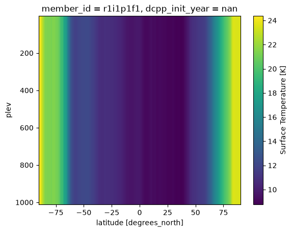
dLW_dts_3d = (regr_kernels.lw_t * tropo_mask(dts_3d) * dp/100).sum(dim='plev', skipna=True)The sum of the two components divided by the change in GMST is the Planck feedback:
planck_feedback = (dLW_ts + dLW_dts_3d)/dgmstplanck_feedback.mean(dim='month').plot(cbar_kwargs={'label': 'W m$^{-2}$ K$^{-1}$'})Could not determine bucket type for bucket name cmip6: Your default credentials were not found. To set up Application Default Credentials, see https://cloud.google.com/docs/authentication/external/set-up-adc for more information., falling back to GCSFileSystem
Could not determine bucket type for bucket name cmip6: Your default credentials were not found. To set up Application Default Credentials, see https://cloud.google.com/docs/authentication/external/set-up-adc for more information., falling back to GCSFileSystem
Could not determine bucket type for bucket name cmip6: Your default credentials were not found. To set up Application Default Credentials, see https://cloud.google.com/docs/authentication/external/set-up-adc for more information., falling back to GCSFileSystem
Could not determine bucket type for bucket name cmip6: Your default credentials were not found. To set up Application Default Credentials, see https://cloud.google.com/docs/authentication/external/set-up-adc for more information., falling back to GCSFileSystem
Could not determine bucket type for bucket name cmip6: Your default credentials were not found. To set up Application Default Credentials, see https://cloud.google.com/docs/authentication/external/set-up-adc for more information., falling back to GCSFileSystem
Could not determine bucket type for bucket name cmip6: Your default credentials were not found. To set up Application Default Credentials, see https://cloud.google.com/docs/authentication/external/set-up-adc for more information., falling back to GCSFileSystem
Could not determine bucket type for bucket name cmip6: Your default credentials were not found. To set up Application Default Credentials, see https://cloud.google.com/docs/authentication/external/set-up-adc for more information., falling back to GCSFileSystem
Could not determine bucket type for bucket name cmip6: Your default credentials were not found. To set up Application Default Credentials, see https://cloud.google.com/docs/authentication/external/set-up-adc for more information., falling back to GCSFileSystem
Could not determine bucket type for bucket name cmip6: Your default credentials were not found. To set up Application Default Credentials, see https://cloud.google.com/docs/authentication/external/set-up-adc for more information., falling back to GCSFileSystem
Could not determine bucket type for bucket name cmip6: Your default credentials were not found. To set up Application Default Credentials, see https://cloud.google.com/docs/authentication/external/set-up-adc for more information., falling back to GCSFileSystem
Could not determine bucket type for bucket name cmip6: Your default credentials were not found. To set up Application Default Credentials, see https://cloud.google.com/docs/authentication/external/set-up-adc for more information., falling back to GCSFileSystem
Could not determine bucket type for bucket name cmip6: Your default credentials were not found. To set up Application Default Credentials, see https://cloud.google.com/docs/authentication/external/set-up-adc for more information., falling back to GCSFileSystem
Could not determine bucket type for bucket name cmip6: Your default credentials were not found. To set up Application Default Credentials, see https://cloud.google.com/docs/authentication/external/set-up-adc for more information., falling back to GCSFileSystem
Could not determine bucket type for bucket name cmip6: Your default credentials were not found. To set up Application Default Credentials, see https://cloud.google.com/docs/authentication/external/set-up-adc for more information., falling back to GCSFileSystem
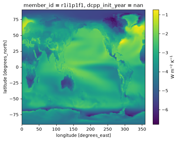
Annual and global average:
gm_planck_feedback = global_average(planck_feedback.mean(dim='month')).load()
gm_planck_feedbackCould not determine bucket type for bucket name cmip6: Your default credentials were not found. To set up Application Default Credentials, see https://cloud.google.com/docs/authentication/external/set-up-adc for more information., falling back to GCSFileSystem
Could not determine bucket type for bucket name cmip6: Your default credentials were not found. To set up Application Default Credentials, see https://cloud.google.com/docs/authentication/external/set-up-adc for more information., falling back to GCSFileSystem
Could not determine bucket type for bucket name cmip6: Your default credentials were not found. To set up Application Default Credentials, see https://cloud.google.com/docs/authentication/external/set-up-adc for more information., falling back to GCSFileSystem
Could not determine bucket type for bucket name cmip6: Your default credentials were not found. To set up Application Default Credentials, see https://cloud.google.com/docs/authentication/external/set-up-adc for more information., falling back to GCSFileSystem
Could not determine bucket type for bucket name cmip6: Your default credentials were not found. To set up Application Default Credentials, see https://cloud.google.com/docs/authentication/external/set-up-adc for more information., falling back to GCSFileSystem
Could not determine bucket type for bucket name cmip6: Your default credentials were not found. To set up Application Default Credentials, see https://cloud.google.com/docs/authentication/external/set-up-adc for more information., falling back to GCSFileSystem
Could not determine bucket type for bucket name cmip6: Your default credentials were not found. To set up Application Default Credentials, see https://cloud.google.com/docs/authentication/external/set-up-adc for more information., falling back to GCSFileSystem
Could not determine bucket type for bucket name cmip6: Your default credentials were not found. To set up Application Default Credentials, see https://cloud.google.com/docs/authentication/external/set-up-adc for more information., falling back to GCSFileSystem
Could not determine bucket type for bucket name cmip6: Your default credentials were not found. To set up Application Default Credentials, see https://cloud.google.com/docs/authentication/external/set-up-adc for more information., falling back to GCSFileSystem
Could not determine bucket type for bucket name cmip6: Your default credentials were not found. To set up Application Default Credentials, see https://cloud.google.com/docs/authentication/external/set-up-adc for more information., falling back to GCSFileSystem
Could not determine bucket type for bucket name cmip6: Your default credentials were not found. To set up Application Default Credentials, see https://cloud.google.com/docs/authentication/external/set-up-adc for more information., falling back to GCSFileSystem
Could not determine bucket type for bucket name cmip6: Your default credentials were not found. To set up Application Default Credentials, see https://cloud.google.com/docs/authentication/external/set-up-adc for more information., falling back to GCSFileSystem
Could not determine bucket type for bucket name cmip6: Your default credentials were not found. To set up Application Default Credentials, see https://cloud.google.com/docs/authentication/external/set-up-adc for more information., falling back to GCSFileSystem
Could not determine bucket type for bucket name cmip6: Your default credentials were not found. To set up Application Default Credentials, see https://cloud.google.com/docs/authentication/external/set-up-adc for more information., falling back to GCSFileSystem
Lapse rate
The lapse rate feedback is calculated using the vertically-nonuniform warming. To do this, we subtract the surface temperature change that we projected into the vertical from the air temperature change, also masking out the stratosphere:
dt_lapserate = tropo_mask(dta - dts_3d)dt_lapserateMultiply by the LW temperature kernel and integrate over pressure:
dLW_lapserate = (regr_kernels.lw_t * tropo_mask(dt_lapserate) * dp/100).sum(dim='plev', skipna=True)Divide by change in GMST to get the feedback:
lapserate_feedback = dLW_lapserate/dgmstlapserate_feedback.mean(dim='month').plot(cbar_kwargs={'label': 'W m$^{-2}$ K$^{-1}$'})Could not determine bucket type for bucket name cmip6: Your default credentials were not found. To set up Application Default Credentials, see https://cloud.google.com/docs/authentication/external/set-up-adc for more information., falling back to GCSFileSystem
Could not determine bucket type for bucket name cmip6: Your default credentials were not found. To set up Application Default Credentials, see https://cloud.google.com/docs/authentication/external/set-up-adc for more information., falling back to GCSFileSystem
Could not determine bucket type for bucket name cmip6: Your default credentials were not found. To set up Application Default Credentials, see https://cloud.google.com/docs/authentication/external/set-up-adc for more information., falling back to GCSFileSystem
Could not determine bucket type for bucket name cmip6: Your default credentials were not found. To set up Application Default Credentials, see https://cloud.google.com/docs/authentication/external/set-up-adc for more information., falling back to GCSFileSystem
Could not determine bucket type for bucket name cmip6: Your default credentials were not found. To set up Application Default Credentials, see https://cloud.google.com/docs/authentication/external/set-up-adc for more information., falling back to GCSFileSystem
Could not determine bucket type for bucket name cmip6: Your default credentials were not found. To set up Application Default Credentials, see https://cloud.google.com/docs/authentication/external/set-up-adc for more information., falling back to GCSFileSystem
Could not determine bucket type for bucket name cmip6: Your default credentials were not found. To set up Application Default Credentials, see https://cloud.google.com/docs/authentication/external/set-up-adc for more information., falling back to GCSFileSystem
Could not determine bucket type for bucket name cmip6: Your default credentials were not found. To set up Application Default Credentials, see https://cloud.google.com/docs/authentication/external/set-up-adc for more information., falling back to GCSFileSystem
Could not determine bucket type for bucket name cmip6: Your default credentials were not found. To set up Application Default Credentials, see https://cloud.google.com/docs/authentication/external/set-up-adc for more information., falling back to GCSFileSystem
Could not determine bucket type for bucket name cmip6: Your default credentials were not found. To set up Application Default Credentials, see https://cloud.google.com/docs/authentication/external/set-up-adc for more information., falling back to GCSFileSystem
Could not determine bucket type for bucket name cmip6: Your default credentials were not found. To set up Application Default Credentials, see https://cloud.google.com/docs/authentication/external/set-up-adc for more information., falling back to GCSFileSystem
Could not determine bucket type for bucket name cmip6: Your default credentials were not found. To set up Application Default Credentials, see https://cloud.google.com/docs/authentication/external/set-up-adc for more information., falling back to GCSFileSystem
Could not determine bucket type for bucket name cmip6: Your default credentials were not found. To set up Application Default Credentials, see https://cloud.google.com/docs/authentication/external/set-up-adc for more information., falling back to GCSFileSystem
Could not determine bucket type for bucket name cmip6: Your default credentials were not found. To set up Application Default Credentials, see https://cloud.google.com/docs/authentication/external/set-up-adc for more information., falling back to GCSFileSystem
Could not determine bucket type for bucket name cmip6: Your default credentials were not found. To set up Application Default Credentials, see https://cloud.google.com/docs/authentication/external/set-up-adc for more information., falling back to GCSFileSystem
Could not determine bucket type for bucket name cmip6: Your default credentials were not found. To set up Application Default Credentials, see https://cloud.google.com/docs/authentication/external/set-up-adc for more information., falling back to GCSFileSystem
Could not determine bucket type for bucket name cmip6: Your default credentials were not found. To set up Application Default Credentials, see https://cloud.google.com/docs/authentication/external/set-up-adc for more information., falling back to GCSFileSystem
Could not determine bucket type for bucket name cmip6: Your default credentials were not found. To set up Application Default Credentials, see https://cloud.google.com/docs/authentication/external/set-up-adc for more information., falling back to GCSFileSystem
Could not determine bucket type for bucket name cmip6: Your default credentials were not found. To set up Application Default Credentials, see https://cloud.google.com/docs/authentication/external/set-up-adc for more information., falling back to GCSFileSystem
Could not determine bucket type for bucket name cmip6: Your default credentials were not found. To set up Application Default Credentials, see https://cloud.google.com/docs/authentication/external/set-up-adc for more information., falling back to GCSFileSystem
Could not determine bucket type for bucket name cmip6: Your default credentials were not found. To set up Application Default Credentials, see https://cloud.google.com/docs/authentication/external/set-up-adc for more information., falling back to GCSFileSystem
Could not determine bucket type for bucket name cmip6: Your default credentials were not found. To set up Application Default Credentials, see https://cloud.google.com/docs/authentication/external/set-up-adc for more information., falling back to GCSFileSystem
Could not determine bucket type for bucket name cmip6: Your default credentials were not found. To set up Application Default Credentials, see https://cloud.google.com/docs/authentication/external/set-up-adc for more information., falling back to GCSFileSystem
Could not determine bucket type for bucket name cmip6: Your default credentials were not found. To set up Application Default Credentials, see https://cloud.google.com/docs/authentication/external/set-up-adc for more information., falling back to GCSFileSystem
Could not determine bucket type for bucket name cmip6: Your default credentials were not found. To set up Application Default Credentials, see https://cloud.google.com/docs/authentication/external/set-up-adc for more information., falling back to GCSFileSystem
Could not determine bucket type for bucket name cmip6: Your default credentials were not found. To set up Application Default Credentials, see https://cloud.google.com/docs/authentication/external/set-up-adc for more information., falling back to GCSFileSystem
Could not determine bucket type for bucket name cmip6: Your default credentials were not found. To set up Application Default Credentials, see https://cloud.google.com/docs/authentication/external/set-up-adc for more information., falling back to GCSFileSystem
Could not determine bucket type for bucket name cmip6: Your default credentials were not found. To set up Application Default Credentials, see https://cloud.google.com/docs/authentication/external/set-up-adc for more information., falling back to GCSFileSystem
Could not determine bucket type for bucket name cmip6: Your default credentials were not found. To set up Application Default Credentials, see https://cloud.google.com/docs/authentication/external/set-up-adc for more information., falling back to GCSFileSystem
Could not determine bucket type for bucket name cmip6: Your default credentials were not found. To set up Application Default Credentials, see https://cloud.google.com/docs/authentication/external/set-up-adc for more information., falling back to GCSFileSystem
Could not determine bucket type for bucket name cmip6: Your default credentials were not found. To set up Application Default Credentials, see https://cloud.google.com/docs/authentication/external/set-up-adc for more information., falling back to GCSFileSystem
Could not determine bucket type for bucket name cmip6: Your default credentials were not found. To set up Application Default Credentials, see https://cloud.google.com/docs/authentication/external/set-up-adc for more information., falling back to GCSFileSystem
Could not determine bucket type for bucket name cmip6: Your default credentials were not found. To set up Application Default Credentials, see https://cloud.google.com/docs/authentication/external/set-up-adc for more information., falling back to GCSFileSystem
Could not determine bucket type for bucket name cmip6: Your default credentials were not found. To set up Application Default Credentials, see https://cloud.google.com/docs/authentication/external/set-up-adc for more information., falling back to GCSFileSystem
Could not determine bucket type for bucket name cmip6: Your default credentials were not found. To set up Application Default Credentials, see https://cloud.google.com/docs/authentication/external/set-up-adc for more information., falling back to GCSFileSystem
Could not determine bucket type for bucket name cmip6: Your default credentials were not found. To set up Application Default Credentials, see https://cloud.google.com/docs/authentication/external/set-up-adc for more information., falling back to GCSFileSystem
Could not determine bucket type for bucket name cmip6: Your default credentials were not found. To set up Application Default Credentials, see https://cloud.google.com/docs/authentication/external/set-up-adc for more information., falling back to GCSFileSystem
Could not determine bucket type for bucket name cmip6: Your default credentials were not found. To set up Application Default Credentials, see https://cloud.google.com/docs/authentication/external/set-up-adc for more information., falling back to GCSFileSystem
Could not determine bucket type for bucket name cmip6: Your default credentials were not found. To set up Application Default Credentials, see https://cloud.google.com/docs/authentication/external/set-up-adc for more information., falling back to GCSFileSystem
Could not determine bucket type for bucket name cmip6: Your default credentials were not found. To set up Application Default Credentials, see https://cloud.google.com/docs/authentication/external/set-up-adc for more information., falling back to GCSFileSystem
Could not determine bucket type for bucket name cmip6: Your default credentials were not found. To set up Application Default Credentials, see https://cloud.google.com/docs/authentication/external/set-up-adc for more information., falling back to GCSFileSystem
Could not determine bucket type for bucket name cmip6: Your default credentials were not found. To set up Application Default Credentials, see https://cloud.google.com/docs/authentication/external/set-up-adc for more information., falling back to GCSFileSystem
Could not determine bucket type for bucket name cmip6: Your default credentials were not found. To set up Application Default Credentials, see https://cloud.google.com/docs/authentication/external/set-up-adc for more information., falling back to GCSFileSystem
Could not determine bucket type for bucket name cmip6: Your default credentials were not found. To set up Application Default Credentials, see https://cloud.google.com/docs/authentication/external/set-up-adc for more information., falling back to GCSFileSystem
Could not determine bucket type for bucket name cmip6: Your default credentials were not found. To set up Application Default Credentials, see https://cloud.google.com/docs/authentication/external/set-up-adc for more information., falling back to GCSFileSystem
Could not determine bucket type for bucket name cmip6: Your default credentials were not found. To set up Application Default Credentials, see https://cloud.google.com/docs/authentication/external/set-up-adc for more information., falling back to GCSFileSystem
Could not determine bucket type for bucket name cmip6: Your default credentials were not found. To set up Application Default Credentials, see https://cloud.google.com/docs/authentication/external/set-up-adc for more information., falling back to GCSFileSystem
Could not determine bucket type for bucket name cmip6: Your default credentials were not found. To set up Application Default Credentials, see https://cloud.google.com/docs/authentication/external/set-up-adc for more information., falling back to GCSFileSystem
Could not determine bucket type for bucket name cmip6: Your default credentials were not found. To set up Application Default Credentials, see https://cloud.google.com/docs/authentication/external/set-up-adc for more information., falling back to GCSFileSystem
Could not determine bucket type for bucket name cmip6: Your default credentials were not found. To set up Application Default Credentials, see https://cloud.google.com/docs/authentication/external/set-up-adc for more information., falling back to GCSFileSystem
Could not determine bucket type for bucket name cmip6: Your default credentials were not found. To set up Application Default Credentials, see https://cloud.google.com/docs/authentication/external/set-up-adc for more information., falling back to GCSFileSystem
Could not determine bucket type for bucket name cmip6: Your default credentials were not found. To set up Application Default Credentials, see https://cloud.google.com/docs/authentication/external/set-up-adc for more information., falling back to GCSFileSystem
Could not determine bucket type for bucket name cmip6: Your default credentials were not found. To set up Application Default Credentials, see https://cloud.google.com/docs/authentication/external/set-up-adc for more information., falling back to GCSFileSystem
Could not determine bucket type for bucket name cmip6: Your default credentials were not found. To set up Application Default Credentials, see https://cloud.google.com/docs/authentication/external/set-up-adc for more information., falling back to GCSFileSystem
Could not determine bucket type for bucket name cmip6: Your default credentials were not found. To set up Application Default Credentials, see https://cloud.google.com/docs/authentication/external/set-up-adc for more information., falling back to GCSFileSystem
Could not determine bucket type for bucket name cmip6: Your default credentials were not found. To set up Application Default Credentials, see https://cloud.google.com/docs/authentication/external/set-up-adc for more information., falling back to GCSFileSystem
Could not determine bucket type for bucket name cmip6: Your default credentials were not found. To set up Application Default Credentials, see https://cloud.google.com/docs/authentication/external/set-up-adc for more information., falling back to GCSFileSystem
Could not determine bucket type for bucket name cmip6: Your default credentials were not found. To set up Application Default Credentials, see https://cloud.google.com/docs/authentication/external/set-up-adc for more information., falling back to GCSFileSystem
Could not determine bucket type for bucket name cmip6: Your default credentials were not found. To set up Application Default Credentials, see https://cloud.google.com/docs/authentication/external/set-up-adc for more information., falling back to GCSFileSystem
Could not determine bucket type for bucket name cmip6: Your default credentials were not found. To set up Application Default Credentials, see https://cloud.google.com/docs/authentication/external/set-up-adc for more information., falling back to GCSFileSystem
Could not determine bucket type for bucket name cmip6: Your default credentials were not found. To set up Application Default Credentials, see https://cloud.google.com/docs/authentication/external/set-up-adc for more information., falling back to GCSFileSystem
Could not determine bucket type for bucket name cmip6: Your default credentials were not found. To set up Application Default Credentials, see https://cloud.google.com/docs/authentication/external/set-up-adc for more information., falling back to GCSFileSystem
Could not determine bucket type for bucket name cmip6: Your default credentials were not found. To set up Application Default Credentials, see https://cloud.google.com/docs/authentication/external/set-up-adc for more information., falling back to GCSFileSystem
Could not determine bucket type for bucket name cmip6: Your default credentials were not found. To set up Application Default Credentials, see https://cloud.google.com/docs/authentication/external/set-up-adc for more information., falling back to GCSFileSystem
Could not determine bucket type for bucket name cmip6: Your default credentials were not found. To set up Application Default Credentials, see https://cloud.google.com/docs/authentication/external/set-up-adc for more information., falling back to GCSFileSystem
Could not determine bucket type for bucket name cmip6: Your default credentials were not found. To set up Application Default Credentials, see https://cloud.google.com/docs/authentication/external/set-up-adc for more information., falling back to GCSFileSystem
Could not determine bucket type for bucket name cmip6: Your default credentials were not found. To set up Application Default Credentials, see https://cloud.google.com/docs/authentication/external/set-up-adc for more information., falling back to GCSFileSystem
Could not determine bucket type for bucket name cmip6: Your default credentials were not found. To set up Application Default Credentials, see https://cloud.google.com/docs/authentication/external/set-up-adc for more information., falling back to GCSFileSystem
Could not determine bucket type for bucket name cmip6: Your default credentials were not found. To set up Application Default Credentials, see https://cloud.google.com/docs/authentication/external/set-up-adc for more information., falling back to GCSFileSystem
Could not determine bucket type for bucket name cmip6: Your default credentials were not found. To set up Application Default Credentials, see https://cloud.google.com/docs/authentication/external/set-up-adc for more information., falling back to GCSFileSystem
Could not determine bucket type for bucket name cmip6: Your default credentials were not found. To set up Application Default Credentials, see https://cloud.google.com/docs/authentication/external/set-up-adc for more information., falling back to GCSFileSystem
Could not determine bucket type for bucket name cmip6: Your default credentials were not found. To set up Application Default Credentials, see https://cloud.google.com/docs/authentication/external/set-up-adc for more information., falling back to GCSFileSystem
Could not determine bucket type for bucket name cmip6: Your default credentials were not found. To set up Application Default Credentials, see https://cloud.google.com/docs/authentication/external/set-up-adc for more information., falling back to GCSFileSystem
Could not determine bucket type for bucket name cmip6: Your default credentials were not found. To set up Application Default Credentials, see https://cloud.google.com/docs/authentication/external/set-up-adc for more information., falling back to GCSFileSystem
Could not determine bucket type for bucket name cmip6: Your default credentials were not found. To set up Application Default Credentials, see https://cloud.google.com/docs/authentication/external/set-up-adc for more information., falling back to GCSFileSystem
Could not determine bucket type for bucket name cmip6: Your default credentials were not found. To set up Application Default Credentials, see https://cloud.google.com/docs/authentication/external/set-up-adc for more information., falling back to GCSFileSystem
Could not determine bucket type for bucket name cmip6: Your default credentials were not found. To set up Application Default Credentials, see https://cloud.google.com/docs/authentication/external/set-up-adc for more information., falling back to GCSFileSystem
Could not determine bucket type for bucket name cmip6: Your default credentials were not found. To set up Application Default Credentials, see https://cloud.google.com/docs/authentication/external/set-up-adc for more information., falling back to GCSFileSystem
Could not determine bucket type for bucket name cmip6: Your default credentials were not found. To set up Application Default Credentials, see https://cloud.google.com/docs/authentication/external/set-up-adc for more information., falling back to GCSFileSystem
Could not determine bucket type for bucket name cmip6: Your default credentials were not found. To set up Application Default Credentials, see https://cloud.google.com/docs/authentication/external/set-up-adc for more information., falling back to GCSFileSystem
Could not determine bucket type for bucket name cmip6: Your default credentials were not found. To set up Application Default Credentials, see https://cloud.google.com/docs/authentication/external/set-up-adc for more information., falling back to GCSFileSystem
Could not determine bucket type for bucket name cmip6: Your default credentials were not found. To set up Application Default Credentials, see https://cloud.google.com/docs/authentication/external/set-up-adc for more information., falling back to GCSFileSystem
Could not determine bucket type for bucket name cmip6: Your default credentials were not found. To set up Application Default Credentials, see https://cloud.google.com/docs/authentication/external/set-up-adc for more information., falling back to GCSFileSystem
Could not determine bucket type for bucket name cmip6: Your default credentials were not found. To set up Application Default Credentials, see https://cloud.google.com/docs/authentication/external/set-up-adc for more information., falling back to GCSFileSystem
Could not determine bucket type for bucket name cmip6: Your default credentials were not found. To set up Application Default Credentials, see https://cloud.google.com/docs/authentication/external/set-up-adc for more information., falling back to GCSFileSystem
Could not determine bucket type for bucket name cmip6: Your default credentials were not found. To set up Application Default Credentials, see https://cloud.google.com/docs/authentication/external/set-up-adc for more information., falling back to GCSFileSystem
Could not determine bucket type for bucket name cmip6: Your default credentials were not found. To set up Application Default Credentials, see https://cloud.google.com/docs/authentication/external/set-up-adc for more information., falling back to GCSFileSystem
Could not determine bucket type for bucket name cmip6: Your default credentials were not found. To set up Application Default Credentials, see https://cloud.google.com/docs/authentication/external/set-up-adc for more information., falling back to GCSFileSystem
Could not determine bucket type for bucket name cmip6: Your default credentials were not found. To set up Application Default Credentials, see https://cloud.google.com/docs/authentication/external/set-up-adc for more information., falling back to GCSFileSystem
Could not determine bucket type for bucket name cmip6: Your default credentials were not found. To set up Application Default Credentials, see https://cloud.google.com/docs/authentication/external/set-up-adc for more information., falling back to GCSFileSystem
Could not determine bucket type for bucket name cmip6: Your default credentials were not found. To set up Application Default Credentials, see https://cloud.google.com/docs/authentication/external/set-up-adc for more information., falling back to GCSFileSystem
Could not determine bucket type for bucket name cmip6: Your default credentials were not found. To set up Application Default Credentials, see https://cloud.google.com/docs/authentication/external/set-up-adc for more information., falling back to GCSFileSystem
Could not determine bucket type for bucket name cmip6: Your default credentials were not found. To set up Application Default Credentials, see https://cloud.google.com/docs/authentication/external/set-up-adc for more information., falling back to GCSFileSystem
Could not determine bucket type for bucket name cmip6: Your default credentials were not found. To set up Application Default Credentials, see https://cloud.google.com/docs/authentication/external/set-up-adc for more information., falling back to GCSFileSystem
Could not determine bucket type for bucket name cmip6: Your default credentials were not found. To set up Application Default Credentials, see https://cloud.google.com/docs/authentication/external/set-up-adc for more information., falling back to GCSFileSystem
Could not determine bucket type for bucket name cmip6: Your default credentials were not found. To set up Application Default Credentials, see https://cloud.google.com/docs/authentication/external/set-up-adc for more information., falling back to GCSFileSystem
Could not determine bucket type for bucket name cmip6: Your default credentials were not found. To set up Application Default Credentials, see https://cloud.google.com/docs/authentication/external/set-up-adc for more information., falling back to GCSFileSystem
Could not determine bucket type for bucket name cmip6: Your default credentials were not found. To set up Application Default Credentials, see https://cloud.google.com/docs/authentication/external/set-up-adc for more information., falling back to GCSFileSystem
Could not determine bucket type for bucket name cmip6: Your default credentials were not found. To set up Application Default Credentials, see https://cloud.google.com/docs/authentication/external/set-up-adc for more information., falling back to GCSFileSystem
Could not determine bucket type for bucket name cmip6: Your default credentials were not found. To set up Application Default Credentials, see https://cloud.google.com/docs/authentication/external/set-up-adc for more information., falling back to GCSFileSystem
Could not determine bucket type for bucket name cmip6: Your default credentials were not found. To set up Application Default Credentials, see https://cloud.google.com/docs/authentication/external/set-up-adc for more information., falling back to GCSFileSystem
Could not determine bucket type for bucket name cmip6: Your default credentials were not found. To set up Application Default Credentials, see https://cloud.google.com/docs/authentication/external/set-up-adc for more information., falling back to GCSFileSystem
Could not determine bucket type for bucket name cmip6: Your default credentials were not found. To set up Application Default Credentials, see https://cloud.google.com/docs/authentication/external/set-up-adc for more information., falling back to GCSFileSystem
Could not determine bucket type for bucket name cmip6: Your default credentials were not found. To set up Application Default Credentials, see https://cloud.google.com/docs/authentication/external/set-up-adc for more information., falling back to GCSFileSystem
Could not determine bucket type for bucket name cmip6: Your default credentials were not found. To set up Application Default Credentials, see https://cloud.google.com/docs/authentication/external/set-up-adc for more information., falling back to GCSFileSystem
Could not determine bucket type for bucket name cmip6: Your default credentials were not found. To set up Application Default Credentials, see https://cloud.google.com/docs/authentication/external/set-up-adc for more information., falling back to GCSFileSystem
Could not determine bucket type for bucket name cmip6: Your default credentials were not found. To set up Application Default Credentials, see https://cloud.google.com/docs/authentication/external/set-up-adc for more information., falling back to GCSFileSystem
Could not determine bucket type for bucket name cmip6: Your default credentials were not found. To set up Application Default Credentials, see https://cloud.google.com/docs/authentication/external/set-up-adc for more information., falling back to GCSFileSystem
Could not determine bucket type for bucket name cmip6: Your default credentials were not found. To set up Application Default Credentials, see https://cloud.google.com/docs/authentication/external/set-up-adc for more information., falling back to GCSFileSystem
Could not determine bucket type for bucket name cmip6: Your default credentials were not found. To set up Application Default Credentials, see https://cloud.google.com/docs/authentication/external/set-up-adc for more information., falling back to GCSFileSystem
Could not determine bucket type for bucket name cmip6: Your default credentials were not found. To set up Application Default Credentials, see https://cloud.google.com/docs/authentication/external/set-up-adc for more information., falling back to GCSFileSystem
Could not determine bucket type for bucket name cmip6: Your default credentials were not found. To set up Application Default Credentials, see https://cloud.google.com/docs/authentication/external/set-up-adc for more information., falling back to GCSFileSystem
Could not determine bucket type for bucket name cmip6: Your default credentials were not found. To set up Application Default Credentials, see https://cloud.google.com/docs/authentication/external/set-up-adc for more information., falling back to GCSFileSystem
Could not determine bucket type for bucket name cmip6: Your default credentials were not found. To set up Application Default Credentials, see https://cloud.google.com/docs/authentication/external/set-up-adc for more information., falling back to GCSFileSystem
Could not determine bucket type for bucket name cmip6: Your default credentials were not found. To set up Application Default Credentials, see https://cloud.google.com/docs/authentication/external/set-up-adc for more information., falling back to GCSFileSystem
Could not determine bucket type for bucket name cmip6: Your default credentials were not found. To set up Application Default Credentials, see https://cloud.google.com/docs/authentication/external/set-up-adc for more information., falling back to GCSFileSystem
Could not determine bucket type for bucket name cmip6: Your default credentials were not found. To set up Application Default Credentials, see https://cloud.google.com/docs/authentication/external/set-up-adc for more information., falling back to GCSFileSystem
Could not determine bucket type for bucket name cmip6: Your default credentials were not found. To set up Application Default Credentials, see https://cloud.google.com/docs/authentication/external/set-up-adc for more information., falling back to GCSFileSystem
Could not determine bucket type for bucket name cmip6: Your default credentials were not found. To set up Application Default Credentials, see https://cloud.google.com/docs/authentication/external/set-up-adc for more information., falling back to GCSFileSystem
Could not determine bucket type for bucket name cmip6: Your default credentials were not found. To set up Application Default Credentials, see https://cloud.google.com/docs/authentication/external/set-up-adc for more information., falling back to GCSFileSystem
Could not determine bucket type for bucket name cmip6: Your default credentials were not found. To set up Application Default Credentials, see https://cloud.google.com/docs/authentication/external/set-up-adc for more information., falling back to GCSFileSystem
Could not determine bucket type for bucket name cmip6: Your default credentials were not found. To set up Application Default Credentials, see https://cloud.google.com/docs/authentication/external/set-up-adc for more information., falling back to GCSFileSystem
Could not determine bucket type for bucket name cmip6: Your default credentials were not found. To set up Application Default Credentials, see https://cloud.google.com/docs/authentication/external/set-up-adc for more information., falling back to GCSFileSystem
Could not determine bucket type for bucket name cmip6: Your default credentials were not found. To set up Application Default Credentials, see https://cloud.google.com/docs/authentication/external/set-up-adc for more information., falling back to GCSFileSystem
Could not determine bucket type for bucket name cmip6: Your default credentials were not found. To set up Application Default Credentials, see https://cloud.google.com/docs/authentication/external/set-up-adc for more information., falling back to GCSFileSystem
Could not determine bucket type for bucket name cmip6: Your default credentials were not found. To set up Application Default Credentials, see https://cloud.google.com/docs/authentication/external/set-up-adc for more information., falling back to GCSFileSystem
Could not determine bucket type for bucket name cmip6: Your default credentials were not found. To set up Application Default Credentials, see https://cloud.google.com/docs/authentication/external/set-up-adc for more information., falling back to GCSFileSystem
Could not determine bucket type for bucket name cmip6: Your default credentials were not found. To set up Application Default Credentials, see https://cloud.google.com/docs/authentication/external/set-up-adc for more information., falling back to GCSFileSystem
Could not determine bucket type for bucket name cmip6: Your default credentials were not found. To set up Application Default Credentials, see https://cloud.google.com/docs/authentication/external/set-up-adc for more information., falling back to GCSFileSystem
Could not determine bucket type for bucket name cmip6: Your default credentials were not found. To set up Application Default Credentials, see https://cloud.google.com/docs/authentication/external/set-up-adc for more information., falling back to GCSFileSystem
Could not determine bucket type for bucket name cmip6: Your default credentials were not found. To set up Application Default Credentials, see https://cloud.google.com/docs/authentication/external/set-up-adc for more information., falling back to GCSFileSystem
Could not determine bucket type for bucket name cmip6: Your default credentials were not found. To set up Application Default Credentials, see https://cloud.google.com/docs/authentication/external/set-up-adc for more information., falling back to GCSFileSystem
Could not determine bucket type for bucket name cmip6: Your default credentials were not found. To set up Application Default Credentials, see https://cloud.google.com/docs/authentication/external/set-up-adc for more information., falling back to GCSFileSystem
Could not determine bucket type for bucket name cmip6: Your default credentials were not found. To set up Application Default Credentials, see https://cloud.google.com/docs/authentication/external/set-up-adc for more information., falling back to GCSFileSystem
Could not determine bucket type for bucket name cmip6: Your default credentials were not found. To set up Application Default Credentials, see https://cloud.google.com/docs/authentication/external/set-up-adc for more information., falling back to GCSFileSystem
Could not determine bucket type for bucket name cmip6: Your default credentials were not found. To set up Application Default Credentials, see https://cloud.google.com/docs/authentication/external/set-up-adc for more information., falling back to GCSFileSystem
Could not determine bucket type for bucket name cmip6: Your default credentials were not found. To set up Application Default Credentials, see https://cloud.google.com/docs/authentication/external/set-up-adc for more information., falling back to GCSFileSystem
Could not determine bucket type for bucket name cmip6: Your default credentials were not found. To set up Application Default Credentials, see https://cloud.google.com/docs/authentication/external/set-up-adc for more information., falling back to GCSFileSystem
Could not determine bucket type for bucket name cmip6: Your default credentials were not found. To set up Application Default Credentials, see https://cloud.google.com/docs/authentication/external/set-up-adc for more information., falling back to GCSFileSystem
Could not determine bucket type for bucket name cmip6: Your default credentials were not found. To set up Application Default Credentials, see https://cloud.google.com/docs/authentication/external/set-up-adc for more information., falling back to GCSFileSystem
Could not determine bucket type for bucket name cmip6: Your default credentials were not found. To set up Application Default Credentials, see https://cloud.google.com/docs/authentication/external/set-up-adc for more information., falling back to GCSFileSystem
Could not determine bucket type for bucket name cmip6: Your default credentials were not found. To set up Application Default Credentials, see https://cloud.google.com/docs/authentication/external/set-up-adc for more information., falling back to GCSFileSystem
Could not determine bucket type for bucket name cmip6: Your default credentials were not found. To set up Application Default Credentials, see https://cloud.google.com/docs/authentication/external/set-up-adc for more information., falling back to GCSFileSystem
Could not determine bucket type for bucket name cmip6: Your default credentials were not found. To set up Application Default Credentials, see https://cloud.google.com/docs/authentication/external/set-up-adc for more information., falling back to GCSFileSystem
Could not determine bucket type for bucket name cmip6: Your default credentials were not found. To set up Application Default Credentials, see https://cloud.google.com/docs/authentication/external/set-up-adc for more information., falling back to GCSFileSystem
Could not determine bucket type for bucket name cmip6: Your default credentials were not found. To set up Application Default Credentials, see https://cloud.google.com/docs/authentication/external/set-up-adc for more information., falling back to GCSFileSystem
Could not determine bucket type for bucket name cmip6: Your default credentials were not found. To set up Application Default Credentials, see https://cloud.google.com/docs/authentication/external/set-up-adc for more information., falling back to GCSFileSystem
Could not determine bucket type for bucket name cmip6: Your default credentials were not found. To set up Application Default Credentials, see https://cloud.google.com/docs/authentication/external/set-up-adc for more information., falling back to GCSFileSystem
Could not determine bucket type for bucket name cmip6: Your default credentials were not found. To set up Application Default Credentials, see https://cloud.google.com/docs/authentication/external/set-up-adc for more information., falling back to GCSFileSystem
Could not determine bucket type for bucket name cmip6: Your default credentials were not found. To set up Application Default Credentials, see https://cloud.google.com/docs/authentication/external/set-up-adc for more information., falling back to GCSFileSystem
Could not determine bucket type for bucket name cmip6: Your default credentials were not found. To set up Application Default Credentials, see https://cloud.google.com/docs/authentication/external/set-up-adc for more information., falling back to GCSFileSystem
Could not determine bucket type for bucket name cmip6: Your default credentials were not found. To set up Application Default Credentials, see https://cloud.google.com/docs/authentication/external/set-up-adc for more information., falling back to GCSFileSystem
Could not determine bucket type for bucket name cmip6: Your default credentials were not found. To set up Application Default Credentials, see https://cloud.google.com/docs/authentication/external/set-up-adc for more information., falling back to GCSFileSystem
Could not determine bucket type for bucket name cmip6: Your default credentials were not found. To set up Application Default Credentials, see https://cloud.google.com/docs/authentication/external/set-up-adc for more information., falling back to GCSFileSystem
Could not determine bucket type for bucket name cmip6: Your default credentials were not found. To set up Application Default Credentials, see https://cloud.google.com/docs/authentication/external/set-up-adc for more information., falling back to GCSFileSystem
Could not determine bucket type for bucket name cmip6: Your default credentials were not found. To set up Application Default Credentials, see https://cloud.google.com/docs/authentication/external/set-up-adc for more information., falling back to GCSFileSystem
Could not determine bucket type for bucket name cmip6: Your default credentials were not found. To set up Application Default Credentials, see https://cloud.google.com/docs/authentication/external/set-up-adc for more information., falling back to GCSFileSystem
Could not determine bucket type for bucket name cmip6: Your default credentials were not found. To set up Application Default Credentials, see https://cloud.google.com/docs/authentication/external/set-up-adc for more information., falling back to GCSFileSystem
Could not determine bucket type for bucket name cmip6: Your default credentials were not found. To set up Application Default Credentials, see https://cloud.google.com/docs/authentication/external/set-up-adc for more information., falling back to GCSFileSystem
Could not determine bucket type for bucket name cmip6: Your default credentials were not found. To set up Application Default Credentials, see https://cloud.google.com/docs/authentication/external/set-up-adc for more information., falling back to GCSFileSystem
Could not determine bucket type for bucket name cmip6: Your default credentials were not found. To set up Application Default Credentials, see https://cloud.google.com/docs/authentication/external/set-up-adc for more information., falling back to GCSFileSystem
Could not determine bucket type for bucket name cmip6: Your default credentials were not found. To set up Application Default Credentials, see https://cloud.google.com/docs/authentication/external/set-up-adc for more information., falling back to GCSFileSystem
Could not determine bucket type for bucket name cmip6: Your default credentials were not found. To set up Application Default Credentials, see https://cloud.google.com/docs/authentication/external/set-up-adc for more information., falling back to GCSFileSystem
Could not determine bucket type for bucket name cmip6: Your default credentials were not found. To set up Application Default Credentials, see https://cloud.google.com/docs/authentication/external/set-up-adc for more information., falling back to GCSFileSystem
Could not determine bucket type for bucket name cmip6: Your default credentials were not found. To set up Application Default Credentials, see https://cloud.google.com/docs/authentication/external/set-up-adc for more information., falling back to GCSFileSystem
Could not determine bucket type for bucket name cmip6: Your default credentials were not found. To set up Application Default Credentials, see https://cloud.google.com/docs/authentication/external/set-up-adc for more information., falling back to GCSFileSystem
Could not determine bucket type for bucket name cmip6: Your default credentials were not found. To set up Application Default Credentials, see https://cloud.google.com/docs/authentication/external/set-up-adc for more information., falling back to GCSFileSystem
Could not determine bucket type for bucket name cmip6: Your default credentials were not found. To set up Application Default Credentials, see https://cloud.google.com/docs/authentication/external/set-up-adc for more information., falling back to GCSFileSystem
Could not determine bucket type for bucket name cmip6: Your default credentials were not found. To set up Application Default Credentials, see https://cloud.google.com/docs/authentication/external/set-up-adc for more information., falling back to GCSFileSystem
Could not determine bucket type for bucket name cmip6: Your default credentials were not found. To set up Application Default Credentials, see https://cloud.google.com/docs/authentication/external/set-up-adc for more information., falling back to GCSFileSystem
Could not determine bucket type for bucket name cmip6: Your default credentials were not found. To set up Application Default Credentials, see https://cloud.google.com/docs/authentication/external/set-up-adc for more information., falling back to GCSFileSystem
Could not determine bucket type for bucket name cmip6: Your default credentials were not found. To set up Application Default Credentials, see https://cloud.google.com/docs/authentication/external/set-up-adc for more information., falling back to GCSFileSystem
Could not determine bucket type for bucket name cmip6: Your default credentials were not found. To set up Application Default Credentials, see https://cloud.google.com/docs/authentication/external/set-up-adc for more information., falling back to GCSFileSystem
Could not determine bucket type for bucket name cmip6: Your default credentials were not found. To set up Application Default Credentials, see https://cloud.google.com/docs/authentication/external/set-up-adc for more information., falling back to GCSFileSystem
Could not determine bucket type for bucket name cmip6: Your default credentials were not found. To set up Application Default Credentials, see https://cloud.google.com/docs/authentication/external/set-up-adc for more information., falling back to GCSFileSystem
Could not determine bucket type for bucket name cmip6: Your default credentials were not found. To set up Application Default Credentials, see https://cloud.google.com/docs/authentication/external/set-up-adc for more information., falling back to GCSFileSystem
Could not determine bucket type for bucket name cmip6: Your default credentials were not found. To set up Application Default Credentials, see https://cloud.google.com/docs/authentication/external/set-up-adc for more information., falling back to GCSFileSystem
Could not determine bucket type for bucket name cmip6: Your default credentials were not found. To set up Application Default Credentials, see https://cloud.google.com/docs/authentication/external/set-up-adc for more information., falling back to GCSFileSystem
Could not determine bucket type for bucket name cmip6: Your default credentials were not found. To set up Application Default Credentials, see https://cloud.google.com/docs/authentication/external/set-up-adc for more information., falling back to GCSFileSystem
Could not determine bucket type for bucket name cmip6: Your default credentials were not found. To set up Application Default Credentials, see https://cloud.google.com/docs/authentication/external/set-up-adc for more information., falling back to GCSFileSystem
Could not determine bucket type for bucket name cmip6: Your default credentials were not found. To set up Application Default Credentials, see https://cloud.google.com/docs/authentication/external/set-up-adc for more information., falling back to GCSFileSystem
Could not determine bucket type for bucket name cmip6: Your default credentials were not found. To set up Application Default Credentials, see https://cloud.google.com/docs/authentication/external/set-up-adc for more information., falling back to GCSFileSystem
Could not determine bucket type for bucket name cmip6: Your default credentials were not found. To set up Application Default Credentials, see https://cloud.google.com/docs/authentication/external/set-up-adc for more information., falling back to GCSFileSystem
Could not determine bucket type for bucket name cmip6: Your default credentials were not found. To set up Application Default Credentials, see https://cloud.google.com/docs/authentication/external/set-up-adc for more information., falling back to GCSFileSystem
Could not determine bucket type for bucket name cmip6: Your default credentials were not found. To set up Application Default Credentials, see https://cloud.google.com/docs/authentication/external/set-up-adc for more information., falling back to GCSFileSystem
Could not determine bucket type for bucket name cmip6: Your default credentials were not found. To set up Application Default Credentials, see https://cloud.google.com/docs/authentication/external/set-up-adc for more information., falling back to GCSFileSystem
Could not determine bucket type for bucket name cmip6: Your default credentials were not found. To set up Application Default Credentials, see https://cloud.google.com/docs/authentication/external/set-up-adc for more information., falling back to GCSFileSystem
Could not determine bucket type for bucket name cmip6: Your default credentials were not found. To set up Application Default Credentials, see https://cloud.google.com/docs/authentication/external/set-up-adc for more information., falling back to GCSFileSystem
Could not determine bucket type for bucket name cmip6: Your default credentials were not found. To set up Application Default Credentials, see https://cloud.google.com/docs/authentication/external/set-up-adc for more information., falling back to GCSFileSystem
Could not determine bucket type for bucket name cmip6: Your default credentials were not found. To set up Application Default Credentials, see https://cloud.google.com/docs/authentication/external/set-up-adc for more information., falling back to GCSFileSystem
Could not determine bucket type for bucket name cmip6: Your default credentials were not found. To set up Application Default Credentials, see https://cloud.google.com/docs/authentication/external/set-up-adc for more information., falling back to GCSFileSystem
Could not determine bucket type for bucket name cmip6: Your default credentials were not found. To set up Application Default Credentials, see https://cloud.google.com/docs/authentication/external/set-up-adc for more information., falling back to GCSFileSystem
Could not determine bucket type for bucket name cmip6: Your default credentials were not found. To set up Application Default Credentials, see https://cloud.google.com/docs/authentication/external/set-up-adc for more information., falling back to GCSFileSystem
Could not determine bucket type for bucket name cmip6: Your default credentials were not found. To set up Application Default Credentials, see https://cloud.google.com/docs/authentication/external/set-up-adc for more information., falling back to GCSFileSystem
Could not determine bucket type for bucket name cmip6: Your default credentials were not found. To set up Application Default Credentials, see https://cloud.google.com/docs/authentication/external/set-up-adc for more information., falling back to GCSFileSystem
Could not determine bucket type for bucket name cmip6: Your default credentials were not found. To set up Application Default Credentials, see https://cloud.google.com/docs/authentication/external/set-up-adc for more information., falling back to GCSFileSystem
Could not determine bucket type for bucket name cmip6: Your default credentials were not found. To set up Application Default Credentials, see https://cloud.google.com/docs/authentication/external/set-up-adc for more information., falling back to GCSFileSystem
Could not determine bucket type for bucket name cmip6: Your default credentials were not found. To set up Application Default Credentials, see https://cloud.google.com/docs/authentication/external/set-up-adc for more information., falling back to GCSFileSystem
Could not determine bucket type for bucket name cmip6: Your default credentials were not found. To set up Application Default Credentials, see https://cloud.google.com/docs/authentication/external/set-up-adc for more information., falling back to GCSFileSystem
Could not determine bucket type for bucket name cmip6: Your default credentials were not found. To set up Application Default Credentials, see https://cloud.google.com/docs/authentication/external/set-up-adc for more information., falling back to GCSFileSystem
Could not determine bucket type for bucket name cmip6: Your default credentials were not found. To set up Application Default Credentials, see https://cloud.google.com/docs/authentication/external/set-up-adc for more information., falling back to GCSFileSystem
Could not determine bucket type for bucket name cmip6: Your default credentials were not found. To set up Application Default Credentials, see https://cloud.google.com/docs/authentication/external/set-up-adc for more information., falling back to GCSFileSystem
Could not determine bucket type for bucket name cmip6: Your default credentials were not found. To set up Application Default Credentials, see https://cloud.google.com/docs/authentication/external/set-up-adc for more information., falling back to GCSFileSystem
Could not determine bucket type for bucket name cmip6: Your default credentials were not found. To set up Application Default Credentials, see https://cloud.google.com/docs/authentication/external/set-up-adc for more information., falling back to GCSFileSystem
Could not determine bucket type for bucket name cmip6: Your default credentials were not found. To set up Application Default Credentials, see https://cloud.google.com/docs/authentication/external/set-up-adc for more information., falling back to GCSFileSystem
Could not determine bucket type for bucket name cmip6: Your default credentials were not found. To set up Application Default Credentials, see https://cloud.google.com/docs/authentication/external/set-up-adc for more information., falling back to GCSFileSystem
Could not determine bucket type for bucket name cmip6: Your default credentials were not found. To set up Application Default Credentials, see https://cloud.google.com/docs/authentication/external/set-up-adc for more information., falling back to GCSFileSystem
Could not determine bucket type for bucket name cmip6: Your default credentials were not found. To set up Application Default Credentials, see https://cloud.google.com/docs/authentication/external/set-up-adc for more information., falling back to GCSFileSystem
Could not determine bucket type for bucket name cmip6: Your default credentials were not found. To set up Application Default Credentials, see https://cloud.google.com/docs/authentication/external/set-up-adc for more information., falling back to GCSFileSystem
Could not determine bucket type for bucket name cmip6: Your default credentials were not found. To set up Application Default Credentials, see https://cloud.google.com/docs/authentication/external/set-up-adc for more information., falling back to GCSFileSystem
Could not determine bucket type for bucket name cmip6: Your default credentials were not found. To set up Application Default Credentials, see https://cloud.google.com/docs/authentication/external/set-up-adc for more information., falling back to GCSFileSystem
Could not determine bucket type for bucket name cmip6: Your default credentials were not found. To set up Application Default Credentials, see https://cloud.google.com/docs/authentication/external/set-up-adc for more information., falling back to GCSFileSystem
Could not determine bucket type for bucket name cmip6: Your default credentials were not found. To set up Application Default Credentials, see https://cloud.google.com/docs/authentication/external/set-up-adc for more information., falling back to GCSFileSystem
Could not determine bucket type for bucket name cmip6: Your default credentials were not found. To set up Application Default Credentials, see https://cloud.google.com/docs/authentication/external/set-up-adc for more information., falling back to GCSFileSystem
Could not determine bucket type for bucket name cmip6: Your default credentials were not found. To set up Application Default Credentials, see https://cloud.google.com/docs/authentication/external/set-up-adc for more information., falling back to GCSFileSystem
Could not determine bucket type for bucket name cmip6: Your default credentials were not found. To set up Application Default Credentials, see https://cloud.google.com/docs/authentication/external/set-up-adc for more information., falling back to GCSFileSystem
Could not determine bucket type for bucket name cmip6: Your default credentials were not found. To set up Application Default Credentials, see https://cloud.google.com/docs/authentication/external/set-up-adc for more information., falling back to GCSFileSystem
Could not determine bucket type for bucket name cmip6: Your default credentials were not found. To set up Application Default Credentials, see https://cloud.google.com/docs/authentication/external/set-up-adc for more information., falling back to GCSFileSystem
Could not determine bucket type for bucket name cmip6: Your default credentials were not found. To set up Application Default Credentials, see https://cloud.google.com/docs/authentication/external/set-up-adc for more information., falling back to GCSFileSystem
Could not determine bucket type for bucket name cmip6: Your default credentials were not found. To set up Application Default Credentials, see https://cloud.google.com/docs/authentication/external/set-up-adc for more information., falling back to GCSFileSystem
Could not determine bucket type for bucket name cmip6: Your default credentials were not found. To set up Application Default Credentials, see https://cloud.google.com/docs/authentication/external/set-up-adc for more information., falling back to GCSFileSystem
Could not determine bucket type for bucket name cmip6: Your default credentials were not found. To set up Application Default Credentials, see https://cloud.google.com/docs/authentication/external/set-up-adc for more information., falling back to GCSFileSystem
Could not determine bucket type for bucket name cmip6: Your default credentials were not found. To set up Application Default Credentials, see https://cloud.google.com/docs/authentication/external/set-up-adc for more information., falling back to GCSFileSystem
Could not determine bucket type for bucket name cmip6: Your default credentials were not found. To set up Application Default Credentials, see https://cloud.google.com/docs/authentication/external/set-up-adc for more information., falling back to GCSFileSystem
Could not determine bucket type for bucket name cmip6: Your default credentials were not found. To set up Application Default Credentials, see https://cloud.google.com/docs/authentication/external/set-up-adc for more information., falling back to GCSFileSystem
Could not determine bucket type for bucket name cmip6: Your default credentials were not found. To set up Application Default Credentials, see https://cloud.google.com/docs/authentication/external/set-up-adc for more information., falling back to GCSFileSystem
Could not determine bucket type for bucket name cmip6: Your default credentials were not found. To set up Application Default Credentials, see https://cloud.google.com/docs/authentication/external/set-up-adc for more information., falling back to GCSFileSystem
Could not determine bucket type for bucket name cmip6: Your default credentials were not found. To set up Application Default Credentials, see https://cloud.google.com/docs/authentication/external/set-up-adc for more information., falling back to GCSFileSystem
Could not determine bucket type for bucket name cmip6: Your default credentials were not found. To set up Application Default Credentials, see https://cloud.google.com/docs/authentication/external/set-up-adc for more information., falling back to GCSFileSystem
Could not determine bucket type for bucket name cmip6: Your default credentials were not found. To set up Application Default Credentials, see https://cloud.google.com/docs/authentication/external/set-up-adc for more information., falling back to GCSFileSystem
Could not determine bucket type for bucket name cmip6: Your default credentials were not found. To set up Application Default Credentials, see https://cloud.google.com/docs/authentication/external/set-up-adc for more information., falling back to GCSFileSystem
Could not determine bucket type for bucket name cmip6: Your default credentials were not found. To set up Application Default Credentials, see https://cloud.google.com/docs/authentication/external/set-up-adc for more information., falling back to GCSFileSystem
Could not determine bucket type for bucket name cmip6: Your default credentials were not found. To set up Application Default Credentials, see https://cloud.google.com/docs/authentication/external/set-up-adc for more information., falling back to GCSFileSystem
Could not determine bucket type for bucket name cmip6: Your default credentials were not found. To set up Application Default Credentials, see https://cloud.google.com/docs/authentication/external/set-up-adc for more information., falling back to GCSFileSystem
Could not determine bucket type for bucket name cmip6: Your default credentials were not found. To set up Application Default Credentials, see https://cloud.google.com/docs/authentication/external/set-up-adc for more information., falling back to GCSFileSystem
Could not determine bucket type for bucket name cmip6: Your default credentials were not found. To set up Application Default Credentials, see https://cloud.google.com/docs/authentication/external/set-up-adc for more information., falling back to GCSFileSystem
Could not determine bucket type for bucket name cmip6: Your default credentials were not found. To set up Application Default Credentials, see https://cloud.google.com/docs/authentication/external/set-up-adc for more information., falling back to GCSFileSystem
Could not determine bucket type for bucket name cmip6: Your default credentials were not found. To set up Application Default Credentials, see https://cloud.google.com/docs/authentication/external/set-up-adc for more information., falling back to GCSFileSystem
Could not determine bucket type for bucket name cmip6: Your default credentials were not found. To set up Application Default Credentials, see https://cloud.google.com/docs/authentication/external/set-up-adc for more information., falling back to GCSFileSystem
Could not determine bucket type for bucket name cmip6: Your default credentials were not found. To set up Application Default Credentials, see https://cloud.google.com/docs/authentication/external/set-up-adc for more information., falling back to GCSFileSystem
Could not determine bucket type for bucket name cmip6: Your default credentials were not found. To set up Application Default Credentials, see https://cloud.google.com/docs/authentication/external/set-up-adc for more information., falling back to GCSFileSystem
Could not determine bucket type for bucket name cmip6: Your default credentials were not found. To set up Application Default Credentials, see https://cloud.google.com/docs/authentication/external/set-up-adc for more information., falling back to GCSFileSystem
Could not determine bucket type for bucket name cmip6: Your default credentials were not found. To set up Application Default Credentials, see https://cloud.google.com/docs/authentication/external/set-up-adc for more information., falling back to GCSFileSystem
Could not determine bucket type for bucket name cmip6: Your default credentials were not found. To set up Application Default Credentials, see https://cloud.google.com/docs/authentication/external/set-up-adc for more information., falling back to GCSFileSystem
Could not determine bucket type for bucket name cmip6: Your default credentials were not found. To set up Application Default Credentials, see https://cloud.google.com/docs/authentication/external/set-up-adc for more information., falling back to GCSFileSystem
Could not determine bucket type for bucket name cmip6: Your default credentials were not found. To set up Application Default Credentials, see https://cloud.google.com/docs/authentication/external/set-up-adc for more information., falling back to GCSFileSystem
Could not determine bucket type for bucket name cmip6: Your default credentials were not found. To set up Application Default Credentials, see https://cloud.google.com/docs/authentication/external/set-up-adc for more information., falling back to GCSFileSystem
Could not determine bucket type for bucket name cmip6: Your default credentials were not found. To set up Application Default Credentials, see https://cloud.google.com/docs/authentication/external/set-up-adc for more information., falling back to GCSFileSystem
Could not determine bucket type for bucket name cmip6: Your default credentials were not found. To set up Application Default Credentials, see https://cloud.google.com/docs/authentication/external/set-up-adc for more information., falling back to GCSFileSystem
Could not determine bucket type for bucket name cmip6: Your default credentials were not found. To set up Application Default Credentials, see https://cloud.google.com/docs/authentication/external/set-up-adc for more information., falling back to GCSFileSystem
Could not determine bucket type for bucket name cmip6: Your default credentials were not found. To set up Application Default Credentials, see https://cloud.google.com/docs/authentication/external/set-up-adc for more information., falling back to GCSFileSystem
Could not determine bucket type for bucket name cmip6: Your default credentials were not found. To set up Application Default Credentials, see https://cloud.google.com/docs/authentication/external/set-up-adc for more information., falling back to GCSFileSystem
Could not determine bucket type for bucket name cmip6: Your default credentials were not found. To set up Application Default Credentials, see https://cloud.google.com/docs/authentication/external/set-up-adc for more information., falling back to GCSFileSystem
Could not determine bucket type for bucket name cmip6: Your default credentials were not found. To set up Application Default Credentials, see https://cloud.google.com/docs/authentication/external/set-up-adc for more information., falling back to GCSFileSystem
Could not determine bucket type for bucket name cmip6: Your default credentials were not found. To set up Application Default Credentials, see https://cloud.google.com/docs/authentication/external/set-up-adc for more information., falling back to GCSFileSystem
Could not determine bucket type for bucket name cmip6: Your default credentials were not found. To set up Application Default Credentials, see https://cloud.google.com/docs/authentication/external/set-up-adc for more information., falling back to GCSFileSystem
Could not determine bucket type for bucket name cmip6: Your default credentials were not found. To set up Application Default Credentials, see https://cloud.google.com/docs/authentication/external/set-up-adc for more information., falling back to GCSFileSystem
Could not determine bucket type for bucket name cmip6: Your default credentials were not found. To set up Application Default Credentials, see https://cloud.google.com/docs/authentication/external/set-up-adc for more information., falling back to GCSFileSystem
Could not determine bucket type for bucket name cmip6: Your default credentials were not found. To set up Application Default Credentials, see https://cloud.google.com/docs/authentication/external/set-up-adc for more information., falling back to GCSFileSystem
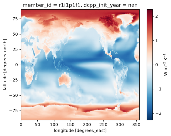
Global average:
gm_lapserate_feedback = global_average(lapserate_feedback.mean(dim='month')).load()
gm_lapserate_feedbackCould not determine bucket type for bucket name cmip6: Your default credentials were not found. To set up Application Default Credentials, see https://cloud.google.com/docs/authentication/external/set-up-adc for more information., falling back to GCSFileSystem
Could not determine bucket type for bucket name cmip6: Your default credentials were not found. To set up Application Default Credentials, see https://cloud.google.com/docs/authentication/external/set-up-adc for more information., falling back to GCSFileSystem
Could not determine bucket type for bucket name cmip6: Your default credentials were not found. To set up Application Default Credentials, see https://cloud.google.com/docs/authentication/external/set-up-adc for more information., falling back to GCSFileSystem
Could not determine bucket type for bucket name cmip6: Your default credentials were not found. To set up Application Default Credentials, see https://cloud.google.com/docs/authentication/external/set-up-adc for more information., falling back to GCSFileSystem
Could not determine bucket type for bucket name cmip6: Your default credentials were not found. To set up Application Default Credentials, see https://cloud.google.com/docs/authentication/external/set-up-adc for more information., falling back to GCSFileSystem
Could not determine bucket type for bucket name cmip6: Your default credentials were not found. To set up Application Default Credentials, see https://cloud.google.com/docs/authentication/external/set-up-adc for more information., falling back to GCSFileSystem
Could not determine bucket type for bucket name cmip6: Your default credentials were not found. To set up Application Default Credentials, see https://cloud.google.com/docs/authentication/external/set-up-adc for more information., falling back to GCSFileSystem
Could not determine bucket type for bucket name cmip6: Your default credentials were not found. To set up Application Default Credentials, see https://cloud.google.com/docs/authentication/external/set-up-adc for more information., falling back to GCSFileSystem
Could not determine bucket type for bucket name cmip6: Your default credentials were not found. To set up Application Default Credentials, see https://cloud.google.com/docs/authentication/external/set-up-adc for more information., falling back to GCSFileSystem
Could not determine bucket type for bucket name cmip6: Your default credentials were not found. To set up Application Default Credentials, see https://cloud.google.com/docs/authentication/external/set-up-adc for more information., falling back to GCSFileSystem
Could not determine bucket type for bucket name cmip6: Your default credentials were not found. To set up Application Default Credentials, see https://cloud.google.com/docs/authentication/external/set-up-adc for more information., falling back to GCSFileSystem
Could not determine bucket type for bucket name cmip6: Your default credentials were not found. To set up Application Default Credentials, see https://cloud.google.com/docs/authentication/external/set-up-adc for more information., falling back to GCSFileSystem
Could not determine bucket type for bucket name cmip6: Your default credentials were not found. To set up Application Default Credentials, see https://cloud.google.com/docs/authentication/external/set-up-adc for more information., falling back to GCSFileSystem
Could not determine bucket type for bucket name cmip6: Your default credentials were not found. To set up Application Default Credentials, see https://cloud.google.com/docs/authentication/external/set-up-adc for more information., falling back to GCSFileSystem
Could not determine bucket type for bucket name cmip6: Your default credentials were not found. To set up Application Default Credentials, see https://cloud.google.com/docs/authentication/external/set-up-adc for more information., falling back to GCSFileSystem
Could not determine bucket type for bucket name cmip6: Your default credentials were not found. To set up Application Default Credentials, see https://cloud.google.com/docs/authentication/external/set-up-adc for more information., falling back to GCSFileSystem
Could not determine bucket type for bucket name cmip6: Your default credentials were not found. To set up Application Default Credentials, see https://cloud.google.com/docs/authentication/external/set-up-adc for more information., falling back to GCSFileSystem
Could not determine bucket type for bucket name cmip6: Your default credentials were not found. To set up Application Default Credentials, see https://cloud.google.com/docs/authentication/external/set-up-adc for more information., falling back to GCSFileSystem
Could not determine bucket type for bucket name cmip6: Your default credentials were not found. To set up Application Default Credentials, see https://cloud.google.com/docs/authentication/external/set-up-adc for more information., falling back to GCSFileSystem
Could not determine bucket type for bucket name cmip6: Your default credentials were not found. To set up Application Default Credentials, see https://cloud.google.com/docs/authentication/external/set-up-adc for more information., falling back to GCSFileSystem
Could not determine bucket type for bucket name cmip6: Your default credentials were not found. To set up Application Default Credentials, see https://cloud.google.com/docs/authentication/external/set-up-adc for more information., falling back to GCSFileSystem
Could not determine bucket type for bucket name cmip6: Your default credentials were not found. To set up Application Default Credentials, see https://cloud.google.com/docs/authentication/external/set-up-adc for more information., falling back to GCSFileSystem
Could not determine bucket type for bucket name cmip6: Your default credentials were not found. To set up Application Default Credentials, see https://cloud.google.com/docs/authentication/external/set-up-adc for more information., falling back to GCSFileSystem
Could not determine bucket type for bucket name cmip6: Your default credentials were not found. To set up Application Default Credentials, see https://cloud.google.com/docs/authentication/external/set-up-adc for more information., falling back to GCSFileSystem
Could not determine bucket type for bucket name cmip6: Your default credentials were not found. To set up Application Default Credentials, see https://cloud.google.com/docs/authentication/external/set-up-adc for more information., falling back to GCSFileSystem
Could not determine bucket type for bucket name cmip6: Your default credentials were not found. To set up Application Default Credentials, see https://cloud.google.com/docs/authentication/external/set-up-adc for more information., falling back to GCSFileSystem
Could not determine bucket type for bucket name cmip6: Your default credentials were not found. To set up Application Default Credentials, see https://cloud.google.com/docs/authentication/external/set-up-adc for more information., falling back to GCSFileSystem
Could not determine bucket type for bucket name cmip6: Your default credentials were not found. To set up Application Default Credentials, see https://cloud.google.com/docs/authentication/external/set-up-adc for more information., falling back to GCSFileSystem
Could not determine bucket type for bucket name cmip6: Your default credentials were not found. To set up Application Default Credentials, see https://cloud.google.com/docs/authentication/external/set-up-adc for more information., falling back to GCSFileSystem
Could not determine bucket type for bucket name cmip6: Your default credentials were not found. To set up Application Default Credentials, see https://cloud.google.com/docs/authentication/external/set-up-adc for more information., falling back to GCSFileSystem
Could not determine bucket type for bucket name cmip6: Your default credentials were not found. To set up Application Default Credentials, see https://cloud.google.com/docs/authentication/external/set-up-adc for more information., falling back to GCSFileSystem
Could not determine bucket type for bucket name cmip6: Your default credentials were not found. To set up Application Default Credentials, see https://cloud.google.com/docs/authentication/external/set-up-adc for more information., falling back to GCSFileSystem
Could not determine bucket type for bucket name cmip6: Your default credentials were not found. To set up Application Default Credentials, see https://cloud.google.com/docs/authentication/external/set-up-adc for more information., falling back to GCSFileSystem
Could not determine bucket type for bucket name cmip6: Your default credentials were not found. To set up Application Default Credentials, see https://cloud.google.com/docs/authentication/external/set-up-adc for more information., falling back to GCSFileSystem
Could not determine bucket type for bucket name cmip6: Your default credentials were not found. To set up Application Default Credentials, see https://cloud.google.com/docs/authentication/external/set-up-adc for more information., falling back to GCSFileSystem
Could not determine bucket type for bucket name cmip6: Your default credentials were not found. To set up Application Default Credentials, see https://cloud.google.com/docs/authentication/external/set-up-adc for more information., falling back to GCSFileSystem
Could not determine bucket type for bucket name cmip6: Your default credentials were not found. To set up Application Default Credentials, see https://cloud.google.com/docs/authentication/external/set-up-adc for more information., falling back to GCSFileSystem
Could not determine bucket type for bucket name cmip6: Your default credentials were not found. To set up Application Default Credentials, see https://cloud.google.com/docs/authentication/external/set-up-adc for more information., falling back to GCSFileSystem
Could not determine bucket type for bucket name cmip6: Your default credentials were not found. To set up Application Default Credentials, see https://cloud.google.com/docs/authentication/external/set-up-adc for more information., falling back to GCSFileSystem
Could not determine bucket type for bucket name cmip6: Your default credentials were not found. To set up Application Default Credentials, see https://cloud.google.com/docs/authentication/external/set-up-adc for more information., falling back to GCSFileSystem
Could not determine bucket type for bucket name cmip6: Your default credentials were not found. To set up Application Default Credentials, see https://cloud.google.com/docs/authentication/external/set-up-adc for more information., falling back to GCSFileSystem
Could not determine bucket type for bucket name cmip6: Your default credentials were not found. To set up Application Default Credentials, see https://cloud.google.com/docs/authentication/external/set-up-adc for more information., falling back to GCSFileSystem
Could not determine bucket type for bucket name cmip6: Your default credentials were not found. To set up Application Default Credentials, see https://cloud.google.com/docs/authentication/external/set-up-adc for more information., falling back to GCSFileSystem
Could not determine bucket type for bucket name cmip6: Your default credentials were not found. To set up Application Default Credentials, see https://cloud.google.com/docs/authentication/external/set-up-adc for more information., falling back to GCSFileSystem
Could not determine bucket type for bucket name cmip6: Your default credentials were not found. To set up Application Default Credentials, see https://cloud.google.com/docs/authentication/external/set-up-adc for more information., falling back to GCSFileSystem
Could not determine bucket type for bucket name cmip6: Your default credentials were not found. To set up Application Default Credentials, see https://cloud.google.com/docs/authentication/external/set-up-adc for more information., falling back to GCSFileSystem
Could not determine bucket type for bucket name cmip6: Your default credentials were not found. To set up Application Default Credentials, see https://cloud.google.com/docs/authentication/external/set-up-adc for more information., falling back to GCSFileSystem
Could not determine bucket type for bucket name cmip6: Your default credentials were not found. To set up Application Default Credentials, see https://cloud.google.com/docs/authentication/external/set-up-adc for more information., falling back to GCSFileSystem
Could not determine bucket type for bucket name cmip6: Your default credentials were not found. To set up Application Default Credentials, see https://cloud.google.com/docs/authentication/external/set-up-adc for more information., falling back to GCSFileSystem
Could not determine bucket type for bucket name cmip6: Your default credentials were not found. To set up Application Default Credentials, see https://cloud.google.com/docs/authentication/external/set-up-adc for more information., falling back to GCSFileSystem
Could not determine bucket type for bucket name cmip6: Your default credentials were not found. To set up Application Default Credentials, see https://cloud.google.com/docs/authentication/external/set-up-adc for more information., falling back to GCSFileSystem
Could not determine bucket type for bucket name cmip6: Your default credentials were not found. To set up Application Default Credentials, see https://cloud.google.com/docs/authentication/external/set-up-adc for more information., falling back to GCSFileSystem
Could not determine bucket type for bucket name cmip6: Your default credentials were not found. To set up Application Default Credentials, see https://cloud.google.com/docs/authentication/external/set-up-adc for more information., falling back to GCSFileSystem
Could not determine bucket type for bucket name cmip6: Your default credentials were not found. To set up Application Default Credentials, see https://cloud.google.com/docs/authentication/external/set-up-adc for more information., falling back to GCSFileSystem
Could not determine bucket type for bucket name cmip6: Your default credentials were not found. To set up Application Default Credentials, see https://cloud.google.com/docs/authentication/external/set-up-adc for more information., falling back to GCSFileSystem
Could not determine bucket type for bucket name cmip6: Your default credentials were not found. To set up Application Default Credentials, see https://cloud.google.com/docs/authentication/external/set-up-adc for more information., falling back to GCSFileSystem
Could not determine bucket type for bucket name cmip6: Your default credentials were not found. To set up Application Default Credentials, see https://cloud.google.com/docs/authentication/external/set-up-adc for more information., falling back to GCSFileSystem
Could not determine bucket type for bucket name cmip6: Your default credentials were not found. To set up Application Default Credentials, see https://cloud.google.com/docs/authentication/external/set-up-adc for more information., falling back to GCSFileSystem
Could not determine bucket type for bucket name cmip6: Your default credentials were not found. To set up Application Default Credentials, see https://cloud.google.com/docs/authentication/external/set-up-adc for more information., falling back to GCSFileSystem
Could not determine bucket type for bucket name cmip6: Your default credentials were not found. To set up Application Default Credentials, see https://cloud.google.com/docs/authentication/external/set-up-adc for more information., falling back to GCSFileSystem
Could not determine bucket type for bucket name cmip6: Your default credentials were not found. To set up Application Default Credentials, see https://cloud.google.com/docs/authentication/external/set-up-adc for more information., falling back to GCSFileSystem
Could not determine bucket type for bucket name cmip6: Your default credentials were not found. To set up Application Default Credentials, see https://cloud.google.com/docs/authentication/external/set-up-adc for more information., falling back to GCSFileSystem
Could not determine bucket type for bucket name cmip6: Your default credentials were not found. To set up Application Default Credentials, see https://cloud.google.com/docs/authentication/external/set-up-adc for more information., falling back to GCSFileSystem
Could not determine bucket type for bucket name cmip6: Your default credentials were not found. To set up Application Default Credentials, see https://cloud.google.com/docs/authentication/external/set-up-adc for more information., falling back to GCSFileSystem
Could not determine bucket type for bucket name cmip6: Your default credentials were not found. To set up Application Default Credentials, see https://cloud.google.com/docs/authentication/external/set-up-adc for more information., falling back to GCSFileSystem
Could not determine bucket type for bucket name cmip6: Your default credentials were not found. To set up Application Default Credentials, see https://cloud.google.com/docs/authentication/external/set-up-adc for more information., falling back to GCSFileSystem
Could not determine bucket type for bucket name cmip6: Your default credentials were not found. To set up Application Default Credentials, see https://cloud.google.com/docs/authentication/external/set-up-adc for more information., falling back to GCSFileSystem
Could not determine bucket type for bucket name cmip6: Your default credentials were not found. To set up Application Default Credentials, see https://cloud.google.com/docs/authentication/external/set-up-adc for more information., falling back to GCSFileSystem
Could not determine bucket type for bucket name cmip6: Your default credentials were not found. To set up Application Default Credentials, see https://cloud.google.com/docs/authentication/external/set-up-adc for more information., falling back to GCSFileSystem
Could not determine bucket type for bucket name cmip6: Your default credentials were not found. To set up Application Default Credentials, see https://cloud.google.com/docs/authentication/external/set-up-adc for more information., falling back to GCSFileSystem
Could not determine bucket type for bucket name cmip6: Your default credentials were not found. To set up Application Default Credentials, see https://cloud.google.com/docs/authentication/external/set-up-adc for more information., falling back to GCSFileSystem
Could not determine bucket type for bucket name cmip6: Your default credentials were not found. To set up Application Default Credentials, see https://cloud.google.com/docs/authentication/external/set-up-adc for more information., falling back to GCSFileSystem
Could not determine bucket type for bucket name cmip6: Your default credentials were not found. To set up Application Default Credentials, see https://cloud.google.com/docs/authentication/external/set-up-adc for more information., falling back to GCSFileSystem
Could not determine bucket type for bucket name cmip6: Your default credentials were not found. To set up Application Default Credentials, see https://cloud.google.com/docs/authentication/external/set-up-adc for more information., falling back to GCSFileSystem
Could not determine bucket type for bucket name cmip6: Your default credentials were not found. To set up Application Default Credentials, see https://cloud.google.com/docs/authentication/external/set-up-adc for more information., falling back to GCSFileSystem
Could not determine bucket type for bucket name cmip6: Your default credentials were not found. To set up Application Default Credentials, see https://cloud.google.com/docs/authentication/external/set-up-adc for more information., falling back to GCSFileSystem
Could not determine bucket type for bucket name cmip6: Your default credentials were not found. To set up Application Default Credentials, see https://cloud.google.com/docs/authentication/external/set-up-adc for more information., falling back to GCSFileSystem
Could not determine bucket type for bucket name cmip6: Your default credentials were not found. To set up Application Default Credentials, see https://cloud.google.com/docs/authentication/external/set-up-adc for more information., falling back to GCSFileSystem
Could not determine bucket type for bucket name cmip6: Your default credentials were not found. To set up Application Default Credentials, see https://cloud.google.com/docs/authentication/external/set-up-adc for more information., falling back to GCSFileSystem
Could not determine bucket type for bucket name cmip6: Your default credentials were not found. To set up Application Default Credentials, see https://cloud.google.com/docs/authentication/external/set-up-adc for more information., falling back to GCSFileSystem
Could not determine bucket type for bucket name cmip6: Your default credentials were not found. To set up Application Default Credentials, see https://cloud.google.com/docs/authentication/external/set-up-adc for more information., falling back to GCSFileSystem
Could not determine bucket type for bucket name cmip6: Your default credentials were not found. To set up Application Default Credentials, see https://cloud.google.com/docs/authentication/external/set-up-adc for more information., falling back to GCSFileSystem
Could not determine bucket type for bucket name cmip6: Your default credentials were not found. To set up Application Default Credentials, see https://cloud.google.com/docs/authentication/external/set-up-adc for more information., falling back to GCSFileSystem
Could not determine bucket type for bucket name cmip6: Your default credentials were not found. To set up Application Default Credentials, see https://cloud.google.com/docs/authentication/external/set-up-adc for more information., falling back to GCSFileSystem
Could not determine bucket type for bucket name cmip6: Your default credentials were not found. To set up Application Default Credentials, see https://cloud.google.com/docs/authentication/external/set-up-adc for more information., falling back to GCSFileSystem
Could not determine bucket type for bucket name cmip6: Your default credentials were not found. To set up Application Default Credentials, see https://cloud.google.com/docs/authentication/external/set-up-adc for more information., falling back to GCSFileSystem
Could not determine bucket type for bucket name cmip6: Your default credentials were not found. To set up Application Default Credentials, see https://cloud.google.com/docs/authentication/external/set-up-adc for more information., falling back to GCSFileSystem
Could not determine bucket type for bucket name cmip6: Your default credentials were not found. To set up Application Default Credentials, see https://cloud.google.com/docs/authentication/external/set-up-adc for more information., falling back to GCSFileSystem
Could not determine bucket type for bucket name cmip6: Your default credentials were not found. To set up Application Default Credentials, see https://cloud.google.com/docs/authentication/external/set-up-adc for more information., falling back to GCSFileSystem
Could not determine bucket type for bucket name cmip6: Your default credentials were not found. To set up Application Default Credentials, see https://cloud.google.com/docs/authentication/external/set-up-adc for more information., falling back to GCSFileSystem
Could not determine bucket type for bucket name cmip6: Your default credentials were not found. To set up Application Default Credentials, see https://cloud.google.com/docs/authentication/external/set-up-adc for more information., falling back to GCSFileSystem
Could not determine bucket type for bucket name cmip6: Your default credentials were not found. To set up Application Default Credentials, see https://cloud.google.com/docs/authentication/external/set-up-adc for more information., falling back to GCSFileSystem
Could not determine bucket type for bucket name cmip6: Your default credentials were not found. To set up Application Default Credentials, see https://cloud.google.com/docs/authentication/external/set-up-adc for more information., falling back to GCSFileSystem
Could not determine bucket type for bucket name cmip6: Your default credentials were not found. To set up Application Default Credentials, see https://cloud.google.com/docs/authentication/external/set-up-adc for more information., falling back to GCSFileSystem
Could not determine bucket type for bucket name cmip6: Your default credentials were not found. To set up Application Default Credentials, see https://cloud.google.com/docs/authentication/external/set-up-adc for more information., falling back to GCSFileSystem
Could not determine bucket type for bucket name cmip6: Your default credentials were not found. To set up Application Default Credentials, see https://cloud.google.com/docs/authentication/external/set-up-adc for more information., falling back to GCSFileSystem
Could not determine bucket type for bucket name cmip6: Your default credentials were not found. To set up Application Default Credentials, see https://cloud.google.com/docs/authentication/external/set-up-adc for more information., falling back to GCSFileSystem
Could not determine bucket type for bucket name cmip6: Your default credentials were not found. To set up Application Default Credentials, see https://cloud.google.com/docs/authentication/external/set-up-adc for more information., falling back to GCSFileSystem
Could not determine bucket type for bucket name cmip6: Your default credentials were not found. To set up Application Default Credentials, see https://cloud.google.com/docs/authentication/external/set-up-adc for more information., falling back to GCSFileSystem
Could not determine bucket type for bucket name cmip6: Your default credentials were not found. To set up Application Default Credentials, see https://cloud.google.com/docs/authentication/external/set-up-adc for more information., falling back to GCSFileSystem
Could not determine bucket type for bucket name cmip6: Your default credentials were not found. To set up Application Default Credentials, see https://cloud.google.com/docs/authentication/external/set-up-adc for more information., falling back to GCSFileSystem
Could not determine bucket type for bucket name cmip6: Your default credentials were not found. To set up Application Default Credentials, see https://cloud.google.com/docs/authentication/external/set-up-adc for more information., falling back to GCSFileSystem
Could not determine bucket type for bucket name cmip6: Your default credentials were not found. To set up Application Default Credentials, see https://cloud.google.com/docs/authentication/external/set-up-adc for more information., falling back to GCSFileSystem
Could not determine bucket type for bucket name cmip6: Your default credentials were not found. To set up Application Default Credentials, see https://cloud.google.com/docs/authentication/external/set-up-adc for more information., falling back to GCSFileSystem
Could not determine bucket type for bucket name cmip6: Your default credentials were not found. To set up Application Default Credentials, see https://cloud.google.com/docs/authentication/external/set-up-adc for more information., falling back to GCSFileSystem
Could not determine bucket type for bucket name cmip6: Your default credentials were not found. To set up Application Default Credentials, see https://cloud.google.com/docs/authentication/external/set-up-adc for more information., falling back to GCSFileSystem
Could not determine bucket type for bucket name cmip6: Your default credentials were not found. To set up Application Default Credentials, see https://cloud.google.com/docs/authentication/external/set-up-adc for more information., falling back to GCSFileSystem
Could not determine bucket type for bucket name cmip6: Your default credentials were not found. To set up Application Default Credentials, see https://cloud.google.com/docs/authentication/external/set-up-adc for more information., falling back to GCSFileSystem
Could not determine bucket type for bucket name cmip6: Your default credentials were not found. To set up Application Default Credentials, see https://cloud.google.com/docs/authentication/external/set-up-adc for more information., falling back to GCSFileSystem
Could not determine bucket type for bucket name cmip6: Your default credentials were not found. To set up Application Default Credentials, see https://cloud.google.com/docs/authentication/external/set-up-adc for more information., falling back to GCSFileSystem
Could not determine bucket type for bucket name cmip6: Your default credentials were not found. To set up Application Default Credentials, see https://cloud.google.com/docs/authentication/external/set-up-adc for more information., falling back to GCSFileSystem
Could not determine bucket type for bucket name cmip6: Your default credentials were not found. To set up Application Default Credentials, see https://cloud.google.com/docs/authentication/external/set-up-adc for more information., falling back to GCSFileSystem
Could not determine bucket type for bucket name cmip6: Your default credentials were not found. To set up Application Default Credentials, see https://cloud.google.com/docs/authentication/external/set-up-adc for more information., falling back to GCSFileSystem
Could not determine bucket type for bucket name cmip6: Your default credentials were not found. To set up Application Default Credentials, see https://cloud.google.com/docs/authentication/external/set-up-adc for more information., falling back to GCSFileSystem
Could not determine bucket type for bucket name cmip6: Your default credentials were not found. To set up Application Default Credentials, see https://cloud.google.com/docs/authentication/external/set-up-adc for more information., falling back to GCSFileSystem
Could not determine bucket type for bucket name cmip6: Your default credentials were not found. To set up Application Default Credentials, see https://cloud.google.com/docs/authentication/external/set-up-adc for more information., falling back to GCSFileSystem
Could not determine bucket type for bucket name cmip6: Your default credentials were not found. To set up Application Default Credentials, see https://cloud.google.com/docs/authentication/external/set-up-adc for more information., falling back to GCSFileSystem
Could not determine bucket type for bucket name cmip6: Your default credentials were not found. To set up Application Default Credentials, see https://cloud.google.com/docs/authentication/external/set-up-adc for more information., falling back to GCSFileSystem
Could not determine bucket type for bucket name cmip6: Your default credentials were not found. To set up Application Default Credentials, see https://cloud.google.com/docs/authentication/external/set-up-adc for more information., falling back to GCSFileSystem
Could not determine bucket type for bucket name cmip6: Your default credentials were not found. To set up Application Default Credentials, see https://cloud.google.com/docs/authentication/external/set-up-adc for more information., falling back to GCSFileSystem
Could not determine bucket type for bucket name cmip6: Your default credentials were not found. To set up Application Default Credentials, see https://cloud.google.com/docs/authentication/external/set-up-adc for more information., falling back to GCSFileSystem
Could not determine bucket type for bucket name cmip6: Your default credentials were not found. To set up Application Default Credentials, see https://cloud.google.com/docs/authentication/external/set-up-adc for more information., falling back to GCSFileSystem
Could not determine bucket type for bucket name cmip6: Your default credentials were not found. To set up Application Default Credentials, see https://cloud.google.com/docs/authentication/external/set-up-adc for more information., falling back to GCSFileSystem
Could not determine bucket type for bucket name cmip6: Your default credentials were not found. To set up Application Default Credentials, see https://cloud.google.com/docs/authentication/external/set-up-adc for more information., falling back to GCSFileSystem
Could not determine bucket type for bucket name cmip6: Your default credentials were not found. To set up Application Default Credentials, see https://cloud.google.com/docs/authentication/external/set-up-adc for more information., falling back to GCSFileSystem
Could not determine bucket type for bucket name cmip6: Your default credentials were not found. To set up Application Default Credentials, see https://cloud.google.com/docs/authentication/external/set-up-adc for more information., falling back to GCSFileSystem
Could not determine bucket type for bucket name cmip6: Your default credentials were not found. To set up Application Default Credentials, see https://cloud.google.com/docs/authentication/external/set-up-adc for more information., falling back to GCSFileSystem
Could not determine bucket type for bucket name cmip6: Your default credentials were not found. To set up Application Default Credentials, see https://cloud.google.com/docs/authentication/external/set-up-adc for more information., falling back to GCSFileSystem
Could not determine bucket type for bucket name cmip6: Your default credentials were not found. To set up Application Default Credentials, see https://cloud.google.com/docs/authentication/external/set-up-adc for more information., falling back to GCSFileSystem
Could not determine bucket type for bucket name cmip6: Your default credentials were not found. To set up Application Default Credentials, see https://cloud.google.com/docs/authentication/external/set-up-adc for more information., falling back to GCSFileSystem
Could not determine bucket type for bucket name cmip6: Your default credentials were not found. To set up Application Default Credentials, see https://cloud.google.com/docs/authentication/external/set-up-adc for more information., falling back to GCSFileSystem
Could not determine bucket type for bucket name cmip6: Your default credentials were not found. To set up Application Default Credentials, see https://cloud.google.com/docs/authentication/external/set-up-adc for more information., falling back to GCSFileSystem
Could not determine bucket type for bucket name cmip6: Your default credentials were not found. To set up Application Default Credentials, see https://cloud.google.com/docs/authentication/external/set-up-adc for more information., falling back to GCSFileSystem
Could not determine bucket type for bucket name cmip6: Your default credentials were not found. To set up Application Default Credentials, see https://cloud.google.com/docs/authentication/external/set-up-adc for more information., falling back to GCSFileSystem
Could not determine bucket type for bucket name cmip6: Your default credentials were not found. To set up Application Default Credentials, see https://cloud.google.com/docs/authentication/external/set-up-adc for more information., falling back to GCSFileSystem
Could not determine bucket type for bucket name cmip6: Your default credentials were not found. To set up Application Default Credentials, see https://cloud.google.com/docs/authentication/external/set-up-adc for more information., falling back to GCSFileSystem
Could not determine bucket type for bucket name cmip6: Your default credentials were not found. To set up Application Default Credentials, see https://cloud.google.com/docs/authentication/external/set-up-adc for more information., falling back to GCSFileSystem
Could not determine bucket type for bucket name cmip6: Your default credentials were not found. To set up Application Default Credentials, see https://cloud.google.com/docs/authentication/external/set-up-adc for more information., falling back to GCSFileSystem
Could not determine bucket type for bucket name cmip6: Your default credentials were not found. To set up Application Default Credentials, see https://cloud.google.com/docs/authentication/external/set-up-adc for more information., falling back to GCSFileSystem
Could not determine bucket type for bucket name cmip6: Your default credentials were not found. To set up Application Default Credentials, see https://cloud.google.com/docs/authentication/external/set-up-adc for more information., falling back to GCSFileSystem
Could not determine bucket type for bucket name cmip6: Your default credentials were not found. To set up Application Default Credentials, see https://cloud.google.com/docs/authentication/external/set-up-adc for more information., falling back to GCSFileSystem
Could not determine bucket type for bucket name cmip6: Your default credentials were not found. To set up Application Default Credentials, see https://cloud.google.com/docs/authentication/external/set-up-adc for more information., falling back to GCSFileSystem
Could not determine bucket type for bucket name cmip6: Your default credentials were not found. To set up Application Default Credentials, see https://cloud.google.com/docs/authentication/external/set-up-adc for more information., falling back to GCSFileSystem
Could not determine bucket type for bucket name cmip6: Your default credentials were not found. To set up Application Default Credentials, see https://cloud.google.com/docs/authentication/external/set-up-adc for more information., falling back to GCSFileSystem
Could not determine bucket type for bucket name cmip6: Your default credentials were not found. To set up Application Default Credentials, see https://cloud.google.com/docs/authentication/external/set-up-adc for more information., falling back to GCSFileSystem
Could not determine bucket type for bucket name cmip6: Your default credentials were not found. To set up Application Default Credentials, see https://cloud.google.com/docs/authentication/external/set-up-adc for more information., falling back to GCSFileSystem
Could not determine bucket type for bucket name cmip6: Your default credentials were not found. To set up Application Default Credentials, see https://cloud.google.com/docs/authentication/external/set-up-adc for more information., falling back to GCSFileSystem
Could not determine bucket type for bucket name cmip6: Your default credentials were not found. To set up Application Default Credentials, see https://cloud.google.com/docs/authentication/external/set-up-adc for more information., falling back to GCSFileSystem
Could not determine bucket type for bucket name cmip6: Your default credentials were not found. To set up Application Default Credentials, see https://cloud.google.com/docs/authentication/external/set-up-adc for more information., falling back to GCSFileSystem
Could not determine bucket type for bucket name cmip6: Your default credentials were not found. To set up Application Default Credentials, see https://cloud.google.com/docs/authentication/external/set-up-adc for more information., falling back to GCSFileSystem
Could not determine bucket type for bucket name cmip6: Your default credentials were not found. To set up Application Default Credentials, see https://cloud.google.com/docs/authentication/external/set-up-adc for more information., falling back to GCSFileSystem
Could not determine bucket type for bucket name cmip6: Your default credentials were not found. To set up Application Default Credentials, see https://cloud.google.com/docs/authentication/external/set-up-adc for more information., falling back to GCSFileSystem
Could not determine bucket type for bucket name cmip6: Your default credentials were not found. To set up Application Default Credentials, see https://cloud.google.com/docs/authentication/external/set-up-adc for more information., falling back to GCSFileSystem
Could not determine bucket type for bucket name cmip6: Your default credentials were not found. To set up Application Default Credentials, see https://cloud.google.com/docs/authentication/external/set-up-adc for more information., falling back to GCSFileSystem
Could not determine bucket type for bucket name cmip6: Your default credentials were not found. To set up Application Default Credentials, see https://cloud.google.com/docs/authentication/external/set-up-adc for more information., falling back to GCSFileSystem
Could not determine bucket type for bucket name cmip6: Your default credentials were not found. To set up Application Default Credentials, see https://cloud.google.com/docs/authentication/external/set-up-adc for more information., falling back to GCSFileSystem
Could not determine bucket type for bucket name cmip6: Your default credentials were not found. To set up Application Default Credentials, see https://cloud.google.com/docs/authentication/external/set-up-adc for more information., falling back to GCSFileSystem
Could not determine bucket type for bucket name cmip6: Your default credentials were not found. To set up Application Default Credentials, see https://cloud.google.com/docs/authentication/external/set-up-adc for more information., falling back to GCSFileSystem
Could not determine bucket type for bucket name cmip6: Your default credentials were not found. To set up Application Default Credentials, see https://cloud.google.com/docs/authentication/external/set-up-adc for more information., falling back to GCSFileSystem
Could not determine bucket type for bucket name cmip6: Your default credentials were not found. To set up Application Default Credentials, see https://cloud.google.com/docs/authentication/external/set-up-adc for more information., falling back to GCSFileSystem
Could not determine bucket type for bucket name cmip6: Your default credentials were not found. To set up Application Default Credentials, see https://cloud.google.com/docs/authentication/external/set-up-adc for more information., falling back to GCSFileSystem
Could not determine bucket type for bucket name cmip6: Your default credentials were not found. To set up Application Default Credentials, see https://cloud.google.com/docs/authentication/external/set-up-adc for more information., falling back to GCSFileSystem
Could not determine bucket type for bucket name cmip6: Your default credentials were not found. To set up Application Default Credentials, see https://cloud.google.com/docs/authentication/external/set-up-adc for more information., falling back to GCSFileSystem
Could not determine bucket type for bucket name cmip6: Your default credentials were not found. To set up Application Default Credentials, see https://cloud.google.com/docs/authentication/external/set-up-adc for more information., falling back to GCSFileSystem
Could not determine bucket type for bucket name cmip6: Your default credentials were not found. To set up Application Default Credentials, see https://cloud.google.com/docs/authentication/external/set-up-adc for more information., falling back to GCSFileSystem
Could not determine bucket type for bucket name cmip6: Your default credentials were not found. To set up Application Default Credentials, see https://cloud.google.com/docs/authentication/external/set-up-adc for more information., falling back to GCSFileSystem
Could not determine bucket type for bucket name cmip6: Your default credentials were not found. To set up Application Default Credentials, see https://cloud.google.com/docs/authentication/external/set-up-adc for more information., falling back to GCSFileSystem
Could not determine bucket type for bucket name cmip6: Your default credentials were not found. To set up Application Default Credentials, see https://cloud.google.com/docs/authentication/external/set-up-adc for more information., falling back to GCSFileSystem
Could not determine bucket type for bucket name cmip6: Your default credentials were not found. To set up Application Default Credentials, see https://cloud.google.com/docs/authentication/external/set-up-adc for more information., falling back to GCSFileSystem
Could not determine bucket type for bucket name cmip6: Your default credentials were not found. To set up Application Default Credentials, see https://cloud.google.com/docs/authentication/external/set-up-adc for more information., falling back to GCSFileSystem
Could not determine bucket type for bucket name cmip6: Your default credentials were not found. To set up Application Default Credentials, see https://cloud.google.com/docs/authentication/external/set-up-adc for more information., falling back to GCSFileSystem
Could not determine bucket type for bucket name cmip6: Your default credentials were not found. To set up Application Default Credentials, see https://cloud.google.com/docs/authentication/external/set-up-adc for more information., falling back to GCSFileSystem
Could not determine bucket type for bucket name cmip6: Your default credentials were not found. To set up Application Default Credentials, see https://cloud.google.com/docs/authentication/external/set-up-adc for more information., falling back to GCSFileSystem
Could not determine bucket type for bucket name cmip6: Your default credentials were not found. To set up Application Default Credentials, see https://cloud.google.com/docs/authentication/external/set-up-adc for more information., falling back to GCSFileSystem
Could not determine bucket type for bucket name cmip6: Your default credentials were not found. To set up Application Default Credentials, see https://cloud.google.com/docs/authentication/external/set-up-adc for more information., falling back to GCSFileSystem
Could not determine bucket type for bucket name cmip6: Your default credentials were not found. To set up Application Default Credentials, see https://cloud.google.com/docs/authentication/external/set-up-adc for more information., falling back to GCSFileSystem
Could not determine bucket type for bucket name cmip6: Your default credentials were not found. To set up Application Default Credentials, see https://cloud.google.com/docs/authentication/external/set-up-adc for more information., falling back to GCSFileSystem
Could not determine bucket type for bucket name cmip6: Your default credentials were not found. To set up Application Default Credentials, see https://cloud.google.com/docs/authentication/external/set-up-adc for more information., falling back to GCSFileSystem
Could not determine bucket type for bucket name cmip6: Your default credentials were not found. To set up Application Default Credentials, see https://cloud.google.com/docs/authentication/external/set-up-adc for more information., falling back to GCSFileSystem
Could not determine bucket type for bucket name cmip6: Your default credentials were not found. To set up Application Default Credentials, see https://cloud.google.com/docs/authentication/external/set-up-adc for more information., falling back to GCSFileSystem
Could not determine bucket type for bucket name cmip6: Your default credentials were not found. To set up Application Default Credentials, see https://cloud.google.com/docs/authentication/external/set-up-adc for more information., falling back to GCSFileSystem
Could not determine bucket type for bucket name cmip6: Your default credentials were not found. To set up Application Default Credentials, see https://cloud.google.com/docs/authentication/external/set-up-adc for more information., falling back to GCSFileSystem
Could not determine bucket type for bucket name cmip6: Your default credentials were not found. To set up Application Default Credentials, see https://cloud.google.com/docs/authentication/external/set-up-adc for more information., falling back to GCSFileSystem
Could not determine bucket type for bucket name cmip6: Your default credentials were not found. To set up Application Default Credentials, see https://cloud.google.com/docs/authentication/external/set-up-adc for more information., falling back to GCSFileSystem
Could not determine bucket type for bucket name cmip6: Your default credentials were not found. To set up Application Default Credentials, see https://cloud.google.com/docs/authentication/external/set-up-adc for more information., falling back to GCSFileSystem
Could not determine bucket type for bucket name cmip6: Your default credentials were not found. To set up Application Default Credentials, see https://cloud.google.com/docs/authentication/external/set-up-adc for more information., falling back to GCSFileSystem
Could not determine bucket type for bucket name cmip6: Your default credentials were not found. To set up Application Default Credentials, see https://cloud.google.com/docs/authentication/external/set-up-adc for more information., falling back to GCSFileSystem
Could not determine bucket type for bucket name cmip6: Your default credentials were not found. To set up Application Default Credentials, see https://cloud.google.com/docs/authentication/external/set-up-adc for more information., falling back to GCSFileSystem
Could not determine bucket type for bucket name cmip6: Your default credentials were not found. To set up Application Default Credentials, see https://cloud.google.com/docs/authentication/external/set-up-adc for more information., falling back to GCSFileSystem
Could not determine bucket type for bucket name cmip6: Your default credentials were not found. To set up Application Default Credentials, see https://cloud.google.com/docs/authentication/external/set-up-adc for more information., falling back to GCSFileSystem
Could not determine bucket type for bucket name cmip6: Your default credentials were not found. To set up Application Default Credentials, see https://cloud.google.com/docs/authentication/external/set-up-adc for more information., falling back to GCSFileSystem
Could not determine bucket type for bucket name cmip6: Your default credentials were not found. To set up Application Default Credentials, see https://cloud.google.com/docs/authentication/external/set-up-adc for more information., falling back to GCSFileSystem
Could not determine bucket type for bucket name cmip6: Your default credentials were not found. To set up Application Default Credentials, see https://cloud.google.com/docs/authentication/external/set-up-adc for more information., falling back to GCSFileSystem
Could not determine bucket type for bucket name cmip6: Your default credentials were not found. To set up Application Default Credentials, see https://cloud.google.com/docs/authentication/external/set-up-adc for more information., falling back to GCSFileSystem
Could not determine bucket type for bucket name cmip6: Your default credentials were not found. To set up Application Default Credentials, see https://cloud.google.com/docs/authentication/external/set-up-adc for more information., falling back to GCSFileSystem
Could not determine bucket type for bucket name cmip6: Your default credentials were not found. To set up Application Default Credentials, see https://cloud.google.com/docs/authentication/external/set-up-adc for more information., falling back to GCSFileSystem
Could not determine bucket type for bucket name cmip6: Your default credentials were not found. To set up Application Default Credentials, see https://cloud.google.com/docs/authentication/external/set-up-adc for more information., falling back to GCSFileSystem
Could not determine bucket type for bucket name cmip6: Your default credentials were not found. To set up Application Default Credentials, see https://cloud.google.com/docs/authentication/external/set-up-adc for more information., falling back to GCSFileSystem
Could not determine bucket type for bucket name cmip6: Your default credentials were not found. To set up Application Default Credentials, see https://cloud.google.com/docs/authentication/external/set-up-adc for more information., falling back to GCSFileSystem
Could not determine bucket type for bucket name cmip6: Your default credentials were not found. To set up Application Default Credentials, see https://cloud.google.com/docs/authentication/external/set-up-adc for more information., falling back to GCSFileSystem
Could not determine bucket type for bucket name cmip6: Your default credentials were not found. To set up Application Default Credentials, see https://cloud.google.com/docs/authentication/external/set-up-adc for more information., falling back to GCSFileSystem
Could not determine bucket type for bucket name cmip6: Your default credentials were not found. To set up Application Default Credentials, see https://cloud.google.com/docs/authentication/external/set-up-adc for more information., falling back to GCSFileSystem
Could not determine bucket type for bucket name cmip6: Your default credentials were not found. To set up Application Default Credentials, see https://cloud.google.com/docs/authentication/external/set-up-adc for more information., falling back to GCSFileSystem
Could not determine bucket type for bucket name cmip6: Your default credentials were not found. To set up Application Default Credentials, see https://cloud.google.com/docs/authentication/external/set-up-adc for more information., falling back to GCSFileSystem
Could not determine bucket type for bucket name cmip6: Your default credentials were not found. To set up Application Default Credentials, see https://cloud.google.com/docs/authentication/external/set-up-adc for more information., falling back to GCSFileSystem
Could not determine bucket type for bucket name cmip6: Your default credentials were not found. To set up Application Default Credentials, see https://cloud.google.com/docs/authentication/external/set-up-adc for more information., falling back to GCSFileSystem
Could not determine bucket type for bucket name cmip6: Your default credentials were not found. To set up Application Default Credentials, see https://cloud.google.com/docs/authentication/external/set-up-adc for more information., falling back to GCSFileSystem
Could not determine bucket type for bucket name cmip6: Your default credentials were not found. To set up Application Default Credentials, see https://cloud.google.com/docs/authentication/external/set-up-adc for more information., falling back to GCSFileSystem
Could not determine bucket type for bucket name cmip6: Your default credentials were not found. To set up Application Default Credentials, see https://cloud.google.com/docs/authentication/external/set-up-adc for more information., falling back to GCSFileSystem
Could not determine bucket type for bucket name cmip6: Your default credentials were not found. To set up Application Default Credentials, see https://cloud.google.com/docs/authentication/external/set-up-adc for more information., falling back to GCSFileSystem
Could not determine bucket type for bucket name cmip6: Your default credentials were not found. To set up Application Default Credentials, see https://cloud.google.com/docs/authentication/external/set-up-adc for more information., falling back to GCSFileSystem
Could not determine bucket type for bucket name cmip6: Your default credentials were not found. To set up Application Default Credentials, see https://cloud.google.com/docs/authentication/external/set-up-adc for more information., falling back to GCSFileSystem
Could not determine bucket type for bucket name cmip6: Your default credentials were not found. To set up Application Default Credentials, see https://cloud.google.com/docs/authentication/external/set-up-adc for more information., falling back to GCSFileSystem
Could not determine bucket type for bucket name cmip6: Your default credentials were not found. To set up Application Default Credentials, see https://cloud.google.com/docs/authentication/external/set-up-adc for more information., falling back to GCSFileSystem
Could not determine bucket type for bucket name cmip6: Your default credentials were not found. To set up Application Default Credentials, see https://cloud.google.com/docs/authentication/external/set-up-adc for more information., falling back to GCSFileSystem
Could not determine bucket type for bucket name cmip6: Your default credentials were not found. To set up Application Default Credentials, see https://cloud.google.com/docs/authentication/external/set-up-adc for more information., falling back to GCSFileSystem
Could not determine bucket type for bucket name cmip6: Your default credentials were not found. To set up Application Default Credentials, see https://cloud.google.com/docs/authentication/external/set-up-adc for more information., falling back to GCSFileSystem
Could not determine bucket type for bucket name cmip6: Your default credentials were not found. To set up Application Default Credentials, see https://cloud.google.com/docs/authentication/external/set-up-adc for more information., falling back to GCSFileSystem
Could not determine bucket type for bucket name cmip6: Your default credentials were not found. To set up Application Default Credentials, see https://cloud.google.com/docs/authentication/external/set-up-adc for more information., falling back to GCSFileSystem
Could not determine bucket type for bucket name cmip6: Your default credentials were not found. To set up Application Default Credentials, see https://cloud.google.com/docs/authentication/external/set-up-adc for more information., falling back to GCSFileSystem
Could not determine bucket type for bucket name cmip6: Your default credentials were not found. To set up Application Default Credentials, see https://cloud.google.com/docs/authentication/external/set-up-adc for more information., falling back to GCSFileSystem
Could not determine bucket type for bucket name cmip6: Your default credentials were not found. To set up Application Default Credentials, see https://cloud.google.com/docs/authentication/external/set-up-adc for more information., falling back to GCSFileSystem
Could not determine bucket type for bucket name cmip6: Your default credentials were not found. To set up Application Default Credentials, see https://cloud.google.com/docs/authentication/external/set-up-adc for more information., falling back to GCSFileSystem
Could not determine bucket type for bucket name cmip6: Your default credentials were not found. To set up Application Default Credentials, see https://cloud.google.com/docs/authentication/external/set-up-adc for more information., falling back to GCSFileSystem
Could not determine bucket type for bucket name cmip6: Your default credentials were not found. To set up Application Default Credentials, see https://cloud.google.com/docs/authentication/external/set-up-adc for more information., falling back to GCSFileSystem
Could not determine bucket type for bucket name cmip6: Your default credentials were not found. To set up Application Default Credentials, see https://cloud.google.com/docs/authentication/external/set-up-adc for more information., falling back to GCSFileSystem
Could not determine bucket type for bucket name cmip6: Your default credentials were not found. To set up Application Default Credentials, see https://cloud.google.com/docs/authentication/external/set-up-adc for more information., falling back to GCSFileSystem
Could not determine bucket type for bucket name cmip6: Your default credentials were not found. To set up Application Default Credentials, see https://cloud.google.com/docs/authentication/external/set-up-adc for more information., falling back to GCSFileSystem
Could not determine bucket type for bucket name cmip6: Your default credentials were not found. To set up Application Default Credentials, see https://cloud.google.com/docs/authentication/external/set-up-adc for more information., falling back to GCSFileSystem
Could not determine bucket type for bucket name cmip6: Your default credentials were not found. To set up Application Default Credentials, see https://cloud.google.com/docs/authentication/external/set-up-adc for more information., falling back to GCSFileSystem
Could not determine bucket type for bucket name cmip6: Your default credentials were not found. To set up Application Default Credentials, see https://cloud.google.com/docs/authentication/external/set-up-adc for more information., falling back to GCSFileSystem
Could not determine bucket type for bucket name cmip6: Your default credentials were not found. To set up Application Default Credentials, see https://cloud.google.com/docs/authentication/external/set-up-adc for more information., falling back to GCSFileSystem
Could not determine bucket type for bucket name cmip6: Your default credentials were not found. To set up Application Default Credentials, see https://cloud.google.com/docs/authentication/external/set-up-adc for more information., falling back to GCSFileSystem
Could not determine bucket type for bucket name cmip6: Your default credentials were not found. To set up Application Default Credentials, see https://cloud.google.com/docs/authentication/external/set-up-adc for more information., falling back to GCSFileSystem
Could not determine bucket type for bucket name cmip6: Your default credentials were not found. To set up Application Default Credentials, see https://cloud.google.com/docs/authentication/external/set-up-adc for more information., falling back to GCSFileSystem
Could not determine bucket type for bucket name cmip6: Your default credentials were not found. To set up Application Default Credentials, see https://cloud.google.com/docs/authentication/external/set-up-adc for more information., falling back to GCSFileSystem
Could not determine bucket type for bucket name cmip6: Your default credentials were not found. To set up Application Default Credentials, see https://cloud.google.com/docs/authentication/external/set-up-adc for more information., falling back to GCSFileSystem
Could not determine bucket type for bucket name cmip6: Your default credentials were not found. To set up Application Default Credentials, see https://cloud.google.com/docs/authentication/external/set-up-adc for more information., falling back to GCSFileSystem
Could not determine bucket type for bucket name cmip6: Your default credentials were not found. To set up Application Default Credentials, see https://cloud.google.com/docs/authentication/external/set-up-adc for more information., falling back to GCSFileSystem
Could not determine bucket type for bucket name cmip6: Your default credentials were not found. To set up Application Default Credentials, see https://cloud.google.com/docs/authentication/external/set-up-adc for more information., falling back to GCSFileSystem
Could not determine bucket type for bucket name cmip6: Your default credentials were not found. To set up Application Default Credentials, see https://cloud.google.com/docs/authentication/external/set-up-adc for more information., falling back to GCSFileSystem
Could not determine bucket type for bucket name cmip6: Your default credentials were not found. To set up Application Default Credentials, see https://cloud.google.com/docs/authentication/external/set-up-adc for more information., falling back to GCSFileSystem
Could not determine bucket type for bucket name cmip6: Your default credentials were not found. To set up Application Default Credentials, see https://cloud.google.com/docs/authentication/external/set-up-adc for more information., falling back to GCSFileSystem
Could not determine bucket type for bucket name cmip6: Your default credentials were not found. To set up Application Default Credentials, see https://cloud.google.com/docs/authentication/external/set-up-adc for more information., falling back to GCSFileSystem
Could not determine bucket type for bucket name cmip6: Your default credentials were not found. To set up Application Default Credentials, see https://cloud.google.com/docs/authentication/external/set-up-adc for more information., falling back to GCSFileSystem
Could not determine bucket type for bucket name cmip6: Your default credentials were not found. To set up Application Default Credentials, see https://cloud.google.com/docs/authentication/external/set-up-adc for more information., falling back to GCSFileSystem
Could not determine bucket type for bucket name cmip6: Your default credentials were not found. To set up Application Default Credentials, see https://cloud.google.com/docs/authentication/external/set-up-adc for more information., falling back to GCSFileSystem
Could not determine bucket type for bucket name cmip6: Your default credentials were not found. To set up Application Default Credentials, see https://cloud.google.com/docs/authentication/external/set-up-adc for more information., falling back to GCSFileSystem
Could not determine bucket type for bucket name cmip6: Your default credentials were not found. To set up Application Default Credentials, see https://cloud.google.com/docs/authentication/external/set-up-adc for more information., falling back to GCSFileSystem
Could not determine bucket type for bucket name cmip6: Your default credentials were not found. To set up Application Default Credentials, see https://cloud.google.com/docs/authentication/external/set-up-adc for more information., falling back to GCSFileSystem
Could not determine bucket type for bucket name cmip6: Your default credentials were not found. To set up Application Default Credentials, see https://cloud.google.com/docs/authentication/external/set-up-adc for more information., falling back to GCSFileSystem
Could not determine bucket type for bucket name cmip6: Your default credentials were not found. To set up Application Default Credentials, see https://cloud.google.com/docs/authentication/external/set-up-adc for more information., falling back to GCSFileSystem
Could not determine bucket type for bucket name cmip6: Your default credentials were not found. To set up Application Default Credentials, see https://cloud.google.com/docs/authentication/external/set-up-adc for more information., falling back to GCSFileSystem
Could not determine bucket type for bucket name cmip6: Your default credentials were not found. To set up Application Default Credentials, see https://cloud.google.com/docs/authentication/external/set-up-adc for more information., falling back to GCSFileSystem
Could not determine bucket type for bucket name cmip6: Your default credentials were not found. To set up Application Default Credentials, see https://cloud.google.com/docs/authentication/external/set-up-adc for more information., falling back to GCSFileSystem
Could not determine bucket type for bucket name cmip6: Your default credentials were not found. To set up Application Default Credentials, see https://cloud.google.com/docs/authentication/external/set-up-adc for more information., falling back to GCSFileSystem
Could not determine bucket type for bucket name cmip6: Your default credentials were not found. To set up Application Default Credentials, see https://cloud.google.com/docs/authentication/external/set-up-adc for more information., falling back to GCSFileSystem
Could not determine bucket type for bucket name cmip6: Your default credentials were not found. To set up Application Default Credentials, see https://cloud.google.com/docs/authentication/external/set-up-adc for more information., falling back to GCSFileSystem
Could not determine bucket type for bucket name cmip6: Your default credentials were not found. To set up Application Default Credentials, see https://cloud.google.com/docs/authentication/external/set-up-adc for more information., falling back to GCSFileSystem
The sum of the Planck and lapse rate feedbacks should equal the full temperature feedback we calculated first:
(gm_planck_feedback + gm_lapserate_feedback).values, gm_t_feedback.values(array(-3.68151108), array(-3.64349942))Water vapor
When calculating the water vapor feedbacks, it is common to use the log difference instead of the linear difference . We also need to normalize the kernels by the log change in specific humidity per unit warming, . First, we will define a function to calculate the saturation specific humidity (Buck 1981). Note that we want temperature in deg C and pressure in hPa for these formulas to work.
def qs(t, p=None):
t = t - 273.15
# Get pressure in hPa
p = t.plev/100
# Saturation vapor pressure (liquid and ice)
esl = (1.0007 + 3.46e-6 * p) * 6.1121 * np.exp((17.502 * t) / (240.97 + t))
esi = (1.0003 + 4.18e-6 * p) * 6.1115 * np.exp((22.452 * t) / (272.55 + t))
# Convert from vapor pressure to mixing ratio
wsl = 0.622*esl/(p - esl)
wsi = 0.622*esi/(p - esi)
# Use liquid water when temp is above freezing
ws = xr.where(t > 0, wsl, wsi)
# Convert to specific humidity
qs = ws/(1 + ws)
return qsWe can use the and from the control and perturbed climates to approximate the normalization factor:
qs_ctrl = qs(ctrl_state.ta.squeeze())
qs_pert = qs(pert_state.ta.squeeze())dlnqdT = (np.log(qs_pert) - np.log(qs_ctrl))/(pert_state.ta.squeeze() - ctrl_state.ta.squeeze())dlnqdTShortwave water vapor
dlnq = np.log(pert_state.hus) - np.log(ctrl_state.hus)dSW_q = (regr_kernels.sw_q/dlnqdT * dlnq * dp/100).sum(dim='plev')dSW_q.mean(dim='month').plot()Could not determine bucket type for bucket name cmip6: Your default credentials were not found. To set up Application Default Credentials, see https://cloud.google.com/docs/authentication/external/set-up-adc for more information., falling back to GCSFileSystem
Could not determine bucket type for bucket name cmip6: Your default credentials were not found. To set up Application Default Credentials, see https://cloud.google.com/docs/authentication/external/set-up-adc for more information., falling back to GCSFileSystem
Could not determine bucket type for bucket name cmip6: Your default credentials were not found. To set up Application Default Credentials, see https://cloud.google.com/docs/authentication/external/set-up-adc for more information., falling back to GCSFileSystem
Could not determine bucket type for bucket name cmip6: Your default credentials were not found. To set up Application Default Credentials, see https://cloud.google.com/docs/authentication/external/set-up-adc for more information., falling back to GCSFileSystem
Could not determine bucket type for bucket name cmip6: Your default credentials were not found. To set up Application Default Credentials, see https://cloud.google.com/docs/authentication/external/set-up-adc for more information., falling back to GCSFileSystem
Could not determine bucket type for bucket name cmip6: Your default credentials were not found. To set up Application Default Credentials, see https://cloud.google.com/docs/authentication/external/set-up-adc for more information., falling back to GCSFileSystem
Could not determine bucket type for bucket name cmip6: Your default credentials were not found. To set up Application Default Credentials, see https://cloud.google.com/docs/authentication/external/set-up-adc for more information., falling back to GCSFileSystem
Could not determine bucket type for bucket name cmip6: Your default credentials were not found. To set up Application Default Credentials, see https://cloud.google.com/docs/authentication/external/set-up-adc for more information., falling back to GCSFileSystem
Could not determine bucket type for bucket name cmip6: Your default credentials were not found. To set up Application Default Credentials, see https://cloud.google.com/docs/authentication/external/set-up-adc for more information., falling back to GCSFileSystem
Could not determine bucket type for bucket name cmip6: Your default credentials were not found. To set up Application Default Credentials, see https://cloud.google.com/docs/authentication/external/set-up-adc for more information., falling back to GCSFileSystem
Could not determine bucket type for bucket name cmip6: Your default credentials were not found. To set up Application Default Credentials, see https://cloud.google.com/docs/authentication/external/set-up-adc for more information., falling back to GCSFileSystem
Could not determine bucket type for bucket name cmip6: Your default credentials were not found. To set up Application Default Credentials, see https://cloud.google.com/docs/authentication/external/set-up-adc for more information., falling back to GCSFileSystem
Could not determine bucket type for bucket name cmip6: Your default credentials were not found. To set up Application Default Credentials, see https://cloud.google.com/docs/authentication/external/set-up-adc for more information., falling back to GCSFileSystem
Could not determine bucket type for bucket name cmip6: Your default credentials were not found. To set up Application Default Credentials, see https://cloud.google.com/docs/authentication/external/set-up-adc for more information., falling back to GCSFileSystem
Could not determine bucket type for bucket name cmip6: Your default credentials were not found. To set up Application Default Credentials, see https://cloud.google.com/docs/authentication/external/set-up-adc for more information., falling back to GCSFileSystem
Could not determine bucket type for bucket name cmip6: Your default credentials were not found. To set up Application Default Credentials, see https://cloud.google.com/docs/authentication/external/set-up-adc for more information., falling back to GCSFileSystem
Could not determine bucket type for bucket name cmip6: Your default credentials were not found. To set up Application Default Credentials, see https://cloud.google.com/docs/authentication/external/set-up-adc for more information., falling back to GCSFileSystem
Could not determine bucket type for bucket name cmip6: Your default credentials were not found. To set up Application Default Credentials, see https://cloud.google.com/docs/authentication/external/set-up-adc for more information., falling back to GCSFileSystem
Could not determine bucket type for bucket name cmip6: Your default credentials were not found. To set up Application Default Credentials, see https://cloud.google.com/docs/authentication/external/set-up-adc for more information., falling back to GCSFileSystem
Could not determine bucket type for bucket name cmip6: Your default credentials were not found. To set up Application Default Credentials, see https://cloud.google.com/docs/authentication/external/set-up-adc for more information., falling back to GCSFileSystem
Could not determine bucket type for bucket name cmip6: Your default credentials were not found. To set up Application Default Credentials, see https://cloud.google.com/docs/authentication/external/set-up-adc for more information., falling back to GCSFileSystem
Could not determine bucket type for bucket name cmip6: Your default credentials were not found. To set up Application Default Credentials, see https://cloud.google.com/docs/authentication/external/set-up-adc for more information., falling back to GCSFileSystem
Could not determine bucket type for bucket name cmip6: Your default credentials were not found. To set up Application Default Credentials, see https://cloud.google.com/docs/authentication/external/set-up-adc for more information., falling back to GCSFileSystem
Could not determine bucket type for bucket name cmip6: Your default credentials were not found. To set up Application Default Credentials, see https://cloud.google.com/docs/authentication/external/set-up-adc for more information., falling back to GCSFileSystem
Could not determine bucket type for bucket name cmip6: Your default credentials were not found. To set up Application Default Credentials, see https://cloud.google.com/docs/authentication/external/set-up-adc for more information., falling back to GCSFileSystem
Could not determine bucket type for bucket name cmip6: Your default credentials were not found. To set up Application Default Credentials, see https://cloud.google.com/docs/authentication/external/set-up-adc for more information., falling back to GCSFileSystem
Could not determine bucket type for bucket name cmip6: Your default credentials were not found. To set up Application Default Credentials, see https://cloud.google.com/docs/authentication/external/set-up-adc for more information., falling back to GCSFileSystem
Could not determine bucket type for bucket name cmip6: Your default credentials were not found. To set up Application Default Credentials, see https://cloud.google.com/docs/authentication/external/set-up-adc for more information., falling back to GCSFileSystem
Could not determine bucket type for bucket name cmip6: Your default credentials were not found. To set up Application Default Credentials, see https://cloud.google.com/docs/authentication/external/set-up-adc for more information., falling back to GCSFileSystem
Could not determine bucket type for bucket name cmip6: Your default credentials were not found. To set up Application Default Credentials, see https://cloud.google.com/docs/authentication/external/set-up-adc for more information., falling back to GCSFileSystem
Could not determine bucket type for bucket name cmip6: Your default credentials were not found. To set up Application Default Credentials, see https://cloud.google.com/docs/authentication/external/set-up-adc for more information., falling back to GCSFileSystem
Could not determine bucket type for bucket name cmip6: Your default credentials were not found. To set up Application Default Credentials, see https://cloud.google.com/docs/authentication/external/set-up-adc for more information., falling back to GCSFileSystem
Could not determine bucket type for bucket name cmip6: Your default credentials were not found. To set up Application Default Credentials, see https://cloud.google.com/docs/authentication/external/set-up-adc for more information., falling back to GCSFileSystem
Could not determine bucket type for bucket name cmip6: Your default credentials were not found. To set up Application Default Credentials, see https://cloud.google.com/docs/authentication/external/set-up-adc for more information., falling back to GCSFileSystem
Could not determine bucket type for bucket name cmip6: Your default credentials were not found. To set up Application Default Credentials, see https://cloud.google.com/docs/authentication/external/set-up-adc for more information., falling back to GCSFileSystem
Could not determine bucket type for bucket name cmip6: Your default credentials were not found. To set up Application Default Credentials, see https://cloud.google.com/docs/authentication/external/set-up-adc for more information., falling back to GCSFileSystem
Could not determine bucket type for bucket name cmip6: Your default credentials were not found. To set up Application Default Credentials, see https://cloud.google.com/docs/authentication/external/set-up-adc for more information., falling back to GCSFileSystem
Could not determine bucket type for bucket name cmip6: Your default credentials were not found. To set up Application Default Credentials, see https://cloud.google.com/docs/authentication/external/set-up-adc for more information., falling back to GCSFileSystem
Could not determine bucket type for bucket name cmip6: Your default credentials were not found. To set up Application Default Credentials, see https://cloud.google.com/docs/authentication/external/set-up-adc for more information., falling back to GCSFileSystem
Could not determine bucket type for bucket name cmip6: Your default credentials were not found. To set up Application Default Credentials, see https://cloud.google.com/docs/authentication/external/set-up-adc for more information., falling back to GCSFileSystem
Could not determine bucket type for bucket name cmip6: Your default credentials were not found. To set up Application Default Credentials, see https://cloud.google.com/docs/authentication/external/set-up-adc for more information., falling back to GCSFileSystem
Could not determine bucket type for bucket name cmip6: Your default credentials were not found. To set up Application Default Credentials, see https://cloud.google.com/docs/authentication/external/set-up-adc for more information., falling back to GCSFileSystem
Could not determine bucket type for bucket name cmip6: Your default credentials were not found. To set up Application Default Credentials, see https://cloud.google.com/docs/authentication/external/set-up-adc for more information., falling back to GCSFileSystem
Could not determine bucket type for bucket name cmip6: Your default credentials were not found. To set up Application Default Credentials, see https://cloud.google.com/docs/authentication/external/set-up-adc for more information., falling back to GCSFileSystem
Could not determine bucket type for bucket name cmip6: Your default credentials were not found. To set up Application Default Credentials, see https://cloud.google.com/docs/authentication/external/set-up-adc for more information., falling back to GCSFileSystem
Could not determine bucket type for bucket name cmip6: Your default credentials were not found. To set up Application Default Credentials, see https://cloud.google.com/docs/authentication/external/set-up-adc for more information., falling back to GCSFileSystem
Could not determine bucket type for bucket name cmip6: Your default credentials were not found. To set up Application Default Credentials, see https://cloud.google.com/docs/authentication/external/set-up-adc for more information., falling back to GCSFileSystem
Could not determine bucket type for bucket name cmip6: Your default credentials were not found. To set up Application Default Credentials, see https://cloud.google.com/docs/authentication/external/set-up-adc for more information., falling back to GCSFileSystem
Could not determine bucket type for bucket name cmip6: Your default credentials were not found. To set up Application Default Credentials, see https://cloud.google.com/docs/authentication/external/set-up-adc for more information., falling back to GCSFileSystem
Could not determine bucket type for bucket name cmip6: Your default credentials were not found. To set up Application Default Credentials, see https://cloud.google.com/docs/authentication/external/set-up-adc for more information., falling back to GCSFileSystem
Could not determine bucket type for bucket name cmip6: Your default credentials were not found. To set up Application Default Credentials, see https://cloud.google.com/docs/authentication/external/set-up-adc for more information., falling back to GCSFileSystem
Could not determine bucket type for bucket name cmip6: Your default credentials were not found. To set up Application Default Credentials, see https://cloud.google.com/docs/authentication/external/set-up-adc for more information., falling back to GCSFileSystem
Could not determine bucket type for bucket name cmip6: Your default credentials were not found. To set up Application Default Credentials, see https://cloud.google.com/docs/authentication/external/set-up-adc for more information., falling back to GCSFileSystem
Could not determine bucket type for bucket name cmip6: Your default credentials were not found. To set up Application Default Credentials, see https://cloud.google.com/docs/authentication/external/set-up-adc for more information., falling back to GCSFileSystem
Could not determine bucket type for bucket name cmip6: Your default credentials were not found. To set up Application Default Credentials, see https://cloud.google.com/docs/authentication/external/set-up-adc for more information., falling back to GCSFileSystem
Could not determine bucket type for bucket name cmip6: Your default credentials were not found. To set up Application Default Credentials, see https://cloud.google.com/docs/authentication/external/set-up-adc for more information., falling back to GCSFileSystem
Could not determine bucket type for bucket name cmip6: Your default credentials were not found. To set up Application Default Credentials, see https://cloud.google.com/docs/authentication/external/set-up-adc for more information., falling back to GCSFileSystem
Could not determine bucket type for bucket name cmip6: Your default credentials were not found. To set up Application Default Credentials, see https://cloud.google.com/docs/authentication/external/set-up-adc for more information., falling back to GCSFileSystem
Could not determine bucket type for bucket name cmip6: Your default credentials were not found. To set up Application Default Credentials, see https://cloud.google.com/docs/authentication/external/set-up-adc for more information., falling back to GCSFileSystem
Could not determine bucket type for bucket name cmip6: Your default credentials were not found. To set up Application Default Credentials, see https://cloud.google.com/docs/authentication/external/set-up-adc for more information., falling back to GCSFileSystem
Could not determine bucket type for bucket name cmip6: Your default credentials were not found. To set up Application Default Credentials, see https://cloud.google.com/docs/authentication/external/set-up-adc for more information., falling back to GCSFileSystem
Could not determine bucket type for bucket name cmip6: Your default credentials were not found. To set up Application Default Credentials, see https://cloud.google.com/docs/authentication/external/set-up-adc for more information., falling back to GCSFileSystem
Could not determine bucket type for bucket name cmip6: Your default credentials were not found. To set up Application Default Credentials, see https://cloud.google.com/docs/authentication/external/set-up-adc for more information., falling back to GCSFileSystem
Could not determine bucket type for bucket name cmip6: Your default credentials were not found. To set up Application Default Credentials, see https://cloud.google.com/docs/authentication/external/set-up-adc for more information., falling back to GCSFileSystem
Could not determine bucket type for bucket name cmip6: Your default credentials were not found. To set up Application Default Credentials, see https://cloud.google.com/docs/authentication/external/set-up-adc for more information., falling back to GCSFileSystem
Could not determine bucket type for bucket name cmip6: Your default credentials were not found. To set up Application Default Credentials, see https://cloud.google.com/docs/authentication/external/set-up-adc for more information., falling back to GCSFileSystem
Could not determine bucket type for bucket name cmip6: Your default credentials were not found. To set up Application Default Credentials, see https://cloud.google.com/docs/authentication/external/set-up-adc for more information., falling back to GCSFileSystem
Could not determine bucket type for bucket name cmip6: Your default credentials were not found. To set up Application Default Credentials, see https://cloud.google.com/docs/authentication/external/set-up-adc for more information., falling back to GCSFileSystem
Could not determine bucket type for bucket name cmip6: Your default credentials were not found. To set up Application Default Credentials, see https://cloud.google.com/docs/authentication/external/set-up-adc for more information., falling back to GCSFileSystem
Could not determine bucket type for bucket name cmip6: Your default credentials were not found. To set up Application Default Credentials, see https://cloud.google.com/docs/authentication/external/set-up-adc for more information., falling back to GCSFileSystem
Could not determine bucket type for bucket name cmip6: Your default credentials were not found. To set up Application Default Credentials, see https://cloud.google.com/docs/authentication/external/set-up-adc for more information., falling back to GCSFileSystem
Could not determine bucket type for bucket name cmip6: Your default credentials were not found. To set up Application Default Credentials, see https://cloud.google.com/docs/authentication/external/set-up-adc for more information., falling back to GCSFileSystem
Could not determine bucket type for bucket name cmip6: Your default credentials were not found. To set up Application Default Credentials, see https://cloud.google.com/docs/authentication/external/set-up-adc for more information., falling back to GCSFileSystem
Could not determine bucket type for bucket name cmip6: Your default credentials were not found. To set up Application Default Credentials, see https://cloud.google.com/docs/authentication/external/set-up-adc for more information., falling back to GCSFileSystem
Could not determine bucket type for bucket name cmip6: Your default credentials were not found. To set up Application Default Credentials, see https://cloud.google.com/docs/authentication/external/set-up-adc for more information., falling back to GCSFileSystem
Could not determine bucket type for bucket name cmip6: Your default credentials were not found. To set up Application Default Credentials, see https://cloud.google.com/docs/authentication/external/set-up-adc for more information., falling back to GCSFileSystem
Could not determine bucket type for bucket name cmip6: Your default credentials were not found. To set up Application Default Credentials, see https://cloud.google.com/docs/authentication/external/set-up-adc for more information., falling back to GCSFileSystem
Could not determine bucket type for bucket name cmip6: Your default credentials were not found. To set up Application Default Credentials, see https://cloud.google.com/docs/authentication/external/set-up-adc for more information., falling back to GCSFileSystem
Could not determine bucket type for bucket name cmip6: Your default credentials were not found. To set up Application Default Credentials, see https://cloud.google.com/docs/authentication/external/set-up-adc for more information., falling back to GCSFileSystem
Could not determine bucket type for bucket name cmip6: Your default credentials were not found. To set up Application Default Credentials, see https://cloud.google.com/docs/authentication/external/set-up-adc for more information., falling back to GCSFileSystem
Could not determine bucket type for bucket name cmip6: Your default credentials were not found. To set up Application Default Credentials, see https://cloud.google.com/docs/authentication/external/set-up-adc for more information., falling back to GCSFileSystem
Could not determine bucket type for bucket name cmip6: Your default credentials were not found. To set up Application Default Credentials, see https://cloud.google.com/docs/authentication/external/set-up-adc for more information., falling back to GCSFileSystem
Could not determine bucket type for bucket name cmip6: Your default credentials were not found. To set up Application Default Credentials, see https://cloud.google.com/docs/authentication/external/set-up-adc for more information., falling back to GCSFileSystem
Could not determine bucket type for bucket name cmip6: Your default credentials were not found. To set up Application Default Credentials, see https://cloud.google.com/docs/authentication/external/set-up-adc for more information., falling back to GCSFileSystem
Could not determine bucket type for bucket name cmip6: Your default credentials were not found. To set up Application Default Credentials, see https://cloud.google.com/docs/authentication/external/set-up-adc for more information., falling back to GCSFileSystem
Could not determine bucket type for bucket name cmip6: Your default credentials were not found. To set up Application Default Credentials, see https://cloud.google.com/docs/authentication/external/set-up-adc for more information., falling back to GCSFileSystem
Could not determine bucket type for bucket name cmip6: Your default credentials were not found. To set up Application Default Credentials, see https://cloud.google.com/docs/authentication/external/set-up-adc for more information., falling back to GCSFileSystem
Could not determine bucket type for bucket name cmip6: Your default credentials were not found. To set up Application Default Credentials, see https://cloud.google.com/docs/authentication/external/set-up-adc for more information., falling back to GCSFileSystem
Could not determine bucket type for bucket name cmip6: Your default credentials were not found. To set up Application Default Credentials, see https://cloud.google.com/docs/authentication/external/set-up-adc for more information., falling back to GCSFileSystem
Could not determine bucket type for bucket name cmip6: Your default credentials were not found. To set up Application Default Credentials, see https://cloud.google.com/docs/authentication/external/set-up-adc for more information., falling back to GCSFileSystem
Could not determine bucket type for bucket name cmip6: Your default credentials were not found. To set up Application Default Credentials, see https://cloud.google.com/docs/authentication/external/set-up-adc for more information., falling back to GCSFileSystem
Could not determine bucket type for bucket name cmip6: Your default credentials were not found. To set up Application Default Credentials, see https://cloud.google.com/docs/authentication/external/set-up-adc for more information., falling back to GCSFileSystem
Could not determine bucket type for bucket name cmip6: Your default credentials were not found. To set up Application Default Credentials, see https://cloud.google.com/docs/authentication/external/set-up-adc for more information., falling back to GCSFileSystem
Could not determine bucket type for bucket name cmip6: Your default credentials were not found. To set up Application Default Credentials, see https://cloud.google.com/docs/authentication/external/set-up-adc for more information., falling back to GCSFileSystem
Could not determine bucket type for bucket name cmip6: Your default credentials were not found. To set up Application Default Credentials, see https://cloud.google.com/docs/authentication/external/set-up-adc for more information., falling back to GCSFileSystem
Could not determine bucket type for bucket name cmip6: Your default credentials were not found. To set up Application Default Credentials, see https://cloud.google.com/docs/authentication/external/set-up-adc for more information., falling back to GCSFileSystem
Could not determine bucket type for bucket name cmip6: Your default credentials were not found. To set up Application Default Credentials, see https://cloud.google.com/docs/authentication/external/set-up-adc for more information., falling back to GCSFileSystem
Could not determine bucket type for bucket name cmip6: Your default credentials were not found. To set up Application Default Credentials, see https://cloud.google.com/docs/authentication/external/set-up-adc for more information., falling back to GCSFileSystem
Could not determine bucket type for bucket name cmip6: Your default credentials were not found. To set up Application Default Credentials, see https://cloud.google.com/docs/authentication/external/set-up-adc for more information., falling back to GCSFileSystem
Could not determine bucket type for bucket name cmip6: Your default credentials were not found. To set up Application Default Credentials, see https://cloud.google.com/docs/authentication/external/set-up-adc for more information., falling back to GCSFileSystem
Could not determine bucket type for bucket name cmip6: Your default credentials were not found. To set up Application Default Credentials, see https://cloud.google.com/docs/authentication/external/set-up-adc for more information., falling back to GCSFileSystem
Could not determine bucket type for bucket name cmip6: Your default credentials were not found. To set up Application Default Credentials, see https://cloud.google.com/docs/authentication/external/set-up-adc for more information., falling back to GCSFileSystem
Could not determine bucket type for bucket name cmip6: Your default credentials were not found. To set up Application Default Credentials, see https://cloud.google.com/docs/authentication/external/set-up-adc for more information., falling back to GCSFileSystem
Could not determine bucket type for bucket name cmip6: Your default credentials were not found. To set up Application Default Credentials, see https://cloud.google.com/docs/authentication/external/set-up-adc for more information., falling back to GCSFileSystem
Could not determine bucket type for bucket name cmip6: Your default credentials were not found. To set up Application Default Credentials, see https://cloud.google.com/docs/authentication/external/set-up-adc for more information., falling back to GCSFileSystem
Could not determine bucket type for bucket name cmip6: Your default credentials were not found. To set up Application Default Credentials, see https://cloud.google.com/docs/authentication/external/set-up-adc for more information., falling back to GCSFileSystem
Could not determine bucket type for bucket name cmip6: Your default credentials were not found. To set up Application Default Credentials, see https://cloud.google.com/docs/authentication/external/set-up-adc for more information., falling back to GCSFileSystem
Could not determine bucket type for bucket name cmip6: Your default credentials were not found. To set up Application Default Credentials, see https://cloud.google.com/docs/authentication/external/set-up-adc for more information., falling back to GCSFileSystem
Could not determine bucket type for bucket name cmip6: Your default credentials were not found. To set up Application Default Credentials, see https://cloud.google.com/docs/authentication/external/set-up-adc for more information., falling back to GCSFileSystem
Could not determine bucket type for bucket name cmip6: Your default credentials were not found. To set up Application Default Credentials, see https://cloud.google.com/docs/authentication/external/set-up-adc for more information., falling back to GCSFileSystem
Could not determine bucket type for bucket name cmip6: Your default credentials were not found. To set up Application Default Credentials, see https://cloud.google.com/docs/authentication/external/set-up-adc for more information., falling back to GCSFileSystem
Could not determine bucket type for bucket name cmip6: Your default credentials were not found. To set up Application Default Credentials, see https://cloud.google.com/docs/authentication/external/set-up-adc for more information., falling back to GCSFileSystem
Could not determine bucket type for bucket name cmip6: Your default credentials were not found. To set up Application Default Credentials, see https://cloud.google.com/docs/authentication/external/set-up-adc for more information., falling back to GCSFileSystem
Could not determine bucket type for bucket name cmip6: Your default credentials were not found. To set up Application Default Credentials, see https://cloud.google.com/docs/authentication/external/set-up-adc for more information., falling back to GCSFileSystem
Could not determine bucket type for bucket name cmip6: Your default credentials were not found. To set up Application Default Credentials, see https://cloud.google.com/docs/authentication/external/set-up-adc for more information., falling back to GCSFileSystem
Could not determine bucket type for bucket name cmip6: Your default credentials were not found. To set up Application Default Credentials, see https://cloud.google.com/docs/authentication/external/set-up-adc for more information., falling back to GCSFileSystem
Could not determine bucket type for bucket name cmip6: Your default credentials were not found. To set up Application Default Credentials, see https://cloud.google.com/docs/authentication/external/set-up-adc for more information., falling back to GCSFileSystem
Could not determine bucket type for bucket name cmip6: Your default credentials were not found. To set up Application Default Credentials, see https://cloud.google.com/docs/authentication/external/set-up-adc for more information., falling back to GCSFileSystem
Could not determine bucket type for bucket name cmip6: Your default credentials were not found. To set up Application Default Credentials, see https://cloud.google.com/docs/authentication/external/set-up-adc for more information., falling back to GCSFileSystem
Could not determine bucket type for bucket name cmip6: Your default credentials were not found. To set up Application Default Credentials, see https://cloud.google.com/docs/authentication/external/set-up-adc for more information., falling back to GCSFileSystem
Could not determine bucket type for bucket name cmip6: Your default credentials were not found. To set up Application Default Credentials, see https://cloud.google.com/docs/authentication/external/set-up-adc for more information., falling back to GCSFileSystem
Could not determine bucket type for bucket name cmip6: Your default credentials were not found. To set up Application Default Credentials, see https://cloud.google.com/docs/authentication/external/set-up-adc for more information., falling back to GCSFileSystem
Could not determine bucket type for bucket name cmip6: Your default credentials were not found. To set up Application Default Credentials, see https://cloud.google.com/docs/authentication/external/set-up-adc for more information., falling back to GCSFileSystem
Could not determine bucket type for bucket name cmip6: Your default credentials were not found. To set up Application Default Credentials, see https://cloud.google.com/docs/authentication/external/set-up-adc for more information., falling back to GCSFileSystem
Could not determine bucket type for bucket name cmip6: Your default credentials were not found. To set up Application Default Credentials, see https://cloud.google.com/docs/authentication/external/set-up-adc for more information., falling back to GCSFileSystem
Could not determine bucket type for bucket name cmip6: Your default credentials were not found. To set up Application Default Credentials, see https://cloud.google.com/docs/authentication/external/set-up-adc for more information., falling back to GCSFileSystem
Could not determine bucket type for bucket name cmip6: Your default credentials were not found. To set up Application Default Credentials, see https://cloud.google.com/docs/authentication/external/set-up-adc for more information., falling back to GCSFileSystem
Could not determine bucket type for bucket name cmip6: Your default credentials were not found. To set up Application Default Credentials, see https://cloud.google.com/docs/authentication/external/set-up-adc for more information., falling back to GCSFileSystem
Could not determine bucket type for bucket name cmip6: Your default credentials were not found. To set up Application Default Credentials, see https://cloud.google.com/docs/authentication/external/set-up-adc for more information., falling back to GCSFileSystem
Could not determine bucket type for bucket name cmip6: Your default credentials were not found. To set up Application Default Credentials, see https://cloud.google.com/docs/authentication/external/set-up-adc for more information., falling back to GCSFileSystem
Could not determine bucket type for bucket name cmip6: Your default credentials were not found. To set up Application Default Credentials, see https://cloud.google.com/docs/authentication/external/set-up-adc for more information., falling back to GCSFileSystem
Could not determine bucket type for bucket name cmip6: Your default credentials were not found. To set up Application Default Credentials, see https://cloud.google.com/docs/authentication/external/set-up-adc for more information., falling back to GCSFileSystem
Could not determine bucket type for bucket name cmip6: Your default credentials were not found. To set up Application Default Credentials, see https://cloud.google.com/docs/authentication/external/set-up-adc for more information., falling back to GCSFileSystem
Could not determine bucket type for bucket name cmip6: Your default credentials were not found. To set up Application Default Credentials, see https://cloud.google.com/docs/authentication/external/set-up-adc for more information., falling back to GCSFileSystem
Could not determine bucket type for bucket name cmip6: Your default credentials were not found. To set up Application Default Credentials, see https://cloud.google.com/docs/authentication/external/set-up-adc for more information., falling back to GCSFileSystem
Could not determine bucket type for bucket name cmip6: Your default credentials were not found. To set up Application Default Credentials, see https://cloud.google.com/docs/authentication/external/set-up-adc for more information., falling back to GCSFileSystem
Could not determine bucket type for bucket name cmip6: Your default credentials were not found. To set up Application Default Credentials, see https://cloud.google.com/docs/authentication/external/set-up-adc for more information., falling back to GCSFileSystem
Could not determine bucket type for bucket name cmip6: Your default credentials were not found. To set up Application Default Credentials, see https://cloud.google.com/docs/authentication/external/set-up-adc for more information., falling back to GCSFileSystem
Could not determine bucket type for bucket name cmip6: Your default credentials were not found. To set up Application Default Credentials, see https://cloud.google.com/docs/authentication/external/set-up-adc for more information., falling back to GCSFileSystem
Could not determine bucket type for bucket name cmip6: Your default credentials were not found. To set up Application Default Credentials, see https://cloud.google.com/docs/authentication/external/set-up-adc for more information., falling back to GCSFileSystem
Could not determine bucket type for bucket name cmip6: Your default credentials were not found. To set up Application Default Credentials, see https://cloud.google.com/docs/authentication/external/set-up-adc for more information., falling back to GCSFileSystem
Could not determine bucket type for bucket name cmip6: Your default credentials were not found. To set up Application Default Credentials, see https://cloud.google.com/docs/authentication/external/set-up-adc for more information., falling back to GCSFileSystem
Could not determine bucket type for bucket name cmip6: Your default credentials were not found. To set up Application Default Credentials, see https://cloud.google.com/docs/authentication/external/set-up-adc for more information., falling back to GCSFileSystem
Could not determine bucket type for bucket name cmip6: Your default credentials were not found. To set up Application Default Credentials, see https://cloud.google.com/docs/authentication/external/set-up-adc for more information., falling back to GCSFileSystem
Could not determine bucket type for bucket name cmip6: Your default credentials were not found. To set up Application Default Credentials, see https://cloud.google.com/docs/authentication/external/set-up-adc for more information., falling back to GCSFileSystem
Could not determine bucket type for bucket name cmip6: Your default credentials were not found. To set up Application Default Credentials, see https://cloud.google.com/docs/authentication/external/set-up-adc for more information., falling back to GCSFileSystem
Could not determine bucket type for bucket name cmip6: Your default credentials were not found. To set up Application Default Credentials, see https://cloud.google.com/docs/authentication/external/set-up-adc for more information., falling back to GCSFileSystem
Could not determine bucket type for bucket name cmip6: Your default credentials were not found. To set up Application Default Credentials, see https://cloud.google.com/docs/authentication/external/set-up-adc for more information., falling back to GCSFileSystem
Could not determine bucket type for bucket name cmip6: Your default credentials were not found. To set up Application Default Credentials, see https://cloud.google.com/docs/authentication/external/set-up-adc for more information., falling back to GCSFileSystem
Could not determine bucket type for bucket name cmip6: Your default credentials were not found. To set up Application Default Credentials, see https://cloud.google.com/docs/authentication/external/set-up-adc for more information., falling back to GCSFileSystem
Could not determine bucket type for bucket name cmip6: Your default credentials were not found. To set up Application Default Credentials, see https://cloud.google.com/docs/authentication/external/set-up-adc for more information., falling back to GCSFileSystem
Could not determine bucket type for bucket name cmip6: Your default credentials were not found. To set up Application Default Credentials, see https://cloud.google.com/docs/authentication/external/set-up-adc for more information., falling back to GCSFileSystem
Could not determine bucket type for bucket name cmip6: Your default credentials were not found. To set up Application Default Credentials, see https://cloud.google.com/docs/authentication/external/set-up-adc for more information., falling back to GCSFileSystem
Could not determine bucket type for bucket name cmip6: Your default credentials were not found. To set up Application Default Credentials, see https://cloud.google.com/docs/authentication/external/set-up-adc for more information., falling back to GCSFileSystem
Could not determine bucket type for bucket name cmip6: Your default credentials were not found. To set up Application Default Credentials, see https://cloud.google.com/docs/authentication/external/set-up-adc for more information., falling back to GCSFileSystem
Could not determine bucket type for bucket name cmip6: Your default credentials were not found. To set up Application Default Credentials, see https://cloud.google.com/docs/authentication/external/set-up-adc for more information., falling back to GCSFileSystem
Could not determine bucket type for bucket name cmip6: Your default credentials were not found. To set up Application Default Credentials, see https://cloud.google.com/docs/authentication/external/set-up-adc for more information., falling back to GCSFileSystem
Could not determine bucket type for bucket name cmip6: Your default credentials were not found. To set up Application Default Credentials, see https://cloud.google.com/docs/authentication/external/set-up-adc for more information., falling back to GCSFileSystem
Could not determine bucket type for bucket name cmip6: Your default credentials were not found. To set up Application Default Credentials, see https://cloud.google.com/docs/authentication/external/set-up-adc for more information., falling back to GCSFileSystem
Could not determine bucket type for bucket name cmip6: Your default credentials were not found. To set up Application Default Credentials, see https://cloud.google.com/docs/authentication/external/set-up-adc for more information., falling back to GCSFileSystem
Could not determine bucket type for bucket name cmip6: Your default credentials were not found. To set up Application Default Credentials, see https://cloud.google.com/docs/authentication/external/set-up-adc for more information., falling back to GCSFileSystem
Could not determine bucket type for bucket name cmip6: Your default credentials were not found. To set up Application Default Credentials, see https://cloud.google.com/docs/authentication/external/set-up-adc for more information., falling back to GCSFileSystem
Could not determine bucket type for bucket name cmip6: Your default credentials were not found. To set up Application Default Credentials, see https://cloud.google.com/docs/authentication/external/set-up-adc for more information., falling back to GCSFileSystem
Could not determine bucket type for bucket name cmip6: Your default credentials were not found. To set up Application Default Credentials, see https://cloud.google.com/docs/authentication/external/set-up-adc for more information., falling back to GCSFileSystem
Could not determine bucket type for bucket name cmip6: Your default credentials were not found. To set up Application Default Credentials, see https://cloud.google.com/docs/authentication/external/set-up-adc for more information., falling back to GCSFileSystem
Could not determine bucket type for bucket name cmip6: Your default credentials were not found. To set up Application Default Credentials, see https://cloud.google.com/docs/authentication/external/set-up-adc for more information., falling back to GCSFileSystem
Could not determine bucket type for bucket name cmip6: Your default credentials were not found. To set up Application Default Credentials, see https://cloud.google.com/docs/authentication/external/set-up-adc for more information., falling back to GCSFileSystem
Could not determine bucket type for bucket name cmip6: Your default credentials were not found. To set up Application Default Credentials, see https://cloud.google.com/docs/authentication/external/set-up-adc for more information., falling back to GCSFileSystem
Could not determine bucket type for bucket name cmip6: Your default credentials were not found. To set up Application Default Credentials, see https://cloud.google.com/docs/authentication/external/set-up-adc for more information., falling back to GCSFileSystem
Could not determine bucket type for bucket name cmip6: Your default credentials were not found. To set up Application Default Credentials, see https://cloud.google.com/docs/authentication/external/set-up-adc for more information., falling back to GCSFileSystem
Could not determine bucket type for bucket name cmip6: Your default credentials were not found. To set up Application Default Credentials, see https://cloud.google.com/docs/authentication/external/set-up-adc for more information., falling back to GCSFileSystem
Could not determine bucket type for bucket name cmip6: Your default credentials were not found. To set up Application Default Credentials, see https://cloud.google.com/docs/authentication/external/set-up-adc for more information., falling back to GCSFileSystem
Could not determine bucket type for bucket name cmip6: Your default credentials were not found. To set up Application Default Credentials, see https://cloud.google.com/docs/authentication/external/set-up-adc for more information., falling back to GCSFileSystem
Could not determine bucket type for bucket name cmip6: Your default credentials were not found. To set up Application Default Credentials, see https://cloud.google.com/docs/authentication/external/set-up-adc for more information., falling back to GCSFileSystem
Could not determine bucket type for bucket name cmip6: Your default credentials were not found. To set up Application Default Credentials, see https://cloud.google.com/docs/authentication/external/set-up-adc for more information., falling back to GCSFileSystem
Could not determine bucket type for bucket name cmip6: Your default credentials were not found. To set up Application Default Credentials, see https://cloud.google.com/docs/authentication/external/set-up-adc for more information., falling back to GCSFileSystem
Could not determine bucket type for bucket name cmip6: Your default credentials were not found. To set up Application Default Credentials, see https://cloud.google.com/docs/authentication/external/set-up-adc for more information., falling back to GCSFileSystem
Could not determine bucket type for bucket name cmip6: Your default credentials were not found. To set up Application Default Credentials, see https://cloud.google.com/docs/authentication/external/set-up-adc for more information., falling back to GCSFileSystem
Could not determine bucket type for bucket name cmip6: Your default credentials were not found. To set up Application Default Credentials, see https://cloud.google.com/docs/authentication/external/set-up-adc for more information., falling back to GCSFileSystem
Could not determine bucket type for bucket name cmip6: Your default credentials were not found. To set up Application Default Credentials, see https://cloud.google.com/docs/authentication/external/set-up-adc for more information., falling back to GCSFileSystem
Could not determine bucket type for bucket name cmip6: Your default credentials were not found. To set up Application Default Credentials, see https://cloud.google.com/docs/authentication/external/set-up-adc for more information., falling back to GCSFileSystem
Could not determine bucket type for bucket name cmip6: Your default credentials were not found. To set up Application Default Credentials, see https://cloud.google.com/docs/authentication/external/set-up-adc for more information., falling back to GCSFileSystem
Could not determine bucket type for bucket name cmip6: Your default credentials were not found. To set up Application Default Credentials, see https://cloud.google.com/docs/authentication/external/set-up-adc for more information., falling back to GCSFileSystem
Could not determine bucket type for bucket name cmip6: Your default credentials were not found. To set up Application Default Credentials, see https://cloud.google.com/docs/authentication/external/set-up-adc for more information., falling back to GCSFileSystem
Could not determine bucket type for bucket name cmip6: Your default credentials were not found. To set up Application Default Credentials, see https://cloud.google.com/docs/authentication/external/set-up-adc for more information., falling back to GCSFileSystem
Could not determine bucket type for bucket name cmip6: Your default credentials were not found. To set up Application Default Credentials, see https://cloud.google.com/docs/authentication/external/set-up-adc for more information., falling back to GCSFileSystem
Could not determine bucket type for bucket name cmip6: Your default credentials were not found. To set up Application Default Credentials, see https://cloud.google.com/docs/authentication/external/set-up-adc for more information., falling back to GCSFileSystem
Could not determine bucket type for bucket name cmip6: Your default credentials were not found. To set up Application Default Credentials, see https://cloud.google.com/docs/authentication/external/set-up-adc for more information., falling back to GCSFileSystem
Could not determine bucket type for bucket name cmip6: Your default credentials were not found. To set up Application Default Credentials, see https://cloud.google.com/docs/authentication/external/set-up-adc for more information., falling back to GCSFileSystem
Could not determine bucket type for bucket name cmip6: Your default credentials were not found. To set up Application Default Credentials, see https://cloud.google.com/docs/authentication/external/set-up-adc for more information., falling back to GCSFileSystem
Could not determine bucket type for bucket name cmip6: Your default credentials were not found. To set up Application Default Credentials, see https://cloud.google.com/docs/authentication/external/set-up-adc for more information., falling back to GCSFileSystem
Could not determine bucket type for bucket name cmip6: Your default credentials were not found. To set up Application Default Credentials, see https://cloud.google.com/docs/authentication/external/set-up-adc for more information., falling back to GCSFileSystem
Could not determine bucket type for bucket name cmip6: Your default credentials were not found. To set up Application Default Credentials, see https://cloud.google.com/docs/authentication/external/set-up-adc for more information., falling back to GCSFileSystem
Could not determine bucket type for bucket name cmip6: Your default credentials were not found. To set up Application Default Credentials, see https://cloud.google.com/docs/authentication/external/set-up-adc for more information., falling back to GCSFileSystem
Could not determine bucket type for bucket name cmip6: Your default credentials were not found. To set up Application Default Credentials, see https://cloud.google.com/docs/authentication/external/set-up-adc for more information., falling back to GCSFileSystem
Could not determine bucket type for bucket name cmip6: Your default credentials were not found. To set up Application Default Credentials, see https://cloud.google.com/docs/authentication/external/set-up-adc for more information., falling back to GCSFileSystem
Could not determine bucket type for bucket name cmip6: Your default credentials were not found. To set up Application Default Credentials, see https://cloud.google.com/docs/authentication/external/set-up-adc for more information., falling back to GCSFileSystem
Could not determine bucket type for bucket name cmip6: Your default credentials were not found. To set up Application Default Credentials, see https://cloud.google.com/docs/authentication/external/set-up-adc for more information., falling back to GCSFileSystem
Could not determine bucket type for bucket name cmip6: Your default credentials were not found. To set up Application Default Credentials, see https://cloud.google.com/docs/authentication/external/set-up-adc for more information., falling back to GCSFileSystem
Could not determine bucket type for bucket name cmip6: Your default credentials were not found. To set up Application Default Credentials, see https://cloud.google.com/docs/authentication/external/set-up-adc for more information., falling back to GCSFileSystem
Could not determine bucket type for bucket name cmip6: Your default credentials were not found. To set up Application Default Credentials, see https://cloud.google.com/docs/authentication/external/set-up-adc for more information., falling back to GCSFileSystem
Could not determine bucket type for bucket name cmip6: Your default credentials were not found. To set up Application Default Credentials, see https://cloud.google.com/docs/authentication/external/set-up-adc for more information., falling back to GCSFileSystem
Could not determine bucket type for bucket name cmip6: Your default credentials were not found. To set up Application Default Credentials, see https://cloud.google.com/docs/authentication/external/set-up-adc for more information., falling back to GCSFileSystem
Could not determine bucket type for bucket name cmip6: Your default credentials were not found. To set up Application Default Credentials, see https://cloud.google.com/docs/authentication/external/set-up-adc for more information., falling back to GCSFileSystem
Could not determine bucket type for bucket name cmip6: Your default credentials were not found. To set up Application Default Credentials, see https://cloud.google.com/docs/authentication/external/set-up-adc for more information., falling back to GCSFileSystem
Could not determine bucket type for bucket name cmip6: Your default credentials were not found. To set up Application Default Credentials, see https://cloud.google.com/docs/authentication/external/set-up-adc for more information., falling back to GCSFileSystem
Could not determine bucket type for bucket name cmip6: Your default credentials were not found. To set up Application Default Credentials, see https://cloud.google.com/docs/authentication/external/set-up-adc for more information., falling back to GCSFileSystem
Could not determine bucket type for bucket name cmip6: Your default credentials were not found. To set up Application Default Credentials, see https://cloud.google.com/docs/authentication/external/set-up-adc for more information., falling back to GCSFileSystem
Could not determine bucket type for bucket name cmip6: Your default credentials were not found. To set up Application Default Credentials, see https://cloud.google.com/docs/authentication/external/set-up-adc for more information., falling back to GCSFileSystem
Could not determine bucket type for bucket name cmip6: Your default credentials were not found. To set up Application Default Credentials, see https://cloud.google.com/docs/authentication/external/set-up-adc for more information., falling back to GCSFileSystem
Could not determine bucket type for bucket name cmip6: Your default credentials were not found. To set up Application Default Credentials, see https://cloud.google.com/docs/authentication/external/set-up-adc for more information., falling back to GCSFileSystem
Could not determine bucket type for bucket name cmip6: Your default credentials were not found. To set up Application Default Credentials, see https://cloud.google.com/docs/authentication/external/set-up-adc for more information., falling back to GCSFileSystem
Could not determine bucket type for bucket name cmip6: Your default credentials were not found. To set up Application Default Credentials, see https://cloud.google.com/docs/authentication/external/set-up-adc for more information., falling back to GCSFileSystem
Could not determine bucket type for bucket name cmip6: Your default credentials were not found. To set up Application Default Credentials, see https://cloud.google.com/docs/authentication/external/set-up-adc for more information., falling back to GCSFileSystem
Could not determine bucket type for bucket name cmip6: Your default credentials were not found. To set up Application Default Credentials, see https://cloud.google.com/docs/authentication/external/set-up-adc for more information., falling back to GCSFileSystem
Could not determine bucket type for bucket name cmip6: Your default credentials were not found. To set up Application Default Credentials, see https://cloud.google.com/docs/authentication/external/set-up-adc for more information., falling back to GCSFileSystem
Could not determine bucket type for bucket name cmip6: Your default credentials were not found. To set up Application Default Credentials, see https://cloud.google.com/docs/authentication/external/set-up-adc for more information., falling back to GCSFileSystem
Could not determine bucket type for bucket name cmip6: Your default credentials were not found. To set up Application Default Credentials, see https://cloud.google.com/docs/authentication/external/set-up-adc for more information., falling back to GCSFileSystem
Could not determine bucket type for bucket name cmip6: Your default credentials were not found. To set up Application Default Credentials, see https://cloud.google.com/docs/authentication/external/set-up-adc for more information., falling back to GCSFileSystem
Could not determine bucket type for bucket name cmip6: Your default credentials were not found. To set up Application Default Credentials, see https://cloud.google.com/docs/authentication/external/set-up-adc for more information., falling back to GCSFileSystem
Could not determine bucket type for bucket name cmip6: Your default credentials were not found. To set up Application Default Credentials, see https://cloud.google.com/docs/authentication/external/set-up-adc for more information., falling back to GCSFileSystem
Could not determine bucket type for bucket name cmip6: Your default credentials were not found. To set up Application Default Credentials, see https://cloud.google.com/docs/authentication/external/set-up-adc for more information., falling back to GCSFileSystem
Could not determine bucket type for bucket name cmip6: Your default credentials were not found. To set up Application Default Credentials, see https://cloud.google.com/docs/authentication/external/set-up-adc for more information., falling back to GCSFileSystem
Could not determine bucket type for bucket name cmip6: Your default credentials were not found. To set up Application Default Credentials, see https://cloud.google.com/docs/authentication/external/set-up-adc for more information., falling back to GCSFileSystem
Could not determine bucket type for bucket name cmip6: Your default credentials were not found. To set up Application Default Credentials, see https://cloud.google.com/docs/authentication/external/set-up-adc for more information., falling back to GCSFileSystem
Could not determine bucket type for bucket name cmip6: Your default credentials were not found. To set up Application Default Credentials, see https://cloud.google.com/docs/authentication/external/set-up-adc for more information., falling back to GCSFileSystem
Could not determine bucket type for bucket name cmip6: Your default credentials were not found. To set up Application Default Credentials, see https://cloud.google.com/docs/authentication/external/set-up-adc for more information., falling back to GCSFileSystem
Could not determine bucket type for bucket name cmip6: Your default credentials were not found. To set up Application Default Credentials, see https://cloud.google.com/docs/authentication/external/set-up-adc for more information., falling back to GCSFileSystem
Could not determine bucket type for bucket name cmip6: Your default credentials were not found. To set up Application Default Credentials, see https://cloud.google.com/docs/authentication/external/set-up-adc for more information., falling back to GCSFileSystem
Could not determine bucket type for bucket name cmip6: Your default credentials were not found. To set up Application Default Credentials, see https://cloud.google.com/docs/authentication/external/set-up-adc for more information., falling back to GCSFileSystem
Could not determine bucket type for bucket name cmip6: Your default credentials were not found. To set up Application Default Credentials, see https://cloud.google.com/docs/authentication/external/set-up-adc for more information., falling back to GCSFileSystem
Could not determine bucket type for bucket name cmip6: Your default credentials were not found. To set up Application Default Credentials, see https://cloud.google.com/docs/authentication/external/set-up-adc for more information., falling back to GCSFileSystem
Could not determine bucket type for bucket name cmip6: Your default credentials were not found. To set up Application Default Credentials, see https://cloud.google.com/docs/authentication/external/set-up-adc for more information., falling back to GCSFileSystem
Could not determine bucket type for bucket name cmip6: Your default credentials were not found. To set up Application Default Credentials, see https://cloud.google.com/docs/authentication/external/set-up-adc for more information., falling back to GCSFileSystem
Could not determine bucket type for bucket name cmip6: Your default credentials were not found. To set up Application Default Credentials, see https://cloud.google.com/docs/authentication/external/set-up-adc for more information., falling back to GCSFileSystem
Could not determine bucket type for bucket name cmip6: Your default credentials were not found. To set up Application Default Credentials, see https://cloud.google.com/docs/authentication/external/set-up-adc for more information., falling back to GCSFileSystem
Could not determine bucket type for bucket name cmip6: Your default credentials were not found. To set up Application Default Credentials, see https://cloud.google.com/docs/authentication/external/set-up-adc for more information., falling back to GCSFileSystem
Could not determine bucket type for bucket name cmip6: Your default credentials were not found. To set up Application Default Credentials, see https://cloud.google.com/docs/authentication/external/set-up-adc for more information., falling back to GCSFileSystem
Could not determine bucket type for bucket name cmip6: Your default credentials were not found. To set up Application Default Credentials, see https://cloud.google.com/docs/authentication/external/set-up-adc for more information., falling back to GCSFileSystem
Could not determine bucket type for bucket name cmip6: Your default credentials were not found. To set up Application Default Credentials, see https://cloud.google.com/docs/authentication/external/set-up-adc for more information., falling back to GCSFileSystem
Could not determine bucket type for bucket name cmip6: Your default credentials were not found. To set up Application Default Credentials, see https://cloud.google.com/docs/authentication/external/set-up-adc for more information., falling back to GCSFileSystem
Could not determine bucket type for bucket name cmip6: Your default credentials were not found. To set up Application Default Credentials, see https://cloud.google.com/docs/authentication/external/set-up-adc for more information., falling back to GCSFileSystem
Could not determine bucket type for bucket name cmip6: Your default credentials were not found. To set up Application Default Credentials, see https://cloud.google.com/docs/authentication/external/set-up-adc for more information., falling back to GCSFileSystem
Could not determine bucket type for bucket name cmip6: Your default credentials were not found. To set up Application Default Credentials, see https://cloud.google.com/docs/authentication/external/set-up-adc for more information., falling back to GCSFileSystem
Could not determine bucket type for bucket name cmip6: Your default credentials were not found. To set up Application Default Credentials, see https://cloud.google.com/docs/authentication/external/set-up-adc for more information., falling back to GCSFileSystem
Could not determine bucket type for bucket name cmip6: Your default credentials were not found. To set up Application Default Credentials, see https://cloud.google.com/docs/authentication/external/set-up-adc for more information., falling back to GCSFileSystem
Could not determine bucket type for bucket name cmip6: Your default credentials were not found. To set up Application Default Credentials, see https://cloud.google.com/docs/authentication/external/set-up-adc for more information., falling back to GCSFileSystem
Could not determine bucket type for bucket name cmip6: Your default credentials were not found. To set up Application Default Credentials, see https://cloud.google.com/docs/authentication/external/set-up-adc for more information., falling back to GCSFileSystem
Could not determine bucket type for bucket name cmip6: Your default credentials were not found. To set up Application Default Credentials, see https://cloud.google.com/docs/authentication/external/set-up-adc for more information., falling back to GCSFileSystem
Could not determine bucket type for bucket name cmip6: Your default credentials were not found. To set up Application Default Credentials, see https://cloud.google.com/docs/authentication/external/set-up-adc for more information., falling back to GCSFileSystem
Could not determine bucket type for bucket name cmip6: Your default credentials were not found. To set up Application Default Credentials, see https://cloud.google.com/docs/authentication/external/set-up-adc for more information., falling back to GCSFileSystem
Could not determine bucket type for bucket name cmip6: Your default credentials were not found. To set up Application Default Credentials, see https://cloud.google.com/docs/authentication/external/set-up-adc for more information., falling back to GCSFileSystem
Could not determine bucket type for bucket name cmip6: Your default credentials were not found. To set up Application Default Credentials, see https://cloud.google.com/docs/authentication/external/set-up-adc for more information., falling back to GCSFileSystem
Could not determine bucket type for bucket name cmip6: Your default credentials were not found. To set up Application Default Credentials, see https://cloud.google.com/docs/authentication/external/set-up-adc for more information., falling back to GCSFileSystem
Could not determine bucket type for bucket name cmip6: Your default credentials were not found. To set up Application Default Credentials, see https://cloud.google.com/docs/authentication/external/set-up-adc for more information., falling back to GCSFileSystem
Could not determine bucket type for bucket name cmip6: Your default credentials were not found. To set up Application Default Credentials, see https://cloud.google.com/docs/authentication/external/set-up-adc for more information., falling back to GCSFileSystem
Could not determine bucket type for bucket name cmip6: Your default credentials were not found. To set up Application Default Credentials, see https://cloud.google.com/docs/authentication/external/set-up-adc for more information., falling back to GCSFileSystem
Could not determine bucket type for bucket name cmip6: Your default credentials were not found. To set up Application Default Credentials, see https://cloud.google.com/docs/authentication/external/set-up-adc for more information., falling back to GCSFileSystem
Could not determine bucket type for bucket name cmip6: Your default credentials were not found. To set up Application Default Credentials, see https://cloud.google.com/docs/authentication/external/set-up-adc for more information., falling back to GCSFileSystem
Could not determine bucket type for bucket name cmip6: Your default credentials were not found. To set up Application Default Credentials, see https://cloud.google.com/docs/authentication/external/set-up-adc for more information., falling back to GCSFileSystem
Could not determine bucket type for bucket name cmip6: Your default credentials were not found. To set up Application Default Credentials, see https://cloud.google.com/docs/authentication/external/set-up-adc for more information., falling back to GCSFileSystem
Could not determine bucket type for bucket name cmip6: Your default credentials were not found. To set up Application Default Credentials, see https://cloud.google.com/docs/authentication/external/set-up-adc for more information., falling back to GCSFileSystem
Could not determine bucket type for bucket name cmip6: Your default credentials were not found. To set up Application Default Credentials, see https://cloud.google.com/docs/authentication/external/set-up-adc for more information., falling back to GCSFileSystem
Could not determine bucket type for bucket name cmip6: Your default credentials were not found. To set up Application Default Credentials, see https://cloud.google.com/docs/authentication/external/set-up-adc for more information., falling back to GCSFileSystem
Could not determine bucket type for bucket name cmip6: Your default credentials were not found. To set up Application Default Credentials, see https://cloud.google.com/docs/authentication/external/set-up-adc for more information., falling back to GCSFileSystem
Could not determine bucket type for bucket name cmip6: Your default credentials were not found. To set up Application Default Credentials, see https://cloud.google.com/docs/authentication/external/set-up-adc for more information., falling back to GCSFileSystem
Could not determine bucket type for bucket name cmip6: Your default credentials were not found. To set up Application Default Credentials, see https://cloud.google.com/docs/authentication/external/set-up-adc for more information., falling back to GCSFileSystem
Could not determine bucket type for bucket name cmip6: Your default credentials were not found. To set up Application Default Credentials, see https://cloud.google.com/docs/authentication/external/set-up-adc for more information., falling back to GCSFileSystem
Could not determine bucket type for bucket name cmip6: Your default credentials were not found. To set up Application Default Credentials, see https://cloud.google.com/docs/authentication/external/set-up-adc for more information., falling back to GCSFileSystem
Could not determine bucket type for bucket name cmip6: Your default credentials were not found. To set up Application Default Credentials, see https://cloud.google.com/docs/authentication/external/set-up-adc for more information., falling back to GCSFileSystem
Could not determine bucket type for bucket name cmip6: Your default credentials were not found. To set up Application Default Credentials, see https://cloud.google.com/docs/authentication/external/set-up-adc for more information., falling back to GCSFileSystem
Could not determine bucket type for bucket name cmip6: Your default credentials were not found. To set up Application Default Credentials, see https://cloud.google.com/docs/authentication/external/set-up-adc for more information., falling back to GCSFileSystem
Could not determine bucket type for bucket name cmip6: Your default credentials were not found. To set up Application Default Credentials, see https://cloud.google.com/docs/authentication/external/set-up-adc for more information., falling back to GCSFileSystem
Could not determine bucket type for bucket name cmip6: Your default credentials were not found. To set up Application Default Credentials, see https://cloud.google.com/docs/authentication/external/set-up-adc for more information., falling back to GCSFileSystem
Could not determine bucket type for bucket name cmip6: Your default credentials were not found. To set up Application Default Credentials, see https://cloud.google.com/docs/authentication/external/set-up-adc for more information., falling back to GCSFileSystem
Could not determine bucket type for bucket name cmip6: Your default credentials were not found. To set up Application Default Credentials, see https://cloud.google.com/docs/authentication/external/set-up-adc for more information., falling back to GCSFileSystem
Could not determine bucket type for bucket name cmip6: Your default credentials were not found. To set up Application Default Credentials, see https://cloud.google.com/docs/authentication/external/set-up-adc for more information., falling back to GCSFileSystem
Could not determine bucket type for bucket name cmip6: Your default credentials were not found. To set up Application Default Credentials, see https://cloud.google.com/docs/authentication/external/set-up-adc for more information., falling back to GCSFileSystem
Could not determine bucket type for bucket name cmip6: Your default credentials were not found. To set up Application Default Credentials, see https://cloud.google.com/docs/authentication/external/set-up-adc for more information., falling back to GCSFileSystem
Could not determine bucket type for bucket name cmip6: Your default credentials were not found. To set up Application Default Credentials, see https://cloud.google.com/docs/authentication/external/set-up-adc for more information., falling back to GCSFileSystem
Could not determine bucket type for bucket name cmip6: Your default credentials were not found. To set up Application Default Credentials, see https://cloud.google.com/docs/authentication/external/set-up-adc for more information., falling back to GCSFileSystem
Could not determine bucket type for bucket name cmip6: Your default credentials were not found. To set up Application Default Credentials, see https://cloud.google.com/docs/authentication/external/set-up-adc for more information., falling back to GCSFileSystem
Could not determine bucket type for bucket name cmip6: Your default credentials were not found. To set up Application Default Credentials, see https://cloud.google.com/docs/authentication/external/set-up-adc for more information., falling back to GCSFileSystem
/home/runner/micromamba/envs/feedback-cookbook-dev/lib/python3.14/site-packages/dask/_task_spec.py:768: RuntimeWarning: invalid value encountered in log
return self.func(*new_argspec)
Could not determine bucket type for bucket name cmip6: Your default credentials were not found. To set up Application Default Credentials, see https://cloud.google.com/docs/authentication/external/set-up-adc for more information., falling back to GCSFileSystem
Could not determine bucket type for bucket name cmip6: Your default credentials were not found. To set up Application Default Credentials, see https://cloud.google.com/docs/authentication/external/set-up-adc for more information., falling back to GCSFileSystem
Could not determine bucket type for bucket name cmip6: Your default credentials were not found. To set up Application Default Credentials, see https://cloud.google.com/docs/authentication/external/set-up-adc for more information., falling back to GCSFileSystem
Could not determine bucket type for bucket name cmip6: Your default credentials were not found. To set up Application Default Credentials, see https://cloud.google.com/docs/authentication/external/set-up-adc for more information., falling back to GCSFileSystem
Could not determine bucket type for bucket name cmip6: Your default credentials were not found. To set up Application Default Credentials, see https://cloud.google.com/docs/authentication/external/set-up-adc for more information., falling back to GCSFileSystem
Could not determine bucket type for bucket name cmip6: Your default credentials were not found. To set up Application Default Credentials, see https://cloud.google.com/docs/authentication/external/set-up-adc for more information., falling back to GCSFileSystem
Could not determine bucket type for bucket name cmip6: Your default credentials were not found. To set up Application Default Credentials, see https://cloud.google.com/docs/authentication/external/set-up-adc for more information., falling back to GCSFileSystem
Could not determine bucket type for bucket name cmip6: Your default credentials were not found. To set up Application Default Credentials, see https://cloud.google.com/docs/authentication/external/set-up-adc for more information., falling back to GCSFileSystem
Could not determine bucket type for bucket name cmip6: Your default credentials were not found. To set up Application Default Credentials, see https://cloud.google.com/docs/authentication/external/set-up-adc for more information., falling back to GCSFileSystem
Could not determine bucket type for bucket name cmip6: Your default credentials were not found. To set up Application Default Credentials, see https://cloud.google.com/docs/authentication/external/set-up-adc for more information., falling back to GCSFileSystem
Could not determine bucket type for bucket name cmip6: Your default credentials were not found. To set up Application Default Credentials, see https://cloud.google.com/docs/authentication/external/set-up-adc for more information., falling back to GCSFileSystem
Could not determine bucket type for bucket name cmip6: Your default credentials were not found. To set up Application Default Credentials, see https://cloud.google.com/docs/authentication/external/set-up-adc for more information., falling back to GCSFileSystem
Could not determine bucket type for bucket name cmip6: Your default credentials were not found. To set up Application Default Credentials, see https://cloud.google.com/docs/authentication/external/set-up-adc for more information., falling back to GCSFileSystem
Could not determine bucket type for bucket name cmip6: Your default credentials were not found. To set up Application Default Credentials, see https://cloud.google.com/docs/authentication/external/set-up-adc for more information., falling back to GCSFileSystem
Could not determine bucket type for bucket name cmip6: Your default credentials were not found. To set up Application Default Credentials, see https://cloud.google.com/docs/authentication/external/set-up-adc for more information., falling back to GCSFileSystem
Could not determine bucket type for bucket name cmip6: Your default credentials were not found. To set up Application Default Credentials, see https://cloud.google.com/docs/authentication/external/set-up-adc for more information., falling back to GCSFileSystem
Could not determine bucket type for bucket name cmip6: Your default credentials were not found. To set up Application Default Credentials, see https://cloud.google.com/docs/authentication/external/set-up-adc for more information., falling back to GCSFileSystem
Could not determine bucket type for bucket name cmip6: Your default credentials were not found. To set up Application Default Credentials, see https://cloud.google.com/docs/authentication/external/set-up-adc for more information., falling back to GCSFileSystem
Could not determine bucket type for bucket name cmip6: Your default credentials were not found. To set up Application Default Credentials, see https://cloud.google.com/docs/authentication/external/set-up-adc for more information., falling back to GCSFileSystem
Could not determine bucket type for bucket name cmip6: Your default credentials were not found. To set up Application Default Credentials, see https://cloud.google.com/docs/authentication/external/set-up-adc for more information., falling back to GCSFileSystem
Could not determine bucket type for bucket name cmip6: Your default credentials were not found. To set up Application Default Credentials, see https://cloud.google.com/docs/authentication/external/set-up-adc for more information., falling back to GCSFileSystem
Could not determine bucket type for bucket name cmip6: Your default credentials were not found. To set up Application Default Credentials, see https://cloud.google.com/docs/authentication/external/set-up-adc for more information., falling back to GCSFileSystem
Could not determine bucket type for bucket name cmip6: Your default credentials were not found. To set up Application Default Credentials, see https://cloud.google.com/docs/authentication/external/set-up-adc for more information., falling back to GCSFileSystem
Could not determine bucket type for bucket name cmip6: Your default credentials were not found. To set up Application Default Credentials, see https://cloud.google.com/docs/authentication/external/set-up-adc for more information., falling back to GCSFileSystem
Could not determine bucket type for bucket name cmip6: Your default credentials were not found. To set up Application Default Credentials, see https://cloud.google.com/docs/authentication/external/set-up-adc for more information., falling back to GCSFileSystem
Could not determine bucket type for bucket name cmip6: Your default credentials were not found. To set up Application Default Credentials, see https://cloud.google.com/docs/authentication/external/set-up-adc for more information., falling back to GCSFileSystem
Could not determine bucket type for bucket name cmip6: Your default credentials were not found. To set up Application Default Credentials, see https://cloud.google.com/docs/authentication/external/set-up-adc for more information., falling back to GCSFileSystem
Could not determine bucket type for bucket name cmip6: Your default credentials were not found. To set up Application Default Credentials, see https://cloud.google.com/docs/authentication/external/set-up-adc for more information., falling back to GCSFileSystem
Could not determine bucket type for bucket name cmip6: Your default credentials were not found. To set up Application Default Credentials, see https://cloud.google.com/docs/authentication/external/set-up-adc for more information., falling back to GCSFileSystem
Could not determine bucket type for bucket name cmip6: Your default credentials were not found. To set up Application Default Credentials, see https://cloud.google.com/docs/authentication/external/set-up-adc for more information., falling back to GCSFileSystem
Could not determine bucket type for bucket name cmip6: Your default credentials were not found. To set up Application Default Credentials, see https://cloud.google.com/docs/authentication/external/set-up-adc for more information., falling back to GCSFileSystem
Could not determine bucket type for bucket name cmip6: Your default credentials were not found. To set up Application Default Credentials, see https://cloud.google.com/docs/authentication/external/set-up-adc for more information., falling back to GCSFileSystem
Could not determine bucket type for bucket name cmip6: Your default credentials were not found. To set up Application Default Credentials, see https://cloud.google.com/docs/authentication/external/set-up-adc for more information., falling back to GCSFileSystem
Could not determine bucket type for bucket name cmip6: Your default credentials were not found. To set up Application Default Credentials, see https://cloud.google.com/docs/authentication/external/set-up-adc for more information., falling back to GCSFileSystem
Could not determine bucket type for bucket name cmip6: Your default credentials were not found. To set up Application Default Credentials, see https://cloud.google.com/docs/authentication/external/set-up-adc for more information., falling back to GCSFileSystem
Could not determine bucket type for bucket name cmip6: Your default credentials were not found. To set up Application Default Credentials, see https://cloud.google.com/docs/authentication/external/set-up-adc for more information., falling back to GCSFileSystem
Could not determine bucket type for bucket name cmip6: Your default credentials were not found. To set up Application Default Credentials, see https://cloud.google.com/docs/authentication/external/set-up-adc for more information., falling back to GCSFileSystem
Could not determine bucket type for bucket name cmip6: Your default credentials were not found. To set up Application Default Credentials, see https://cloud.google.com/docs/authentication/external/set-up-adc for more information., falling back to GCSFileSystem
Could not determine bucket type for bucket name cmip6: Your default credentials were not found. To set up Application Default Credentials, see https://cloud.google.com/docs/authentication/external/set-up-adc for more information., falling back to GCSFileSystem
Could not determine bucket type for bucket name cmip6: Your default credentials were not found. To set up Application Default Credentials, see https://cloud.google.com/docs/authentication/external/set-up-adc for more information., falling back to GCSFileSystem
Could not determine bucket type for bucket name cmip6: Your default credentials were not found. To set up Application Default Credentials, see https://cloud.google.com/docs/authentication/external/set-up-adc for more information., falling back to GCSFileSystem
Could not determine bucket type for bucket name cmip6: Your default credentials were not found. To set up Application Default Credentials, see https://cloud.google.com/docs/authentication/external/set-up-adc for more information., falling back to GCSFileSystem
Could not determine bucket type for bucket name cmip6: Your default credentials were not found. To set up Application Default Credentials, see https://cloud.google.com/docs/authentication/external/set-up-adc for more information., falling back to GCSFileSystem
Could not determine bucket type for bucket name cmip6: Your default credentials were not found. To set up Application Default Credentials, see https://cloud.google.com/docs/authentication/external/set-up-adc for more information., falling back to GCSFileSystem
Could not determine bucket type for bucket name cmip6: Your default credentials were not found. To set up Application Default Credentials, see https://cloud.google.com/docs/authentication/external/set-up-adc for more information., falling back to GCSFileSystem
Could not determine bucket type for bucket name cmip6: Your default credentials were not found. To set up Application Default Credentials, see https://cloud.google.com/docs/authentication/external/set-up-adc for more information., falling back to GCSFileSystem
Could not determine bucket type for bucket name cmip6: Your default credentials were not found. To set up Application Default Credentials, see https://cloud.google.com/docs/authentication/external/set-up-adc for more information., falling back to GCSFileSystem
Could not determine bucket type for bucket name cmip6: Your default credentials were not found. To set up Application Default Credentials, see https://cloud.google.com/docs/authentication/external/set-up-adc for more information., falling back to GCSFileSystem
Could not determine bucket type for bucket name cmip6: Your default credentials were not found. To set up Application Default Credentials, see https://cloud.google.com/docs/authentication/external/set-up-adc for more information., falling back to GCSFileSystem
Could not determine bucket type for bucket name cmip6: Your default credentials were not found. To set up Application Default Credentials, see https://cloud.google.com/docs/authentication/external/set-up-adc for more information., falling back to GCSFileSystem
Could not determine bucket type for bucket name cmip6: Your default credentials were not found. To set up Application Default Credentials, see https://cloud.google.com/docs/authentication/external/set-up-adc for more information., falling back to GCSFileSystem
Could not determine bucket type for bucket name cmip6: Your default credentials were not found. To set up Application Default Credentials, see https://cloud.google.com/docs/authentication/external/set-up-adc for more information., falling back to GCSFileSystem
Could not determine bucket type for bucket name cmip6: Your default credentials were not found. To set up Application Default Credentials, see https://cloud.google.com/docs/authentication/external/set-up-adc for more information., falling back to GCSFileSystem
Could not determine bucket type for bucket name cmip6: Your default credentials were not found. To set up Application Default Credentials, see https://cloud.google.com/docs/authentication/external/set-up-adc for more information., falling back to GCSFileSystem
Could not determine bucket type for bucket name cmip6: Your default credentials were not found. To set up Application Default Credentials, see https://cloud.google.com/docs/authentication/external/set-up-adc for more information., falling back to GCSFileSystem
Could not determine bucket type for bucket name cmip6: Your default credentials were not found. To set up Application Default Credentials, see https://cloud.google.com/docs/authentication/external/set-up-adc for more information., falling back to GCSFileSystem
Could not determine bucket type for bucket name cmip6: Your default credentials were not found. To set up Application Default Credentials, see https://cloud.google.com/docs/authentication/external/set-up-adc for more information., falling back to GCSFileSystem
Could not determine bucket type for bucket name cmip6: Your default credentials were not found. To set up Application Default Credentials, see https://cloud.google.com/docs/authentication/external/set-up-adc for more information., falling back to GCSFileSystem
Could not determine bucket type for bucket name cmip6: Your default credentials were not found. To set up Application Default Credentials, see https://cloud.google.com/docs/authentication/external/set-up-adc for more information., falling back to GCSFileSystem
Could not determine bucket type for bucket name cmip6: Your default credentials were not found. To set up Application Default Credentials, see https://cloud.google.com/docs/authentication/external/set-up-adc for more information., falling back to GCSFileSystem
Could not determine bucket type for bucket name cmip6: Your default credentials were not found. To set up Application Default Credentials, see https://cloud.google.com/docs/authentication/external/set-up-adc for more information., falling back to GCSFileSystem
Could not determine bucket type for bucket name cmip6: Your default credentials were not found. To set up Application Default Credentials, see https://cloud.google.com/docs/authentication/external/set-up-adc for more information., falling back to GCSFileSystem
Could not determine bucket type for bucket name cmip6: Your default credentials were not found. To set up Application Default Credentials, see https://cloud.google.com/docs/authentication/external/set-up-adc for more information., falling back to GCSFileSystem
Could not determine bucket type for bucket name cmip6: Your default credentials were not found. To set up Application Default Credentials, see https://cloud.google.com/docs/authentication/external/set-up-adc for more information., falling back to GCSFileSystem
Could not determine bucket type for bucket name cmip6: Your default credentials were not found. To set up Application Default Credentials, see https://cloud.google.com/docs/authentication/external/set-up-adc for more information., falling back to GCSFileSystem
Could not determine bucket type for bucket name cmip6: Your default credentials were not found. To set up Application Default Credentials, see https://cloud.google.com/docs/authentication/external/set-up-adc for more information., falling back to GCSFileSystem
Could not determine bucket type for bucket name cmip6: Your default credentials were not found. To set up Application Default Credentials, see https://cloud.google.com/docs/authentication/external/set-up-adc for more information., falling back to GCSFileSystem
Could not determine bucket type for bucket name cmip6: Your default credentials were not found. To set up Application Default Credentials, see https://cloud.google.com/docs/authentication/external/set-up-adc for more information., falling back to GCSFileSystem
Could not determine bucket type for bucket name cmip6: Your default credentials were not found. To set up Application Default Credentials, see https://cloud.google.com/docs/authentication/external/set-up-adc for more information., falling back to GCSFileSystem
Could not determine bucket type for bucket name cmip6: Your default credentials were not found. To set up Application Default Credentials, see https://cloud.google.com/docs/authentication/external/set-up-adc for more information., falling back to GCSFileSystem
Could not determine bucket type for bucket name cmip6: Your default credentials were not found. To set up Application Default Credentials, see https://cloud.google.com/docs/authentication/external/set-up-adc for more information., falling back to GCSFileSystem
Could not determine bucket type for bucket name cmip6: Your default credentials were not found. To set up Application Default Credentials, see https://cloud.google.com/docs/authentication/external/set-up-adc for more information., falling back to GCSFileSystem
Could not determine bucket type for bucket name cmip6: Your default credentials were not found. To set up Application Default Credentials, see https://cloud.google.com/docs/authentication/external/set-up-adc for more information., falling back to GCSFileSystem
Could not determine bucket type for bucket name cmip6: Your default credentials were not found. To set up Application Default Credentials, see https://cloud.google.com/docs/authentication/external/set-up-adc for more information., falling back to GCSFileSystem
Could not determine bucket type for bucket name cmip6: Your default credentials were not found. To set up Application Default Credentials, see https://cloud.google.com/docs/authentication/external/set-up-adc for more information., falling back to GCSFileSystem
Could not determine bucket type for bucket name cmip6: Your default credentials were not found. To set up Application Default Credentials, see https://cloud.google.com/docs/authentication/external/set-up-adc for more information., falling back to GCSFileSystem
Could not determine bucket type for bucket name cmip6: Your default credentials were not found. To set up Application Default Credentials, see https://cloud.google.com/docs/authentication/external/set-up-adc for more information., falling back to GCSFileSystem
Could not determine bucket type for bucket name cmip6: Your default credentials were not found. To set up Application Default Credentials, see https://cloud.google.com/docs/authentication/external/set-up-adc for more information., falling back to GCSFileSystem
Could not determine bucket type for bucket name cmip6: Your default credentials were not found. To set up Application Default Credentials, see https://cloud.google.com/docs/authentication/external/set-up-adc for more information., falling back to GCSFileSystem
Could not determine bucket type for bucket name cmip6: Your default credentials were not found. To set up Application Default Credentials, see https://cloud.google.com/docs/authentication/external/set-up-adc for more information., falling back to GCSFileSystem
Could not determine bucket type for bucket name cmip6: Your default credentials were not found. To set up Application Default Credentials, see https://cloud.google.com/docs/authentication/external/set-up-adc for more information., falling back to GCSFileSystem
Could not determine bucket type for bucket name cmip6: Your default credentials were not found. To set up Application Default Credentials, see https://cloud.google.com/docs/authentication/external/set-up-adc for more information., falling back to GCSFileSystem
Could not determine bucket type for bucket name cmip6: Your default credentials were not found. To set up Application Default Credentials, see https://cloud.google.com/docs/authentication/external/set-up-adc for more information., falling back to GCSFileSystem
Could not determine bucket type for bucket name cmip6: Your default credentials were not found. To set up Application Default Credentials, see https://cloud.google.com/docs/authentication/external/set-up-adc for more information., falling back to GCSFileSystem
Could not determine bucket type for bucket name cmip6: Your default credentials were not found. To set up Application Default Credentials, see https://cloud.google.com/docs/authentication/external/set-up-adc for more information., falling back to GCSFileSystem
Could not determine bucket type for bucket name cmip6: Your default credentials were not found. To set up Application Default Credentials, see https://cloud.google.com/docs/authentication/external/set-up-adc for more information., falling back to GCSFileSystem
Could not determine bucket type for bucket name cmip6: Your default credentials were not found. To set up Application Default Credentials, see https://cloud.google.com/docs/authentication/external/set-up-adc for more information., falling back to GCSFileSystem
Could not determine bucket type for bucket name cmip6: Your default credentials were not found. To set up Application Default Credentials, see https://cloud.google.com/docs/authentication/external/set-up-adc for more information., falling back to GCSFileSystem
Could not determine bucket type for bucket name cmip6: Your default credentials were not found. To set up Application Default Credentials, see https://cloud.google.com/docs/authentication/external/set-up-adc for more information., falling back to GCSFileSystem
Could not determine bucket type for bucket name cmip6: Your default credentials were not found. To set up Application Default Credentials, see https://cloud.google.com/docs/authentication/external/set-up-adc for more information., falling back to GCSFileSystem
Could not determine bucket type for bucket name cmip6: Your default credentials were not found. To set up Application Default Credentials, see https://cloud.google.com/docs/authentication/external/set-up-adc for more information., falling back to GCSFileSystem
Could not determine bucket type for bucket name cmip6: Your default credentials were not found. To set up Application Default Credentials, see https://cloud.google.com/docs/authentication/external/set-up-adc for more information., falling back to GCSFileSystem
Could not determine bucket type for bucket name cmip6: Your default credentials were not found. To set up Application Default Credentials, see https://cloud.google.com/docs/authentication/external/set-up-adc for more information., falling back to GCSFileSystem
Could not determine bucket type for bucket name cmip6: Your default credentials were not found. To set up Application Default Credentials, see https://cloud.google.com/docs/authentication/external/set-up-adc for more information., falling back to GCSFileSystem
Could not determine bucket type for bucket name cmip6: Your default credentials were not found. To set up Application Default Credentials, see https://cloud.google.com/docs/authentication/external/set-up-adc for more information., falling back to GCSFileSystem
Could not determine bucket type for bucket name cmip6: Your default credentials were not found. To set up Application Default Credentials, see https://cloud.google.com/docs/authentication/external/set-up-adc for more information., falling back to GCSFileSystem
Could not determine bucket type for bucket name cmip6: Your default credentials were not found. To set up Application Default Credentials, see https://cloud.google.com/docs/authentication/external/set-up-adc for more information., falling back to GCSFileSystem
Could not determine bucket type for bucket name cmip6: Your default credentials were not found. To set up Application Default Credentials, see https://cloud.google.com/docs/authentication/external/set-up-adc for more information., falling back to GCSFileSystem
Could not determine bucket type for bucket name cmip6: Your default credentials were not found. To set up Application Default Credentials, see https://cloud.google.com/docs/authentication/external/set-up-adc for more information., falling back to GCSFileSystem
Could not determine bucket type for bucket name cmip6: Your default credentials were not found. To set up Application Default Credentials, see https://cloud.google.com/docs/authentication/external/set-up-adc for more information., falling back to GCSFileSystem
Could not determine bucket type for bucket name cmip6: Your default credentials were not found. To set up Application Default Credentials, see https://cloud.google.com/docs/authentication/external/set-up-adc for more information., falling back to GCSFileSystem
Could not determine bucket type for bucket name cmip6: Your default credentials were not found. To set up Application Default Credentials, see https://cloud.google.com/docs/authentication/external/set-up-adc for more information., falling back to GCSFileSystem
Could not determine bucket type for bucket name cmip6: Your default credentials were not found. To set up Application Default Credentials, see https://cloud.google.com/docs/authentication/external/set-up-adc for more information., falling back to GCSFileSystem
Could not determine bucket type for bucket name cmip6: Your default credentials were not found. To set up Application Default Credentials, see https://cloud.google.com/docs/authentication/external/set-up-adc for more information., falling back to GCSFileSystem
Could not determine bucket type for bucket name cmip6: Your default credentials were not found. To set up Application Default Credentials, see https://cloud.google.com/docs/authentication/external/set-up-adc for more information., falling back to GCSFileSystem
Could not determine bucket type for bucket name cmip6: Your default credentials were not found. To set up Application Default Credentials, see https://cloud.google.com/docs/authentication/external/set-up-adc for more information., falling back to GCSFileSystem
Could not determine bucket type for bucket name cmip6: Your default credentials were not found. To set up Application Default Credentials, see https://cloud.google.com/docs/authentication/external/set-up-adc for more information., falling back to GCSFileSystem
Could not determine bucket type for bucket name cmip6: Your default credentials were not found. To set up Application Default Credentials, see https://cloud.google.com/docs/authentication/external/set-up-adc for more information., falling back to GCSFileSystem
Could not determine bucket type for bucket name cmip6: Your default credentials were not found. To set up Application Default Credentials, see https://cloud.google.com/docs/authentication/external/set-up-adc for more information., falling back to GCSFileSystem
Could not determine bucket type for bucket name cmip6: Your default credentials were not found. To set up Application Default Credentials, see https://cloud.google.com/docs/authentication/external/set-up-adc for more information., falling back to GCSFileSystem
Could not determine bucket type for bucket name cmip6: Your default credentials were not found. To set up Application Default Credentials, see https://cloud.google.com/docs/authentication/external/set-up-adc for more information., falling back to GCSFileSystem
Could not determine bucket type for bucket name cmip6: Your default credentials were not found. To set up Application Default Credentials, see https://cloud.google.com/docs/authentication/external/set-up-adc for more information., falling back to GCSFileSystem
Could not determine bucket type for bucket name cmip6: Your default credentials were not found. To set up Application Default Credentials, see https://cloud.google.com/docs/authentication/external/set-up-adc for more information., falling back to GCSFileSystem
Could not determine bucket type for bucket name cmip6: Your default credentials were not found. To set up Application Default Credentials, see https://cloud.google.com/docs/authentication/external/set-up-adc for more information., falling back to GCSFileSystem
Could not determine bucket type for bucket name cmip6: Your default credentials were not found. To set up Application Default Credentials, see https://cloud.google.com/docs/authentication/external/set-up-adc for more information., falling back to GCSFileSystem
Could not determine bucket type for bucket name cmip6: Your default credentials were not found. To set up Application Default Credentials, see https://cloud.google.com/docs/authentication/external/set-up-adc for more information., falling back to GCSFileSystem
Could not determine bucket type for bucket name cmip6: Your default credentials were not found. To set up Application Default Credentials, see https://cloud.google.com/docs/authentication/external/set-up-adc for more information., falling back to GCSFileSystem
Could not determine bucket type for bucket name cmip6: Your default credentials were not found. To set up Application Default Credentials, see https://cloud.google.com/docs/authentication/external/set-up-adc for more information., falling back to GCSFileSystem
Could not determine bucket type for bucket name cmip6: Your default credentials were not found. To set up Application Default Credentials, see https://cloud.google.com/docs/authentication/external/set-up-adc for more information., falling back to GCSFileSystem
Could not determine bucket type for bucket name cmip6: Your default credentials were not found. To set up Application Default Credentials, see https://cloud.google.com/docs/authentication/external/set-up-adc for more information., falling back to GCSFileSystem
Could not determine bucket type for bucket name cmip6: Your default credentials were not found. To set up Application Default Credentials, see https://cloud.google.com/docs/authentication/external/set-up-adc for more information., falling back to GCSFileSystem
Could not determine bucket type for bucket name cmip6: Your default credentials were not found. To set up Application Default Credentials, see https://cloud.google.com/docs/authentication/external/set-up-adc for more information., falling back to GCSFileSystem
Could not determine bucket type for bucket name cmip6: Your default credentials were not found. To set up Application Default Credentials, see https://cloud.google.com/docs/authentication/external/set-up-adc for more information., falling back to GCSFileSystem
Could not determine bucket type for bucket name cmip6: Your default credentials were not found. To set up Application Default Credentials, see https://cloud.google.com/docs/authentication/external/set-up-adc for more information., falling back to GCSFileSystem
Could not determine bucket type for bucket name cmip6: Your default credentials were not found. To set up Application Default Credentials, see https://cloud.google.com/docs/authentication/external/set-up-adc for more information., falling back to GCSFileSystem
Could not determine bucket type for bucket name cmip6: Your default credentials were not found. To set up Application Default Credentials, see https://cloud.google.com/docs/authentication/external/set-up-adc for more information., falling back to GCSFileSystem
Could not determine bucket type for bucket name cmip6: Your default credentials were not found. To set up Application Default Credentials, see https://cloud.google.com/docs/authentication/external/set-up-adc for more information., falling back to GCSFileSystem
Could not determine bucket type for bucket name cmip6: Your default credentials were not found. To set up Application Default Credentials, see https://cloud.google.com/docs/authentication/external/set-up-adc for more information., falling back to GCSFileSystem
Could not determine bucket type for bucket name cmip6: Your default credentials were not found. To set up Application Default Credentials, see https://cloud.google.com/docs/authentication/external/set-up-adc for more information., falling back to GCSFileSystem
Could not determine bucket type for bucket name cmip6: Your default credentials were not found. To set up Application Default Credentials, see https://cloud.google.com/docs/authentication/external/set-up-adc for more information., falling back to GCSFileSystem
Could not determine bucket type for bucket name cmip6: Your default credentials were not found. To set up Application Default Credentials, see https://cloud.google.com/docs/authentication/external/set-up-adc for more information., falling back to GCSFileSystem
Could not determine bucket type for bucket name cmip6: Your default credentials were not found. To set up Application Default Credentials, see https://cloud.google.com/docs/authentication/external/set-up-adc for more information., falling back to GCSFileSystem
Could not determine bucket type for bucket name cmip6: Your default credentials were not found. To set up Application Default Credentials, see https://cloud.google.com/docs/authentication/external/set-up-adc for more information., falling back to GCSFileSystem
Could not determine bucket type for bucket name cmip6: Your default credentials were not found. To set up Application Default Credentials, see https://cloud.google.com/docs/authentication/external/set-up-adc for more information., falling back to GCSFileSystem
Could not determine bucket type for bucket name cmip6: Your default credentials were not found. To set up Application Default Credentials, see https://cloud.google.com/docs/authentication/external/set-up-adc for more information., falling back to GCSFileSystem
Could not determine bucket type for bucket name cmip6: Your default credentials were not found. To set up Application Default Credentials, see https://cloud.google.com/docs/authentication/external/set-up-adc for more information., falling back to GCSFileSystem
Could not determine bucket type for bucket name cmip6: Your default credentials were not found. To set up Application Default Credentials, see https://cloud.google.com/docs/authentication/external/set-up-adc for more information., falling back to GCSFileSystem
Could not determine bucket type for bucket name cmip6: Your default credentials were not found. To set up Application Default Credentials, see https://cloud.google.com/docs/authentication/external/set-up-adc for more information., falling back to GCSFileSystem
Could not determine bucket type for bucket name cmip6: Your default credentials were not found. To set up Application Default Credentials, see https://cloud.google.com/docs/authentication/external/set-up-adc for more information., falling back to GCSFileSystem
Could not determine bucket type for bucket name cmip6: Your default credentials were not found. To set up Application Default Credentials, see https://cloud.google.com/docs/authentication/external/set-up-adc for more information., falling back to GCSFileSystem
Could not determine bucket type for bucket name cmip6: Your default credentials were not found. To set up Application Default Credentials, see https://cloud.google.com/docs/authentication/external/set-up-adc for more information., falling back to GCSFileSystem
Could not determine bucket type for bucket name cmip6: Your default credentials were not found. To set up Application Default Credentials, see https://cloud.google.com/docs/authentication/external/set-up-adc for more information., falling back to GCSFileSystem
Could not determine bucket type for bucket name cmip6: Your default credentials were not found. To set up Application Default Credentials, see https://cloud.google.com/docs/authentication/external/set-up-adc for more information., falling back to GCSFileSystem
Could not determine bucket type for bucket name cmip6: Your default credentials were not found. To set up Application Default Credentials, see https://cloud.google.com/docs/authentication/external/set-up-adc for more information., falling back to GCSFileSystem
Could not determine bucket type for bucket name cmip6: Your default credentials were not found. To set up Application Default Credentials, see https://cloud.google.com/docs/authentication/external/set-up-adc for more information., falling back to GCSFileSystem
Could not determine bucket type for bucket name cmip6: Your default credentials were not found. To set up Application Default Credentials, see https://cloud.google.com/docs/authentication/external/set-up-adc for more information., falling back to GCSFileSystem
Could not determine bucket type for bucket name cmip6: Your default credentials were not found. To set up Application Default Credentials, see https://cloud.google.com/docs/authentication/external/set-up-adc for more information., falling back to GCSFileSystem
Could not determine bucket type for bucket name cmip6: Your default credentials were not found. To set up Application Default Credentials, see https://cloud.google.com/docs/authentication/external/set-up-adc for more information., falling back to GCSFileSystem
Could not determine bucket type for bucket name cmip6: Your default credentials were not found. To set up Application Default Credentials, see https://cloud.google.com/docs/authentication/external/set-up-adc for more information., falling back to GCSFileSystem
Could not determine bucket type for bucket name cmip6: Your default credentials were not found. To set up Application Default Credentials, see https://cloud.google.com/docs/authentication/external/set-up-adc for more information., falling back to GCSFileSystem
Could not determine bucket type for bucket name cmip6: Your default credentials were not found. To set up Application Default Credentials, see https://cloud.google.com/docs/authentication/external/set-up-adc for more information., falling back to GCSFileSystem
Could not determine bucket type for bucket name cmip6: Your default credentials were not found. To set up Application Default Credentials, see https://cloud.google.com/docs/authentication/external/set-up-adc for more information., falling back to GCSFileSystem
Could not determine bucket type for bucket name cmip6: Your default credentials were not found. To set up Application Default Credentials, see https://cloud.google.com/docs/authentication/external/set-up-adc for more information., falling back to GCSFileSystem
Could not determine bucket type for bucket name cmip6: Your default credentials were not found. To set up Application Default Credentials, see https://cloud.google.com/docs/authentication/external/set-up-adc for more information., falling back to GCSFileSystem
Could not determine bucket type for bucket name cmip6: Your default credentials were not found. To set up Application Default Credentials, see https://cloud.google.com/docs/authentication/external/set-up-adc for more information., falling back to GCSFileSystem
Could not determine bucket type for bucket name cmip6: Your default credentials were not found. To set up Application Default Credentials, see https://cloud.google.com/docs/authentication/external/set-up-adc for more information., falling back to GCSFileSystem
Could not determine bucket type for bucket name cmip6: Your default credentials were not found. To set up Application Default Credentials, see https://cloud.google.com/docs/authentication/external/set-up-adc for more information., falling back to GCSFileSystem
Could not determine bucket type for bucket name cmip6: Your default credentials were not found. To set up Application Default Credentials, see https://cloud.google.com/docs/authentication/external/set-up-adc for more information., falling back to GCSFileSystem
Could not determine bucket type for bucket name cmip6: Your default credentials were not found. To set up Application Default Credentials, see https://cloud.google.com/docs/authentication/external/set-up-adc for more information., falling back to GCSFileSystem
Could not determine bucket type for bucket name cmip6: Your default credentials were not found. To set up Application Default Credentials, see https://cloud.google.com/docs/authentication/external/set-up-adc for more information., falling back to GCSFileSystem
Could not determine bucket type for bucket name cmip6: Your default credentials were not found. To set up Application Default Credentials, see https://cloud.google.com/docs/authentication/external/set-up-adc for more information., falling back to GCSFileSystem
Could not determine bucket type for bucket name cmip6: Your default credentials were not found. To set up Application Default Credentials, see https://cloud.google.com/docs/authentication/external/set-up-adc for more information., falling back to GCSFileSystem
Could not determine bucket type for bucket name cmip6: Your default credentials were not found. To set up Application Default Credentials, see https://cloud.google.com/docs/authentication/external/set-up-adc for more information., falling back to GCSFileSystem
Could not determine bucket type for bucket name cmip6: Your default credentials were not found. To set up Application Default Credentials, see https://cloud.google.com/docs/authentication/external/set-up-adc for more information., falling back to GCSFileSystem
Could not determine bucket type for bucket name cmip6: Your default credentials were not found. To set up Application Default Credentials, see https://cloud.google.com/docs/authentication/external/set-up-adc for more information., falling back to GCSFileSystem
Could not determine bucket type for bucket name cmip6: Your default credentials were not found. To set up Application Default Credentials, see https://cloud.google.com/docs/authentication/external/set-up-adc for more information., falling back to GCSFileSystem
Could not determine bucket type for bucket name cmip6: Your default credentials were not found. To set up Application Default Credentials, see https://cloud.google.com/docs/authentication/external/set-up-adc for more information., falling back to GCSFileSystem
Could not determine bucket type for bucket name cmip6: Your default credentials were not found. To set up Application Default Credentials, see https://cloud.google.com/docs/authentication/external/set-up-adc for more information., falling back to GCSFileSystem
Could not determine bucket type for bucket name cmip6: Your default credentials were not found. To set up Application Default Credentials, see https://cloud.google.com/docs/authentication/external/set-up-adc for more information., falling back to GCSFileSystem
Could not determine bucket type for bucket name cmip6: Your default credentials were not found. To set up Application Default Credentials, see https://cloud.google.com/docs/authentication/external/set-up-adc for more information., falling back to GCSFileSystem
Could not determine bucket type for bucket name cmip6: Your default credentials were not found. To set up Application Default Credentials, see https://cloud.google.com/docs/authentication/external/set-up-adc for more information., falling back to GCSFileSystem
Could not determine bucket type for bucket name cmip6: Your default credentials were not found. To set up Application Default Credentials, see https://cloud.google.com/docs/authentication/external/set-up-adc for more information., falling back to GCSFileSystem
Could not determine bucket type for bucket name cmip6: Your default credentials were not found. To set up Application Default Credentials, see https://cloud.google.com/docs/authentication/external/set-up-adc for more information., falling back to GCSFileSystem
Could not determine bucket type for bucket name cmip6: Your default credentials were not found. To set up Application Default Credentials, see https://cloud.google.com/docs/authentication/external/set-up-adc for more information., falling back to GCSFileSystem
Could not determine bucket type for bucket name cmip6: Your default credentials were not found. To set up Application Default Credentials, see https://cloud.google.com/docs/authentication/external/set-up-adc for more information., falling back to GCSFileSystem
Could not determine bucket type for bucket name cmip6: Your default credentials were not found. To set up Application Default Credentials, see https://cloud.google.com/docs/authentication/external/set-up-adc for more information., falling back to GCSFileSystem
Could not determine bucket type for bucket name cmip6: Your default credentials were not found. To set up Application Default Credentials, see https://cloud.google.com/docs/authentication/external/set-up-adc for more information., falling back to GCSFileSystem
Could not determine bucket type for bucket name cmip6: Your default credentials were not found. To set up Application Default Credentials, see https://cloud.google.com/docs/authentication/external/set-up-adc for more information., falling back to GCSFileSystem
Could not determine bucket type for bucket name cmip6: Your default credentials were not found. To set up Application Default Credentials, see https://cloud.google.com/docs/authentication/external/set-up-adc for more information., falling back to GCSFileSystem
Could not determine bucket type for bucket name cmip6: Your default credentials were not found. To set up Application Default Credentials, see https://cloud.google.com/docs/authentication/external/set-up-adc for more information., falling back to GCSFileSystem
Could not determine bucket type for bucket name cmip6: Your default credentials were not found. To set up Application Default Credentials, see https://cloud.google.com/docs/authentication/external/set-up-adc for more information., falling back to GCSFileSystem
Could not determine bucket type for bucket name cmip6: Your default credentials were not found. To set up Application Default Credentials, see https://cloud.google.com/docs/authentication/external/set-up-adc for more information., falling back to GCSFileSystem
Could not determine bucket type for bucket name cmip6: Your default credentials were not found. To set up Application Default Credentials, see https://cloud.google.com/docs/authentication/external/set-up-adc for more information., falling back to GCSFileSystem
Could not determine bucket type for bucket name cmip6: Your default credentials were not found. To set up Application Default Credentials, see https://cloud.google.com/docs/authentication/external/set-up-adc for more information., falling back to GCSFileSystem
Could not determine bucket type for bucket name cmip6: Your default credentials were not found. To set up Application Default Credentials, see https://cloud.google.com/docs/authentication/external/set-up-adc for more information., falling back to GCSFileSystem
Could not determine bucket type for bucket name cmip6: Your default credentials were not found. To set up Application Default Credentials, see https://cloud.google.com/docs/authentication/external/set-up-adc for more information., falling back to GCSFileSystem
Could not determine bucket type for bucket name cmip6: Your default credentials were not found. To set up Application Default Credentials, see https://cloud.google.com/docs/authentication/external/set-up-adc for more information., falling back to GCSFileSystem
Could not determine bucket type for bucket name cmip6: Your default credentials were not found. To set up Application Default Credentials, see https://cloud.google.com/docs/authentication/external/set-up-adc for more information., falling back to GCSFileSystem
Could not determine bucket type for bucket name cmip6: Your default credentials were not found. To set up Application Default Credentials, see https://cloud.google.com/docs/authentication/external/set-up-adc for more information., falling back to GCSFileSystem
Could not determine bucket type for bucket name cmip6: Your default credentials were not found. To set up Application Default Credentials, see https://cloud.google.com/docs/authentication/external/set-up-adc for more information., falling back to GCSFileSystem
Could not determine bucket type for bucket name cmip6: Your default credentials were not found. To set up Application Default Credentials, see https://cloud.google.com/docs/authentication/external/set-up-adc for more information., falling back to GCSFileSystem
Could not determine bucket type for bucket name cmip6: Your default credentials were not found. To set up Application Default Credentials, see https://cloud.google.com/docs/authentication/external/set-up-adc for more information., falling back to GCSFileSystem
Could not determine bucket type for bucket name cmip6: Your default credentials were not found. To set up Application Default Credentials, see https://cloud.google.com/docs/authentication/external/set-up-adc for more information., falling back to GCSFileSystem
Could not determine bucket type for bucket name cmip6: Your default credentials were not found. To set up Application Default Credentials, see https://cloud.google.com/docs/authentication/external/set-up-adc for more information., falling back to GCSFileSystem
Could not determine bucket type for bucket name cmip6: Your default credentials were not found. To set up Application Default Credentials, see https://cloud.google.com/docs/authentication/external/set-up-adc for more information., falling back to GCSFileSystem
Could not determine bucket type for bucket name cmip6: Your default credentials were not found. To set up Application Default Credentials, see https://cloud.google.com/docs/authentication/external/set-up-adc for more information., falling back to GCSFileSystem
Could not determine bucket type for bucket name cmip6: Your default credentials were not found. To set up Application Default Credentials, see https://cloud.google.com/docs/authentication/external/set-up-adc for more information., falling back to GCSFileSystem
Could not determine bucket type for bucket name cmip6: Your default credentials were not found. To set up Application Default Credentials, see https://cloud.google.com/docs/authentication/external/set-up-adc for more information., falling back to GCSFileSystem
Could not determine bucket type for bucket name cmip6: Your default credentials were not found. To set up Application Default Credentials, see https://cloud.google.com/docs/authentication/external/set-up-adc for more information., falling back to GCSFileSystem
Could not determine bucket type for bucket name cmip6: Your default credentials were not found. To set up Application Default Credentials, see https://cloud.google.com/docs/authentication/external/set-up-adc for more information., falling back to GCSFileSystem
Could not determine bucket type for bucket name cmip6: Your default credentials were not found. To set up Application Default Credentials, see https://cloud.google.com/docs/authentication/external/set-up-adc for more information., falling back to GCSFileSystem
Could not determine bucket type for bucket name cmip6: Your default credentials were not found. To set up Application Default Credentials, see https://cloud.google.com/docs/authentication/external/set-up-adc for more information., falling back to GCSFileSystem
Could not determine bucket type for bucket name cmip6: Your default credentials were not found. To set up Application Default Credentials, see https://cloud.google.com/docs/authentication/external/set-up-adc for more information., falling back to GCSFileSystem
Could not determine bucket type for bucket name cmip6: Your default credentials were not found. To set up Application Default Credentials, see https://cloud.google.com/docs/authentication/external/set-up-adc for more information., falling back to GCSFileSystem
Could not determine bucket type for bucket name cmip6: Your default credentials were not found. To set up Application Default Credentials, see https://cloud.google.com/docs/authentication/external/set-up-adc for more information., falling back to GCSFileSystem
Could not determine bucket type for bucket name cmip6: Your default credentials were not found. To set up Application Default Credentials, see https://cloud.google.com/docs/authentication/external/set-up-adc for more information., falling back to GCSFileSystem
Could not determine bucket type for bucket name cmip6: Your default credentials were not found. To set up Application Default Credentials, see https://cloud.google.com/docs/authentication/external/set-up-adc for more information., falling back to GCSFileSystem
Could not determine bucket type for bucket name cmip6: Your default credentials were not found. To set up Application Default Credentials, see https://cloud.google.com/docs/authentication/external/set-up-adc for more information., falling back to GCSFileSystem
Could not determine bucket type for bucket name cmip6: Your default credentials were not found. To set up Application Default Credentials, see https://cloud.google.com/docs/authentication/external/set-up-adc for more information., falling back to GCSFileSystem
Could not determine bucket type for bucket name cmip6: Your default credentials were not found. To set up Application Default Credentials, see https://cloud.google.com/docs/authentication/external/set-up-adc for more information., falling back to GCSFileSystem
Could not determine bucket type for bucket name cmip6: Your default credentials were not found. To set up Application Default Credentials, see https://cloud.google.com/docs/authentication/external/set-up-adc for more information., falling back to GCSFileSystem
Could not determine bucket type for bucket name cmip6: Your default credentials were not found. To set up Application Default Credentials, see https://cloud.google.com/docs/authentication/external/set-up-adc for more information., falling back to GCSFileSystem
Could not determine bucket type for bucket name cmip6: Your default credentials were not found. To set up Application Default Credentials, see https://cloud.google.com/docs/authentication/external/set-up-adc for more information., falling back to GCSFileSystem
Could not determine bucket type for bucket name cmip6: Your default credentials were not found. To set up Application Default Credentials, see https://cloud.google.com/docs/authentication/external/set-up-adc for more information., falling back to GCSFileSystem
Could not determine bucket type for bucket name cmip6: Your default credentials were not found. To set up Application Default Credentials, see https://cloud.google.com/docs/authentication/external/set-up-adc for more information., falling back to GCSFileSystem
Could not determine bucket type for bucket name cmip6: Your default credentials were not found. To set up Application Default Credentials, see https://cloud.google.com/docs/authentication/external/set-up-adc for more information., falling back to GCSFileSystem
Could not determine bucket type for bucket name cmip6: Your default credentials were not found. To set up Application Default Credentials, see https://cloud.google.com/docs/authentication/external/set-up-adc for more information., falling back to GCSFileSystem
Could not determine bucket type for bucket name cmip6: Your default credentials were not found. To set up Application Default Credentials, see https://cloud.google.com/docs/authentication/external/set-up-adc for more information., falling back to GCSFileSystem
Could not determine bucket type for bucket name cmip6: Your default credentials were not found. To set up Application Default Credentials, see https://cloud.google.com/docs/authentication/external/set-up-adc for more information., falling back to GCSFileSystem
Could not determine bucket type for bucket name cmip6: Your default credentials were not found. To set up Application Default Credentials, see https://cloud.google.com/docs/authentication/external/set-up-adc for more information., falling back to GCSFileSystem
Could not determine bucket type for bucket name cmip6: Your default credentials were not found. To set up Application Default Credentials, see https://cloud.google.com/docs/authentication/external/set-up-adc for more information., falling back to GCSFileSystem
Could not determine bucket type for bucket name cmip6: Your default credentials were not found. To set up Application Default Credentials, see https://cloud.google.com/docs/authentication/external/set-up-adc for more information., falling back to GCSFileSystem
Could not determine bucket type for bucket name cmip6: Your default credentials were not found. To set up Application Default Credentials, see https://cloud.google.com/docs/authentication/external/set-up-adc for more information., falling back to GCSFileSystem
Could not determine bucket type for bucket name cmip6: Your default credentials were not found. To set up Application Default Credentials, see https://cloud.google.com/docs/authentication/external/set-up-adc for more information., falling back to GCSFileSystem
Could not determine bucket type for bucket name cmip6: Your default credentials were not found. To set up Application Default Credentials, see https://cloud.google.com/docs/authentication/external/set-up-adc for more information., falling back to GCSFileSystem
Could not determine bucket type for bucket name cmip6: Your default credentials were not found. To set up Application Default Credentials, see https://cloud.google.com/docs/authentication/external/set-up-adc for more information., falling back to GCSFileSystem
Could not determine bucket type for bucket name cmip6: Your default credentials were not found. To set up Application Default Credentials, see https://cloud.google.com/docs/authentication/external/set-up-adc for more information., falling back to GCSFileSystem
Could not determine bucket type for bucket name cmip6: Your default credentials were not found. To set up Application Default Credentials, see https://cloud.google.com/docs/authentication/external/set-up-adc for more information., falling back to GCSFileSystem
Could not determine bucket type for bucket name cmip6: Your default credentials were not found. To set up Application Default Credentials, see https://cloud.google.com/docs/authentication/external/set-up-adc for more information., falling back to GCSFileSystem
Could not determine bucket type for bucket name cmip6: Your default credentials were not found. To set up Application Default Credentials, see https://cloud.google.com/docs/authentication/external/set-up-adc for more information., falling back to GCSFileSystem
Could not determine bucket type for bucket name cmip6: Your default credentials were not found. To set up Application Default Credentials, see https://cloud.google.com/docs/authentication/external/set-up-adc for more information., falling back to GCSFileSystem
Could not determine bucket type for bucket name cmip6: Your default credentials were not found. To set up Application Default Credentials, see https://cloud.google.com/docs/authentication/external/set-up-adc for more information., falling back to GCSFileSystem
Could not determine bucket type for bucket name cmip6: Your default credentials were not found. To set up Application Default Credentials, see https://cloud.google.com/docs/authentication/external/set-up-adc for more information., falling back to GCSFileSystem
Could not determine bucket type for bucket name cmip6: Your default credentials were not found. To set up Application Default Credentials, see https://cloud.google.com/docs/authentication/external/set-up-adc for more information., falling back to GCSFileSystem
Could not determine bucket type for bucket name cmip6: Your default credentials were not found. To set up Application Default Credentials, see https://cloud.google.com/docs/authentication/external/set-up-adc for more information., falling back to GCSFileSystem
Could not determine bucket type for bucket name cmip6: Your default credentials were not found. To set up Application Default Credentials, see https://cloud.google.com/docs/authentication/external/set-up-adc for more information., falling back to GCSFileSystem
Could not determine bucket type for bucket name cmip6: Your default credentials were not found. To set up Application Default Credentials, see https://cloud.google.com/docs/authentication/external/set-up-adc for more information., falling back to GCSFileSystem
Could not determine bucket type for bucket name cmip6: Your default credentials were not found. To set up Application Default Credentials, see https://cloud.google.com/docs/authentication/external/set-up-adc for more information., falling back to GCSFileSystem
Could not determine bucket type for bucket name cmip6: Your default credentials were not found. To set up Application Default Credentials, see https://cloud.google.com/docs/authentication/external/set-up-adc for more information., falling back to GCSFileSystem
/home/runner/micromamba/envs/feedback-cookbook-dev/lib/python3.14/site-packages/dask/_task_spec.py:768: RuntimeWarning: invalid value encountered in divide
return self.func(*new_argspec)
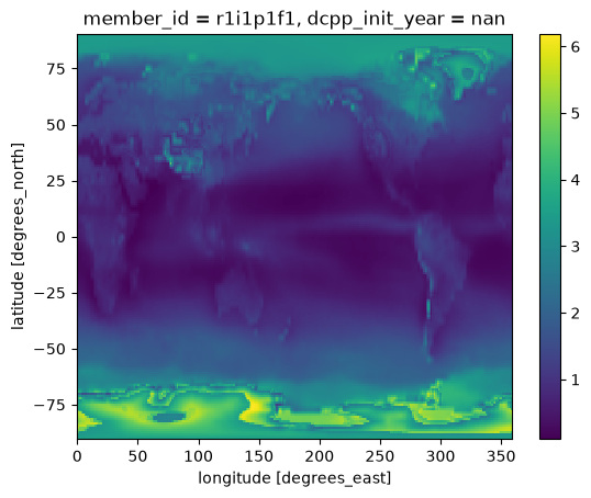
swq_feedback = dSW_q/dgmstswq_feedback.mean(dim='month').plot(cbar_kwargs={'label': 'W m$^{-2}$ K$^{-1}$'})Could not determine bucket type for bucket name cmip6: Your default credentials were not found. To set up Application Default Credentials, see https://cloud.google.com/docs/authentication/external/set-up-adc for more information., falling back to GCSFileSystem
Could not determine bucket type for bucket name cmip6: Your default credentials were not found. To set up Application Default Credentials, see https://cloud.google.com/docs/authentication/external/set-up-adc for more information., falling back to GCSFileSystem
Could not determine bucket type for bucket name cmip6: Your default credentials were not found. To set up Application Default Credentials, see https://cloud.google.com/docs/authentication/external/set-up-adc for more information., falling back to GCSFileSystem
Could not determine bucket type for bucket name cmip6: Your default credentials were not found. To set up Application Default Credentials, see https://cloud.google.com/docs/authentication/external/set-up-adc for more information., falling back to GCSFileSystem
Could not determine bucket type for bucket name cmip6: Your default credentials were not found. To set up Application Default Credentials, see https://cloud.google.com/docs/authentication/external/set-up-adc for more information., falling back to GCSFileSystem
Could not determine bucket type for bucket name cmip6: Your default credentials were not found. To set up Application Default Credentials, see https://cloud.google.com/docs/authentication/external/set-up-adc for more information., falling back to GCSFileSystem
Could not determine bucket type for bucket name cmip6: Your default credentials were not found. To set up Application Default Credentials, see https://cloud.google.com/docs/authentication/external/set-up-adc for more information., falling back to GCSFileSystem
Could not determine bucket type for bucket name cmip6: Your default credentials were not found. To set up Application Default Credentials, see https://cloud.google.com/docs/authentication/external/set-up-adc for more information., falling back to GCSFileSystem
Could not determine bucket type for bucket name cmip6: Your default credentials were not found. To set up Application Default Credentials, see https://cloud.google.com/docs/authentication/external/set-up-adc for more information., falling back to GCSFileSystem
Could not determine bucket type for bucket name cmip6: Your default credentials were not found. To set up Application Default Credentials, see https://cloud.google.com/docs/authentication/external/set-up-adc for more information., falling back to GCSFileSystem
Could not determine bucket type for bucket name cmip6: Your default credentials were not found. To set up Application Default Credentials, see https://cloud.google.com/docs/authentication/external/set-up-adc for more information., falling back to GCSFileSystem
Could not determine bucket type for bucket name cmip6: Your default credentials were not found. To set up Application Default Credentials, see https://cloud.google.com/docs/authentication/external/set-up-adc for more information., falling back to GCSFileSystem
Could not determine bucket type for bucket name cmip6: Your default credentials were not found. To set up Application Default Credentials, see https://cloud.google.com/docs/authentication/external/set-up-adc for more information., falling back to GCSFileSystem
Could not determine bucket type for bucket name cmip6: Your default credentials were not found. To set up Application Default Credentials, see https://cloud.google.com/docs/authentication/external/set-up-adc for more information., falling back to GCSFileSystem
Could not determine bucket type for bucket name cmip6: Your default credentials were not found. To set up Application Default Credentials, see https://cloud.google.com/docs/authentication/external/set-up-adc for more information., falling back to GCSFileSystem
Could not determine bucket type for bucket name cmip6: Your default credentials were not found. To set up Application Default Credentials, see https://cloud.google.com/docs/authentication/external/set-up-adc for more information., falling back to GCSFileSystem
Could not determine bucket type for bucket name cmip6: Your default credentials were not found. To set up Application Default Credentials, see https://cloud.google.com/docs/authentication/external/set-up-adc for more information., falling back to GCSFileSystem
Could not determine bucket type for bucket name cmip6: Your default credentials were not found. To set up Application Default Credentials, see https://cloud.google.com/docs/authentication/external/set-up-adc for more information., falling back to GCSFileSystem
Could not determine bucket type for bucket name cmip6: Your default credentials were not found. To set up Application Default Credentials, see https://cloud.google.com/docs/authentication/external/set-up-adc for more information., falling back to GCSFileSystem
Could not determine bucket type for bucket name cmip6: Your default credentials were not found. To set up Application Default Credentials, see https://cloud.google.com/docs/authentication/external/set-up-adc for more information., falling back to GCSFileSystem
Could not determine bucket type for bucket name cmip6: Your default credentials were not found. To set up Application Default Credentials, see https://cloud.google.com/docs/authentication/external/set-up-adc for more information., falling back to GCSFileSystem
Could not determine bucket type for bucket name cmip6: Your default credentials were not found. To set up Application Default Credentials, see https://cloud.google.com/docs/authentication/external/set-up-adc for more information., falling back to GCSFileSystem
Could not determine bucket type for bucket name cmip6: Your default credentials were not found. To set up Application Default Credentials, see https://cloud.google.com/docs/authentication/external/set-up-adc for more information., falling back to GCSFileSystem
Could not determine bucket type for bucket name cmip6: Your default credentials were not found. To set up Application Default Credentials, see https://cloud.google.com/docs/authentication/external/set-up-adc for more information., falling back to GCSFileSystem
Could not determine bucket type for bucket name cmip6: Your default credentials were not found. To set up Application Default Credentials, see https://cloud.google.com/docs/authentication/external/set-up-adc for more information., falling back to GCSFileSystem
Could not determine bucket type for bucket name cmip6: Your default credentials were not found. To set up Application Default Credentials, see https://cloud.google.com/docs/authentication/external/set-up-adc for more information., falling back to GCSFileSystem
Could not determine bucket type for bucket name cmip6: Your default credentials were not found. To set up Application Default Credentials, see https://cloud.google.com/docs/authentication/external/set-up-adc for more information., falling back to GCSFileSystem
Could not determine bucket type for bucket name cmip6: Your default credentials were not found. To set up Application Default Credentials, see https://cloud.google.com/docs/authentication/external/set-up-adc for more information., falling back to GCSFileSystem
Could not determine bucket type for bucket name cmip6: Your default credentials were not found. To set up Application Default Credentials, see https://cloud.google.com/docs/authentication/external/set-up-adc for more information., falling back to GCSFileSystem
Could not determine bucket type for bucket name cmip6: Your default credentials were not found. To set up Application Default Credentials, see https://cloud.google.com/docs/authentication/external/set-up-adc for more information., falling back to GCSFileSystem
Could not determine bucket type for bucket name cmip6: Your default credentials were not found. To set up Application Default Credentials, see https://cloud.google.com/docs/authentication/external/set-up-adc for more information., falling back to GCSFileSystem
Could not determine bucket type for bucket name cmip6: Your default credentials were not found. To set up Application Default Credentials, see https://cloud.google.com/docs/authentication/external/set-up-adc for more information., falling back to GCSFileSystem
Could not determine bucket type for bucket name cmip6: Your default credentials were not found. To set up Application Default Credentials, see https://cloud.google.com/docs/authentication/external/set-up-adc for more information., falling back to GCSFileSystem
Could not determine bucket type for bucket name cmip6: Your default credentials were not found. To set up Application Default Credentials, see https://cloud.google.com/docs/authentication/external/set-up-adc for more information., falling back to GCSFileSystem
Could not determine bucket type for bucket name cmip6: Your default credentials were not found. To set up Application Default Credentials, see https://cloud.google.com/docs/authentication/external/set-up-adc for more information., falling back to GCSFileSystem
Could not determine bucket type for bucket name cmip6: Your default credentials were not found. To set up Application Default Credentials, see https://cloud.google.com/docs/authentication/external/set-up-adc for more information., falling back to GCSFileSystem
Could not determine bucket type for bucket name cmip6: Your default credentials were not found. To set up Application Default Credentials, see https://cloud.google.com/docs/authentication/external/set-up-adc for more information., falling back to GCSFileSystem
Could not determine bucket type for bucket name cmip6: Your default credentials were not found. To set up Application Default Credentials, see https://cloud.google.com/docs/authentication/external/set-up-adc for more information., falling back to GCSFileSystem
Could not determine bucket type for bucket name cmip6: Your default credentials were not found. To set up Application Default Credentials, see https://cloud.google.com/docs/authentication/external/set-up-adc for more information., falling back to GCSFileSystem
Could not determine bucket type for bucket name cmip6: Your default credentials were not found. To set up Application Default Credentials, see https://cloud.google.com/docs/authentication/external/set-up-adc for more information., falling back to GCSFileSystem
Could not determine bucket type for bucket name cmip6: Your default credentials were not found. To set up Application Default Credentials, see https://cloud.google.com/docs/authentication/external/set-up-adc for more information., falling back to GCSFileSystem
Could not determine bucket type for bucket name cmip6: Your default credentials were not found. To set up Application Default Credentials, see https://cloud.google.com/docs/authentication/external/set-up-adc for more information., falling back to GCSFileSystem
Could not determine bucket type for bucket name cmip6: Your default credentials were not found. To set up Application Default Credentials, see https://cloud.google.com/docs/authentication/external/set-up-adc for more information., falling back to GCSFileSystem
Could not determine bucket type for bucket name cmip6: Your default credentials were not found. To set up Application Default Credentials, see https://cloud.google.com/docs/authentication/external/set-up-adc for more information., falling back to GCSFileSystem
Could not determine bucket type for bucket name cmip6: Your default credentials were not found. To set up Application Default Credentials, see https://cloud.google.com/docs/authentication/external/set-up-adc for more information., falling back to GCSFileSystem
Could not determine bucket type for bucket name cmip6: Your default credentials were not found. To set up Application Default Credentials, see https://cloud.google.com/docs/authentication/external/set-up-adc for more information., falling back to GCSFileSystem
Could not determine bucket type for bucket name cmip6: Your default credentials were not found. To set up Application Default Credentials, see https://cloud.google.com/docs/authentication/external/set-up-adc for more information., falling back to GCSFileSystem
Could not determine bucket type for bucket name cmip6: Your default credentials were not found. To set up Application Default Credentials, see https://cloud.google.com/docs/authentication/external/set-up-adc for more information., falling back to GCSFileSystem
Could not determine bucket type for bucket name cmip6: Your default credentials were not found. To set up Application Default Credentials, see https://cloud.google.com/docs/authentication/external/set-up-adc for more information., falling back to GCSFileSystem
Could not determine bucket type for bucket name cmip6: Your default credentials were not found. To set up Application Default Credentials, see https://cloud.google.com/docs/authentication/external/set-up-adc for more information., falling back to GCSFileSystem
Could not determine bucket type for bucket name cmip6: Your default credentials were not found. To set up Application Default Credentials, see https://cloud.google.com/docs/authentication/external/set-up-adc for more information., falling back to GCSFileSystem
Could not determine bucket type for bucket name cmip6: Your default credentials were not found. To set up Application Default Credentials, see https://cloud.google.com/docs/authentication/external/set-up-adc for more information., falling back to GCSFileSystem
Could not determine bucket type for bucket name cmip6: Your default credentials were not found. To set up Application Default Credentials, see https://cloud.google.com/docs/authentication/external/set-up-adc for more information., falling back to GCSFileSystem
Could not determine bucket type for bucket name cmip6: Your default credentials were not found. To set up Application Default Credentials, see https://cloud.google.com/docs/authentication/external/set-up-adc for more information., falling back to GCSFileSystem
Could not determine bucket type for bucket name cmip6: Your default credentials were not found. To set up Application Default Credentials, see https://cloud.google.com/docs/authentication/external/set-up-adc for more information., falling back to GCSFileSystem
Could not determine bucket type for bucket name cmip6: Your default credentials were not found. To set up Application Default Credentials, see https://cloud.google.com/docs/authentication/external/set-up-adc for more information., falling back to GCSFileSystem
Could not determine bucket type for bucket name cmip6: Your default credentials were not found. To set up Application Default Credentials, see https://cloud.google.com/docs/authentication/external/set-up-adc for more information., falling back to GCSFileSystem
Could not determine bucket type for bucket name cmip6: Your default credentials were not found. To set up Application Default Credentials, see https://cloud.google.com/docs/authentication/external/set-up-adc for more information., falling back to GCSFileSystem
Could not determine bucket type for bucket name cmip6: Your default credentials were not found. To set up Application Default Credentials, see https://cloud.google.com/docs/authentication/external/set-up-adc for more information., falling back to GCSFileSystem
Could not determine bucket type for bucket name cmip6: Your default credentials were not found. To set up Application Default Credentials, see https://cloud.google.com/docs/authentication/external/set-up-adc for more information., falling back to GCSFileSystem
Could not determine bucket type for bucket name cmip6: Your default credentials were not found. To set up Application Default Credentials, see https://cloud.google.com/docs/authentication/external/set-up-adc for more information., falling back to GCSFileSystem
Could not determine bucket type for bucket name cmip6: Your default credentials were not found. To set up Application Default Credentials, see https://cloud.google.com/docs/authentication/external/set-up-adc for more information., falling back to GCSFileSystem
Could not determine bucket type for bucket name cmip6: Your default credentials were not found. To set up Application Default Credentials, see https://cloud.google.com/docs/authentication/external/set-up-adc for more information., falling back to GCSFileSystem
Could not determine bucket type for bucket name cmip6: Your default credentials were not found. To set up Application Default Credentials, see https://cloud.google.com/docs/authentication/external/set-up-adc for more information., falling back to GCSFileSystem
Could not determine bucket type for bucket name cmip6: Your default credentials were not found. To set up Application Default Credentials, see https://cloud.google.com/docs/authentication/external/set-up-adc for more information., falling back to GCSFileSystem
Could not determine bucket type for bucket name cmip6: Your default credentials were not found. To set up Application Default Credentials, see https://cloud.google.com/docs/authentication/external/set-up-adc for more information., falling back to GCSFileSystem
Could not determine bucket type for bucket name cmip6: Your default credentials were not found. To set up Application Default Credentials, see https://cloud.google.com/docs/authentication/external/set-up-adc for more information., falling back to GCSFileSystem
Could not determine bucket type for bucket name cmip6: Your default credentials were not found. To set up Application Default Credentials, see https://cloud.google.com/docs/authentication/external/set-up-adc for more information., falling back to GCSFileSystem
Could not determine bucket type for bucket name cmip6: Your default credentials were not found. To set up Application Default Credentials, see https://cloud.google.com/docs/authentication/external/set-up-adc for more information., falling back to GCSFileSystem
Could not determine bucket type for bucket name cmip6: Your default credentials were not found. To set up Application Default Credentials, see https://cloud.google.com/docs/authentication/external/set-up-adc for more information., falling back to GCSFileSystem
Could not determine bucket type for bucket name cmip6: Your default credentials were not found. To set up Application Default Credentials, see https://cloud.google.com/docs/authentication/external/set-up-adc for more information., falling back to GCSFileSystem
Could not determine bucket type for bucket name cmip6: Your default credentials were not found. To set up Application Default Credentials, see https://cloud.google.com/docs/authentication/external/set-up-adc for more information., falling back to GCSFileSystem
Could not determine bucket type for bucket name cmip6: Your default credentials were not found. To set up Application Default Credentials, see https://cloud.google.com/docs/authentication/external/set-up-adc for more information., falling back to GCSFileSystem
Could not determine bucket type for bucket name cmip6: Your default credentials were not found. To set up Application Default Credentials, see https://cloud.google.com/docs/authentication/external/set-up-adc for more information., falling back to GCSFileSystem
Could not determine bucket type for bucket name cmip6: Your default credentials were not found. To set up Application Default Credentials, see https://cloud.google.com/docs/authentication/external/set-up-adc for more information., falling back to GCSFileSystem
Could not determine bucket type for bucket name cmip6: Your default credentials were not found. To set up Application Default Credentials, see https://cloud.google.com/docs/authentication/external/set-up-adc for more information., falling back to GCSFileSystem
Could not determine bucket type for bucket name cmip6: Your default credentials were not found. To set up Application Default Credentials, see https://cloud.google.com/docs/authentication/external/set-up-adc for more information., falling back to GCSFileSystem
Could not determine bucket type for bucket name cmip6: Your default credentials were not found. To set up Application Default Credentials, see https://cloud.google.com/docs/authentication/external/set-up-adc for more information., falling back to GCSFileSystem
Could not determine bucket type for bucket name cmip6: Your default credentials were not found. To set up Application Default Credentials, see https://cloud.google.com/docs/authentication/external/set-up-adc for more information., falling back to GCSFileSystem
Could not determine bucket type for bucket name cmip6: Your default credentials were not found. To set up Application Default Credentials, see https://cloud.google.com/docs/authentication/external/set-up-adc for more information., falling back to GCSFileSystem
Could not determine bucket type for bucket name cmip6: Your default credentials were not found. To set up Application Default Credentials, see https://cloud.google.com/docs/authentication/external/set-up-adc for more information., falling back to GCSFileSystem
Could not determine bucket type for bucket name cmip6: Your default credentials were not found. To set up Application Default Credentials, see https://cloud.google.com/docs/authentication/external/set-up-adc for more information., falling back to GCSFileSystem
Could not determine bucket type for bucket name cmip6: Your default credentials were not found. To set up Application Default Credentials, see https://cloud.google.com/docs/authentication/external/set-up-adc for more information., falling back to GCSFileSystem
Could not determine bucket type for bucket name cmip6: Your default credentials were not found. To set up Application Default Credentials, see https://cloud.google.com/docs/authentication/external/set-up-adc for more information., falling back to GCSFileSystem
Could not determine bucket type for bucket name cmip6: Your default credentials were not found. To set up Application Default Credentials, see https://cloud.google.com/docs/authentication/external/set-up-adc for more information., falling back to GCSFileSystem
Could not determine bucket type for bucket name cmip6: Your default credentials were not found. To set up Application Default Credentials, see https://cloud.google.com/docs/authentication/external/set-up-adc for more information., falling back to GCSFileSystem
Could not determine bucket type for bucket name cmip6: Your default credentials were not found. To set up Application Default Credentials, see https://cloud.google.com/docs/authentication/external/set-up-adc for more information., falling back to GCSFileSystem
Could not determine bucket type for bucket name cmip6: Your default credentials were not found. To set up Application Default Credentials, see https://cloud.google.com/docs/authentication/external/set-up-adc for more information., falling back to GCSFileSystem
Could not determine bucket type for bucket name cmip6: Your default credentials were not found. To set up Application Default Credentials, see https://cloud.google.com/docs/authentication/external/set-up-adc for more information., falling back to GCSFileSystem
Could not determine bucket type for bucket name cmip6: Your default credentials were not found. To set up Application Default Credentials, see https://cloud.google.com/docs/authentication/external/set-up-adc for more information., falling back to GCSFileSystem
Could not determine bucket type for bucket name cmip6: Your default credentials were not found. To set up Application Default Credentials, see https://cloud.google.com/docs/authentication/external/set-up-adc for more information., falling back to GCSFileSystem
Could not determine bucket type for bucket name cmip6: Your default credentials were not found. To set up Application Default Credentials, see https://cloud.google.com/docs/authentication/external/set-up-adc for more information., falling back to GCSFileSystem
Could not determine bucket type for bucket name cmip6: Your default credentials were not found. To set up Application Default Credentials, see https://cloud.google.com/docs/authentication/external/set-up-adc for more information., falling back to GCSFileSystem
Could not determine bucket type for bucket name cmip6: Your default credentials were not found. To set up Application Default Credentials, see https://cloud.google.com/docs/authentication/external/set-up-adc for more information., falling back to GCSFileSystem
Could not determine bucket type for bucket name cmip6: Your default credentials were not found. To set up Application Default Credentials, see https://cloud.google.com/docs/authentication/external/set-up-adc for more information., falling back to GCSFileSystem
Could not determine bucket type for bucket name cmip6: Your default credentials were not found. To set up Application Default Credentials, see https://cloud.google.com/docs/authentication/external/set-up-adc for more information., falling back to GCSFileSystem
Could not determine bucket type for bucket name cmip6: Your default credentials were not found. To set up Application Default Credentials, see https://cloud.google.com/docs/authentication/external/set-up-adc for more information., falling back to GCSFileSystem
Could not determine bucket type for bucket name cmip6: Your default credentials were not found. To set up Application Default Credentials, see https://cloud.google.com/docs/authentication/external/set-up-adc for more information., falling back to GCSFileSystem
Could not determine bucket type for bucket name cmip6: Your default credentials were not found. To set up Application Default Credentials, see https://cloud.google.com/docs/authentication/external/set-up-adc for more information., falling back to GCSFileSystem
Could not determine bucket type for bucket name cmip6: Your default credentials were not found. To set up Application Default Credentials, see https://cloud.google.com/docs/authentication/external/set-up-adc for more information., falling back to GCSFileSystem
Could not determine bucket type for bucket name cmip6: Your default credentials were not found. To set up Application Default Credentials, see https://cloud.google.com/docs/authentication/external/set-up-adc for more information., falling back to GCSFileSystem
Could not determine bucket type for bucket name cmip6: Your default credentials were not found. To set up Application Default Credentials, see https://cloud.google.com/docs/authentication/external/set-up-adc for more information., falling back to GCSFileSystem
Could not determine bucket type for bucket name cmip6: Your default credentials were not found. To set up Application Default Credentials, see https://cloud.google.com/docs/authentication/external/set-up-adc for more information., falling back to GCSFileSystem
Could not determine bucket type for bucket name cmip6: Your default credentials were not found. To set up Application Default Credentials, see https://cloud.google.com/docs/authentication/external/set-up-adc for more information., falling back to GCSFileSystem
Could not determine bucket type for bucket name cmip6: Your default credentials were not found. To set up Application Default Credentials, see https://cloud.google.com/docs/authentication/external/set-up-adc for more information., falling back to GCSFileSystem
Could not determine bucket type for bucket name cmip6: Your default credentials were not found. To set up Application Default Credentials, see https://cloud.google.com/docs/authentication/external/set-up-adc for more information., falling back to GCSFileSystem
Could not determine bucket type for bucket name cmip6: Your default credentials were not found. To set up Application Default Credentials, see https://cloud.google.com/docs/authentication/external/set-up-adc for more information., falling back to GCSFileSystem
Could not determine bucket type for bucket name cmip6: Your default credentials were not found. To set up Application Default Credentials, see https://cloud.google.com/docs/authentication/external/set-up-adc for more information., falling back to GCSFileSystem
Could not determine bucket type for bucket name cmip6: Your default credentials were not found. To set up Application Default Credentials, see https://cloud.google.com/docs/authentication/external/set-up-adc for more information., falling back to GCSFileSystem
Could not determine bucket type for bucket name cmip6: Your default credentials were not found. To set up Application Default Credentials, see https://cloud.google.com/docs/authentication/external/set-up-adc for more information., falling back to GCSFileSystem
Could not determine bucket type for bucket name cmip6: Your default credentials were not found. To set up Application Default Credentials, see https://cloud.google.com/docs/authentication/external/set-up-adc for more information., falling back to GCSFileSystem
Could not determine bucket type for bucket name cmip6: Your default credentials were not found. To set up Application Default Credentials, see https://cloud.google.com/docs/authentication/external/set-up-adc for more information., falling back to GCSFileSystem
Could not determine bucket type for bucket name cmip6: Your default credentials were not found. To set up Application Default Credentials, see https://cloud.google.com/docs/authentication/external/set-up-adc for more information., falling back to GCSFileSystem
Could not determine bucket type for bucket name cmip6: Your default credentials were not found. To set up Application Default Credentials, see https://cloud.google.com/docs/authentication/external/set-up-adc for more information., falling back to GCSFileSystem
Could not determine bucket type for bucket name cmip6: Your default credentials were not found. To set up Application Default Credentials, see https://cloud.google.com/docs/authentication/external/set-up-adc for more information., falling back to GCSFileSystem
Could not determine bucket type for bucket name cmip6: Your default credentials were not found. To set up Application Default Credentials, see https://cloud.google.com/docs/authentication/external/set-up-adc for more information., falling back to GCSFileSystem
Could not determine bucket type for bucket name cmip6: Your default credentials were not found. To set up Application Default Credentials, see https://cloud.google.com/docs/authentication/external/set-up-adc for more information., falling back to GCSFileSystem
Could not determine bucket type for bucket name cmip6: Your default credentials were not found. To set up Application Default Credentials, see https://cloud.google.com/docs/authentication/external/set-up-adc for more information., falling back to GCSFileSystem
Could not determine bucket type for bucket name cmip6: Your default credentials were not found. To set up Application Default Credentials, see https://cloud.google.com/docs/authentication/external/set-up-adc for more information., falling back to GCSFileSystem
Could not determine bucket type for bucket name cmip6: Your default credentials were not found. To set up Application Default Credentials, see https://cloud.google.com/docs/authentication/external/set-up-adc for more information., falling back to GCSFileSystem
Could not determine bucket type for bucket name cmip6: Your default credentials were not found. To set up Application Default Credentials, see https://cloud.google.com/docs/authentication/external/set-up-adc for more information., falling back to GCSFileSystem
Could not determine bucket type for bucket name cmip6: Your default credentials were not found. To set up Application Default Credentials, see https://cloud.google.com/docs/authentication/external/set-up-adc for more information., falling back to GCSFileSystem
Could not determine bucket type for bucket name cmip6: Your default credentials were not found. To set up Application Default Credentials, see https://cloud.google.com/docs/authentication/external/set-up-adc for more information., falling back to GCSFileSystem
Could not determine bucket type for bucket name cmip6: Your default credentials were not found. To set up Application Default Credentials, see https://cloud.google.com/docs/authentication/external/set-up-adc for more information., falling back to GCSFileSystem
Could not determine bucket type for bucket name cmip6: Your default credentials were not found. To set up Application Default Credentials, see https://cloud.google.com/docs/authentication/external/set-up-adc for more information., falling back to GCSFileSystem
Could not determine bucket type for bucket name cmip6: Your default credentials were not found. To set up Application Default Credentials, see https://cloud.google.com/docs/authentication/external/set-up-adc for more information., falling back to GCSFileSystem
Could not determine bucket type for bucket name cmip6: Your default credentials were not found. To set up Application Default Credentials, see https://cloud.google.com/docs/authentication/external/set-up-adc for more information., falling back to GCSFileSystem
Could not determine bucket type for bucket name cmip6: Your default credentials were not found. To set up Application Default Credentials, see https://cloud.google.com/docs/authentication/external/set-up-adc for more information., falling back to GCSFileSystem
Could not determine bucket type for bucket name cmip6: Your default credentials were not found. To set up Application Default Credentials, see https://cloud.google.com/docs/authentication/external/set-up-adc for more information., falling back to GCSFileSystem
Could not determine bucket type for bucket name cmip6: Your default credentials were not found. To set up Application Default Credentials, see https://cloud.google.com/docs/authentication/external/set-up-adc for more information., falling back to GCSFileSystem
Could not determine bucket type for bucket name cmip6: Your default credentials were not found. To set up Application Default Credentials, see https://cloud.google.com/docs/authentication/external/set-up-adc for more information., falling back to GCSFileSystem
Could not determine bucket type for bucket name cmip6: Your default credentials were not found. To set up Application Default Credentials, see https://cloud.google.com/docs/authentication/external/set-up-adc for more information., falling back to GCSFileSystem
Could not determine bucket type for bucket name cmip6: Your default credentials were not found. To set up Application Default Credentials, see https://cloud.google.com/docs/authentication/external/set-up-adc for more information., falling back to GCSFileSystem
Could not determine bucket type for bucket name cmip6: Your default credentials were not found. To set up Application Default Credentials, see https://cloud.google.com/docs/authentication/external/set-up-adc for more information., falling back to GCSFileSystem
Could not determine bucket type for bucket name cmip6: Your default credentials were not found. To set up Application Default Credentials, see https://cloud.google.com/docs/authentication/external/set-up-adc for more information., falling back to GCSFileSystem
Could not determine bucket type for bucket name cmip6: Your default credentials were not found. To set up Application Default Credentials, see https://cloud.google.com/docs/authentication/external/set-up-adc for more information., falling back to GCSFileSystem
Could not determine bucket type for bucket name cmip6: Your default credentials were not found. To set up Application Default Credentials, see https://cloud.google.com/docs/authentication/external/set-up-adc for more information., falling back to GCSFileSystem
Could not determine bucket type for bucket name cmip6: Your default credentials were not found. To set up Application Default Credentials, see https://cloud.google.com/docs/authentication/external/set-up-adc for more information., falling back to GCSFileSystem
Could not determine bucket type for bucket name cmip6: Your default credentials were not found. To set up Application Default Credentials, see https://cloud.google.com/docs/authentication/external/set-up-adc for more information., falling back to GCSFileSystem
Could not determine bucket type for bucket name cmip6: Your default credentials were not found. To set up Application Default Credentials, see https://cloud.google.com/docs/authentication/external/set-up-adc for more information., falling back to GCSFileSystem
Could not determine bucket type for bucket name cmip6: Your default credentials were not found. To set up Application Default Credentials, see https://cloud.google.com/docs/authentication/external/set-up-adc for more information., falling back to GCSFileSystem
Could not determine bucket type for bucket name cmip6: Your default credentials were not found. To set up Application Default Credentials, see https://cloud.google.com/docs/authentication/external/set-up-adc for more information., falling back to GCSFileSystem
Could not determine bucket type for bucket name cmip6: Your default credentials were not found. To set up Application Default Credentials, see https://cloud.google.com/docs/authentication/external/set-up-adc for more information., falling back to GCSFileSystem
Could not determine bucket type for bucket name cmip6: Your default credentials were not found. To set up Application Default Credentials, see https://cloud.google.com/docs/authentication/external/set-up-adc for more information., falling back to GCSFileSystem
Could not determine bucket type for bucket name cmip6: Your default credentials were not found. To set up Application Default Credentials, see https://cloud.google.com/docs/authentication/external/set-up-adc for more information., falling back to GCSFileSystem
Could not determine bucket type for bucket name cmip6: Your default credentials were not found. To set up Application Default Credentials, see https://cloud.google.com/docs/authentication/external/set-up-adc for more information., falling back to GCSFileSystem
Could not determine bucket type for bucket name cmip6: Your default credentials were not found. To set up Application Default Credentials, see https://cloud.google.com/docs/authentication/external/set-up-adc for more information., falling back to GCSFileSystem
Could not determine bucket type for bucket name cmip6: Your default credentials were not found. To set up Application Default Credentials, see https://cloud.google.com/docs/authentication/external/set-up-adc for more information., falling back to GCSFileSystem
Could not determine bucket type for bucket name cmip6: Your default credentials were not found. To set up Application Default Credentials, see https://cloud.google.com/docs/authentication/external/set-up-adc for more information., falling back to GCSFileSystem
Could not determine bucket type for bucket name cmip6: Your default credentials were not found. To set up Application Default Credentials, see https://cloud.google.com/docs/authentication/external/set-up-adc for more information., falling back to GCSFileSystem
Could not determine bucket type for bucket name cmip6: Your default credentials were not found. To set up Application Default Credentials, see https://cloud.google.com/docs/authentication/external/set-up-adc for more information., falling back to GCSFileSystem
Could not determine bucket type for bucket name cmip6: Your default credentials were not found. To set up Application Default Credentials, see https://cloud.google.com/docs/authentication/external/set-up-adc for more information., falling back to GCSFileSystem
Could not determine bucket type for bucket name cmip6: Your default credentials were not found. To set up Application Default Credentials, see https://cloud.google.com/docs/authentication/external/set-up-adc for more information., falling back to GCSFileSystem
Could not determine bucket type for bucket name cmip6: Your default credentials were not found. To set up Application Default Credentials, see https://cloud.google.com/docs/authentication/external/set-up-adc for more information., falling back to GCSFileSystem
Could not determine bucket type for bucket name cmip6: Your default credentials were not found. To set up Application Default Credentials, see https://cloud.google.com/docs/authentication/external/set-up-adc for more information., falling back to GCSFileSystem
Could not determine bucket type for bucket name cmip6: Your default credentials were not found. To set up Application Default Credentials, see https://cloud.google.com/docs/authentication/external/set-up-adc for more information., falling back to GCSFileSystem
Could not determine bucket type for bucket name cmip6: Your default credentials were not found. To set up Application Default Credentials, see https://cloud.google.com/docs/authentication/external/set-up-adc for more information., falling back to GCSFileSystem
Could not determine bucket type for bucket name cmip6: Your default credentials were not found. To set up Application Default Credentials, see https://cloud.google.com/docs/authentication/external/set-up-adc for more information., falling back to GCSFileSystem
Could not determine bucket type for bucket name cmip6: Your default credentials were not found. To set up Application Default Credentials, see https://cloud.google.com/docs/authentication/external/set-up-adc for more information., falling back to GCSFileSystem
Could not determine bucket type for bucket name cmip6: Your default credentials were not found. To set up Application Default Credentials, see https://cloud.google.com/docs/authentication/external/set-up-adc for more information., falling back to GCSFileSystem
Could not determine bucket type for bucket name cmip6: Your default credentials were not found. To set up Application Default Credentials, see https://cloud.google.com/docs/authentication/external/set-up-adc for more information., falling back to GCSFileSystem
Could not determine bucket type for bucket name cmip6: Your default credentials were not found. To set up Application Default Credentials, see https://cloud.google.com/docs/authentication/external/set-up-adc for more information., falling back to GCSFileSystem
Could not determine bucket type for bucket name cmip6: Your default credentials were not found. To set up Application Default Credentials, see https://cloud.google.com/docs/authentication/external/set-up-adc for more information., falling back to GCSFileSystem
Could not determine bucket type for bucket name cmip6: Your default credentials were not found. To set up Application Default Credentials, see https://cloud.google.com/docs/authentication/external/set-up-adc for more information., falling back to GCSFileSystem
Could not determine bucket type for bucket name cmip6: Your default credentials were not found. To set up Application Default Credentials, see https://cloud.google.com/docs/authentication/external/set-up-adc for more information., falling back to GCSFileSystem
Could not determine bucket type for bucket name cmip6: Your default credentials were not found. To set up Application Default Credentials, see https://cloud.google.com/docs/authentication/external/set-up-adc for more information., falling back to GCSFileSystem
Could not determine bucket type for bucket name cmip6: Your default credentials were not found. To set up Application Default Credentials, see https://cloud.google.com/docs/authentication/external/set-up-adc for more information., falling back to GCSFileSystem
Could not determine bucket type for bucket name cmip6: Your default credentials were not found. To set up Application Default Credentials, see https://cloud.google.com/docs/authentication/external/set-up-adc for more information., falling back to GCSFileSystem
Could not determine bucket type for bucket name cmip6: Your default credentials were not found. To set up Application Default Credentials, see https://cloud.google.com/docs/authentication/external/set-up-adc for more information., falling back to GCSFileSystem
Could not determine bucket type for bucket name cmip6: Your default credentials were not found. To set up Application Default Credentials, see https://cloud.google.com/docs/authentication/external/set-up-adc for more information., falling back to GCSFileSystem
Could not determine bucket type for bucket name cmip6: Your default credentials were not found. To set up Application Default Credentials, see https://cloud.google.com/docs/authentication/external/set-up-adc for more information., falling back to GCSFileSystem
Could not determine bucket type for bucket name cmip6: Your default credentials were not found. To set up Application Default Credentials, see https://cloud.google.com/docs/authentication/external/set-up-adc for more information., falling back to GCSFileSystem
Could not determine bucket type for bucket name cmip6: Your default credentials were not found. To set up Application Default Credentials, see https://cloud.google.com/docs/authentication/external/set-up-adc for more information., falling back to GCSFileSystem
Could not determine bucket type for bucket name cmip6: Your default credentials were not found. To set up Application Default Credentials, see https://cloud.google.com/docs/authentication/external/set-up-adc for more information., falling back to GCSFileSystem
Could not determine bucket type for bucket name cmip6: Your default credentials were not found. To set up Application Default Credentials, see https://cloud.google.com/docs/authentication/external/set-up-adc for more information., falling back to GCSFileSystem
Could not determine bucket type for bucket name cmip6: Your default credentials were not found. To set up Application Default Credentials, see https://cloud.google.com/docs/authentication/external/set-up-adc for more information., falling back to GCSFileSystem
Could not determine bucket type for bucket name cmip6: Your default credentials were not found. To set up Application Default Credentials, see https://cloud.google.com/docs/authentication/external/set-up-adc for more information., falling back to GCSFileSystem
Could not determine bucket type for bucket name cmip6: Your default credentials were not found. To set up Application Default Credentials, see https://cloud.google.com/docs/authentication/external/set-up-adc for more information., falling back to GCSFileSystem
Could not determine bucket type for bucket name cmip6: Your default credentials were not found. To set up Application Default Credentials, see https://cloud.google.com/docs/authentication/external/set-up-adc for more information., falling back to GCSFileSystem
Could not determine bucket type for bucket name cmip6: Your default credentials were not found. To set up Application Default Credentials, see https://cloud.google.com/docs/authentication/external/set-up-adc for more information., falling back to GCSFileSystem
Could not determine bucket type for bucket name cmip6: Your default credentials were not found. To set up Application Default Credentials, see https://cloud.google.com/docs/authentication/external/set-up-adc for more information., falling back to GCSFileSystem
Could not determine bucket type for bucket name cmip6: Your default credentials were not found. To set up Application Default Credentials, see https://cloud.google.com/docs/authentication/external/set-up-adc for more information., falling back to GCSFileSystem
Could not determine bucket type for bucket name cmip6: Your default credentials were not found. To set up Application Default Credentials, see https://cloud.google.com/docs/authentication/external/set-up-adc for more information., falling back to GCSFileSystem
Could not determine bucket type for bucket name cmip6: Your default credentials were not found. To set up Application Default Credentials, see https://cloud.google.com/docs/authentication/external/set-up-adc for more information., falling back to GCSFileSystem
Could not determine bucket type for bucket name cmip6: Your default credentials were not found. To set up Application Default Credentials, see https://cloud.google.com/docs/authentication/external/set-up-adc for more information., falling back to GCSFileSystem
Could not determine bucket type for bucket name cmip6: Your default credentials were not found. To set up Application Default Credentials, see https://cloud.google.com/docs/authentication/external/set-up-adc for more information., falling back to GCSFileSystem
Could not determine bucket type for bucket name cmip6: Your default credentials were not found. To set up Application Default Credentials, see https://cloud.google.com/docs/authentication/external/set-up-adc for more information., falling back to GCSFileSystem
Could not determine bucket type for bucket name cmip6: Your default credentials were not found. To set up Application Default Credentials, see https://cloud.google.com/docs/authentication/external/set-up-adc for more information., falling back to GCSFileSystem
Could not determine bucket type for bucket name cmip6: Your default credentials were not found. To set up Application Default Credentials, see https://cloud.google.com/docs/authentication/external/set-up-adc for more information., falling back to GCSFileSystem
Could not determine bucket type for bucket name cmip6: Your default credentials were not found. To set up Application Default Credentials, see https://cloud.google.com/docs/authentication/external/set-up-adc for more information., falling back to GCSFileSystem
Could not determine bucket type for bucket name cmip6: Your default credentials were not found. To set up Application Default Credentials, see https://cloud.google.com/docs/authentication/external/set-up-adc for more information., falling back to GCSFileSystem
Could not determine bucket type for bucket name cmip6: Your default credentials were not found. To set up Application Default Credentials, see https://cloud.google.com/docs/authentication/external/set-up-adc for more information., falling back to GCSFileSystem
Could not determine bucket type for bucket name cmip6: Your default credentials were not found. To set up Application Default Credentials, see https://cloud.google.com/docs/authentication/external/set-up-adc for more information., falling back to GCSFileSystem
Could not determine bucket type for bucket name cmip6: Your default credentials were not found. To set up Application Default Credentials, see https://cloud.google.com/docs/authentication/external/set-up-adc for more information., falling back to GCSFileSystem
Could not determine bucket type for bucket name cmip6: Your default credentials were not found. To set up Application Default Credentials, see https://cloud.google.com/docs/authentication/external/set-up-adc for more information., falling back to GCSFileSystem
Could not determine bucket type for bucket name cmip6: Your default credentials were not found. To set up Application Default Credentials, see https://cloud.google.com/docs/authentication/external/set-up-adc for more information., falling back to GCSFileSystem
Could not determine bucket type for bucket name cmip6: Your default credentials were not found. To set up Application Default Credentials, see https://cloud.google.com/docs/authentication/external/set-up-adc for more information., falling back to GCSFileSystem
Could not determine bucket type for bucket name cmip6: Your default credentials were not found. To set up Application Default Credentials, see https://cloud.google.com/docs/authentication/external/set-up-adc for more information., falling back to GCSFileSystem
Could not determine bucket type for bucket name cmip6: Your default credentials were not found. To set up Application Default Credentials, see https://cloud.google.com/docs/authentication/external/set-up-adc for more information., falling back to GCSFileSystem
Could not determine bucket type for bucket name cmip6: Your default credentials were not found. To set up Application Default Credentials, see https://cloud.google.com/docs/authentication/external/set-up-adc for more information., falling back to GCSFileSystem
Could not determine bucket type for bucket name cmip6: Your default credentials were not found. To set up Application Default Credentials, see https://cloud.google.com/docs/authentication/external/set-up-adc for more information., falling back to GCSFileSystem
Could not determine bucket type for bucket name cmip6: Your default credentials were not found. To set up Application Default Credentials, see https://cloud.google.com/docs/authentication/external/set-up-adc for more information., falling back to GCSFileSystem
Could not determine bucket type for bucket name cmip6: Your default credentials were not found. To set up Application Default Credentials, see https://cloud.google.com/docs/authentication/external/set-up-adc for more information., falling back to GCSFileSystem
Could not determine bucket type for bucket name cmip6: Your default credentials were not found. To set up Application Default Credentials, see https://cloud.google.com/docs/authentication/external/set-up-adc for more information., falling back to GCSFileSystem
Could not determine bucket type for bucket name cmip6: Your default credentials were not found. To set up Application Default Credentials, see https://cloud.google.com/docs/authentication/external/set-up-adc for more information., falling back to GCSFileSystem
Could not determine bucket type for bucket name cmip6: Your default credentials were not found. To set up Application Default Credentials, see https://cloud.google.com/docs/authentication/external/set-up-adc for more information., falling back to GCSFileSystem
Could not determine bucket type for bucket name cmip6: Your default credentials were not found. To set up Application Default Credentials, see https://cloud.google.com/docs/authentication/external/set-up-adc for more information., falling back to GCSFileSystem
Could not determine bucket type for bucket name cmip6: Your default credentials were not found. To set up Application Default Credentials, see https://cloud.google.com/docs/authentication/external/set-up-adc for more information., falling back to GCSFileSystem
Could not determine bucket type for bucket name cmip6: Your default credentials were not found. To set up Application Default Credentials, see https://cloud.google.com/docs/authentication/external/set-up-adc for more information., falling back to GCSFileSystem
Could not determine bucket type for bucket name cmip6: Your default credentials were not found. To set up Application Default Credentials, see https://cloud.google.com/docs/authentication/external/set-up-adc for more information., falling back to GCSFileSystem
Could not determine bucket type for bucket name cmip6: Your default credentials were not found. To set up Application Default Credentials, see https://cloud.google.com/docs/authentication/external/set-up-adc for more information., falling back to GCSFileSystem
Could not determine bucket type for bucket name cmip6: Your default credentials were not found. To set up Application Default Credentials, see https://cloud.google.com/docs/authentication/external/set-up-adc for more information., falling back to GCSFileSystem
Could not determine bucket type for bucket name cmip6: Your default credentials were not found. To set up Application Default Credentials, see https://cloud.google.com/docs/authentication/external/set-up-adc for more information., falling back to GCSFileSystem
Could not determine bucket type for bucket name cmip6: Your default credentials were not found. To set up Application Default Credentials, see https://cloud.google.com/docs/authentication/external/set-up-adc for more information., falling back to GCSFileSystem
Could not determine bucket type for bucket name cmip6: Your default credentials were not found. To set up Application Default Credentials, see https://cloud.google.com/docs/authentication/external/set-up-adc for more information., falling back to GCSFileSystem
Could not determine bucket type for bucket name cmip6: Your default credentials were not found. To set up Application Default Credentials, see https://cloud.google.com/docs/authentication/external/set-up-adc for more information., falling back to GCSFileSystem
Could not determine bucket type for bucket name cmip6: Your default credentials were not found. To set up Application Default Credentials, see https://cloud.google.com/docs/authentication/external/set-up-adc for more information., falling back to GCSFileSystem
Could not determine bucket type for bucket name cmip6: Your default credentials were not found. To set up Application Default Credentials, see https://cloud.google.com/docs/authentication/external/set-up-adc for more information., falling back to GCSFileSystem
Could not determine bucket type for bucket name cmip6: Your default credentials were not found. To set up Application Default Credentials, see https://cloud.google.com/docs/authentication/external/set-up-adc for more information., falling back to GCSFileSystem
Could not determine bucket type for bucket name cmip6: Your default credentials were not found. To set up Application Default Credentials, see https://cloud.google.com/docs/authentication/external/set-up-adc for more information., falling back to GCSFileSystem
Could not determine bucket type for bucket name cmip6: Your default credentials were not found. To set up Application Default Credentials, see https://cloud.google.com/docs/authentication/external/set-up-adc for more information., falling back to GCSFileSystem
Could not determine bucket type for bucket name cmip6: Your default credentials were not found. To set up Application Default Credentials, see https://cloud.google.com/docs/authentication/external/set-up-adc for more information., falling back to GCSFileSystem
Could not determine bucket type for bucket name cmip6: Your default credentials were not found. To set up Application Default Credentials, see https://cloud.google.com/docs/authentication/external/set-up-adc for more information., falling back to GCSFileSystem
Could not determine bucket type for bucket name cmip6: Your default credentials were not found. To set up Application Default Credentials, see https://cloud.google.com/docs/authentication/external/set-up-adc for more information., falling back to GCSFileSystem
Could not determine bucket type for bucket name cmip6: Your default credentials were not found. To set up Application Default Credentials, see https://cloud.google.com/docs/authentication/external/set-up-adc for more information., falling back to GCSFileSystem
Could not determine bucket type for bucket name cmip6: Your default credentials were not found. To set up Application Default Credentials, see https://cloud.google.com/docs/authentication/external/set-up-adc for more information., falling back to GCSFileSystem
Could not determine bucket type for bucket name cmip6: Your default credentials were not found. To set up Application Default Credentials, see https://cloud.google.com/docs/authentication/external/set-up-adc for more information., falling back to GCSFileSystem
Could not determine bucket type for bucket name cmip6: Your default credentials were not found. To set up Application Default Credentials, see https://cloud.google.com/docs/authentication/external/set-up-adc for more information., falling back to GCSFileSystem
Could not determine bucket type for bucket name cmip6: Your default credentials were not found. To set up Application Default Credentials, see https://cloud.google.com/docs/authentication/external/set-up-adc for more information., falling back to GCSFileSystem
Could not determine bucket type for bucket name cmip6: Your default credentials were not found. To set up Application Default Credentials, see https://cloud.google.com/docs/authentication/external/set-up-adc for more information., falling back to GCSFileSystem
Could not determine bucket type for bucket name cmip6: Your default credentials were not found. To set up Application Default Credentials, see https://cloud.google.com/docs/authentication/external/set-up-adc for more information., falling back to GCSFileSystem
Could not determine bucket type for bucket name cmip6: Your default credentials were not found. To set up Application Default Credentials, see https://cloud.google.com/docs/authentication/external/set-up-adc for more information., falling back to GCSFileSystem
Could not determine bucket type for bucket name cmip6: Your default credentials were not found. To set up Application Default Credentials, see https://cloud.google.com/docs/authentication/external/set-up-adc for more information., falling back to GCSFileSystem
Could not determine bucket type for bucket name cmip6: Your default credentials were not found. To set up Application Default Credentials, see https://cloud.google.com/docs/authentication/external/set-up-adc for more information., falling back to GCSFileSystem
Could not determine bucket type for bucket name cmip6: Your default credentials were not found. To set up Application Default Credentials, see https://cloud.google.com/docs/authentication/external/set-up-adc for more information., falling back to GCSFileSystem
Could not determine bucket type for bucket name cmip6: Your default credentials were not found. To set up Application Default Credentials, see https://cloud.google.com/docs/authentication/external/set-up-adc for more information., falling back to GCSFileSystem
Could not determine bucket type for bucket name cmip6: Your default credentials were not found. To set up Application Default Credentials, see https://cloud.google.com/docs/authentication/external/set-up-adc for more information., falling back to GCSFileSystem
Could not determine bucket type for bucket name cmip6: Your default credentials were not found. To set up Application Default Credentials, see https://cloud.google.com/docs/authentication/external/set-up-adc for more information., falling back to GCSFileSystem
Could not determine bucket type for bucket name cmip6: Your default credentials were not found. To set up Application Default Credentials, see https://cloud.google.com/docs/authentication/external/set-up-adc for more information., falling back to GCSFileSystem
Could not determine bucket type for bucket name cmip6: Your default credentials were not found. To set up Application Default Credentials, see https://cloud.google.com/docs/authentication/external/set-up-adc for more information., falling back to GCSFileSystem
Could not determine bucket type for bucket name cmip6: Your default credentials were not found. To set up Application Default Credentials, see https://cloud.google.com/docs/authentication/external/set-up-adc for more information., falling back to GCSFileSystem
Could not determine bucket type for bucket name cmip6: Your default credentials were not found. To set up Application Default Credentials, see https://cloud.google.com/docs/authentication/external/set-up-adc for more information., falling back to GCSFileSystem
Could not determine bucket type for bucket name cmip6: Your default credentials were not found. To set up Application Default Credentials, see https://cloud.google.com/docs/authentication/external/set-up-adc for more information., falling back to GCSFileSystem
Could not determine bucket type for bucket name cmip6: Your default credentials were not found. To set up Application Default Credentials, see https://cloud.google.com/docs/authentication/external/set-up-adc for more information., falling back to GCSFileSystem
Could not determine bucket type for bucket name cmip6: Your default credentials were not found. To set up Application Default Credentials, see https://cloud.google.com/docs/authentication/external/set-up-adc for more information., falling back to GCSFileSystem
Could not determine bucket type for bucket name cmip6: Your default credentials were not found. To set up Application Default Credentials, see https://cloud.google.com/docs/authentication/external/set-up-adc for more information., falling back to GCSFileSystem
Could not determine bucket type for bucket name cmip6: Your default credentials were not found. To set up Application Default Credentials, see https://cloud.google.com/docs/authentication/external/set-up-adc for more information., falling back to GCSFileSystem
Could not determine bucket type for bucket name cmip6: Your default credentials were not found. To set up Application Default Credentials, see https://cloud.google.com/docs/authentication/external/set-up-adc for more information., falling back to GCSFileSystem
Could not determine bucket type for bucket name cmip6: Your default credentials were not found. To set up Application Default Credentials, see https://cloud.google.com/docs/authentication/external/set-up-adc for more information., falling back to GCSFileSystem
Could not determine bucket type for bucket name cmip6: Your default credentials were not found. To set up Application Default Credentials, see https://cloud.google.com/docs/authentication/external/set-up-adc for more information., falling back to GCSFileSystem
Could not determine bucket type for bucket name cmip6: Your default credentials were not found. To set up Application Default Credentials, see https://cloud.google.com/docs/authentication/external/set-up-adc for more information., falling back to GCSFileSystem
Could not determine bucket type for bucket name cmip6: Your default credentials were not found. To set up Application Default Credentials, see https://cloud.google.com/docs/authentication/external/set-up-adc for more information., falling back to GCSFileSystem
Could not determine bucket type for bucket name cmip6: Your default credentials were not found. To set up Application Default Credentials, see https://cloud.google.com/docs/authentication/external/set-up-adc for more information., falling back to GCSFileSystem
Could not determine bucket type for bucket name cmip6: Your default credentials were not found. To set up Application Default Credentials, see https://cloud.google.com/docs/authentication/external/set-up-adc for more information., falling back to GCSFileSystem
Could not determine bucket type for bucket name cmip6: Your default credentials were not found. To set up Application Default Credentials, see https://cloud.google.com/docs/authentication/external/set-up-adc for more information., falling back to GCSFileSystem
Could not determine bucket type for bucket name cmip6: Your default credentials were not found. To set up Application Default Credentials, see https://cloud.google.com/docs/authentication/external/set-up-adc for more information., falling back to GCSFileSystem
Could not determine bucket type for bucket name cmip6: Your default credentials were not found. To set up Application Default Credentials, see https://cloud.google.com/docs/authentication/external/set-up-adc for more information., falling back to GCSFileSystem
Could not determine bucket type for bucket name cmip6: Your default credentials were not found. To set up Application Default Credentials, see https://cloud.google.com/docs/authentication/external/set-up-adc for more information., falling back to GCSFileSystem
Could not determine bucket type for bucket name cmip6: Your default credentials were not found. To set up Application Default Credentials, see https://cloud.google.com/docs/authentication/external/set-up-adc for more information., falling back to GCSFileSystem
Could not determine bucket type for bucket name cmip6: Your default credentials were not found. To set up Application Default Credentials, see https://cloud.google.com/docs/authentication/external/set-up-adc for more information., falling back to GCSFileSystem
Could not determine bucket type for bucket name cmip6: Your default credentials were not found. To set up Application Default Credentials, see https://cloud.google.com/docs/authentication/external/set-up-adc for more information., falling back to GCSFileSystem
Could not determine bucket type for bucket name cmip6: Your default credentials were not found. To set up Application Default Credentials, see https://cloud.google.com/docs/authentication/external/set-up-adc for more information., falling back to GCSFileSystem
Could not determine bucket type for bucket name cmip6: Your default credentials were not found. To set up Application Default Credentials, see https://cloud.google.com/docs/authentication/external/set-up-adc for more information., falling back to GCSFileSystem
Could not determine bucket type for bucket name cmip6: Your default credentials were not found. To set up Application Default Credentials, see https://cloud.google.com/docs/authentication/external/set-up-adc for more information., falling back to GCSFileSystem
Could not determine bucket type for bucket name cmip6: Your default credentials were not found. To set up Application Default Credentials, see https://cloud.google.com/docs/authentication/external/set-up-adc for more information., falling back to GCSFileSystem
Could not determine bucket type for bucket name cmip6: Your default credentials were not found. To set up Application Default Credentials, see https://cloud.google.com/docs/authentication/external/set-up-adc for more information., falling back to GCSFileSystem
Could not determine bucket type for bucket name cmip6: Your default credentials were not found. To set up Application Default Credentials, see https://cloud.google.com/docs/authentication/external/set-up-adc for more information., falling back to GCSFileSystem
Could not determine bucket type for bucket name cmip6: Your default credentials were not found. To set up Application Default Credentials, see https://cloud.google.com/docs/authentication/external/set-up-adc for more information., falling back to GCSFileSystem
Could not determine bucket type for bucket name cmip6: Your default credentials were not found. To set up Application Default Credentials, see https://cloud.google.com/docs/authentication/external/set-up-adc for more information., falling back to GCSFileSystem
Could not determine bucket type for bucket name cmip6: Your default credentials were not found. To set up Application Default Credentials, see https://cloud.google.com/docs/authentication/external/set-up-adc for more information., falling back to GCSFileSystem
Could not determine bucket type for bucket name cmip6: Your default credentials were not found. To set up Application Default Credentials, see https://cloud.google.com/docs/authentication/external/set-up-adc for more information., falling back to GCSFileSystem
Could not determine bucket type for bucket name cmip6: Your default credentials were not found. To set up Application Default Credentials, see https://cloud.google.com/docs/authentication/external/set-up-adc for more information., falling back to GCSFileSystem
Could not determine bucket type for bucket name cmip6: Your default credentials were not found. To set up Application Default Credentials, see https://cloud.google.com/docs/authentication/external/set-up-adc for more information., falling back to GCSFileSystem
Could not determine bucket type for bucket name cmip6: Your default credentials were not found. To set up Application Default Credentials, see https://cloud.google.com/docs/authentication/external/set-up-adc for more information., falling back to GCSFileSystem
Could not determine bucket type for bucket name cmip6: Your default credentials were not found. To set up Application Default Credentials, see https://cloud.google.com/docs/authentication/external/set-up-adc for more information., falling back to GCSFileSystem
Could not determine bucket type for bucket name cmip6: Your default credentials were not found. To set up Application Default Credentials, see https://cloud.google.com/docs/authentication/external/set-up-adc for more information., falling back to GCSFileSystem
Could not determine bucket type for bucket name cmip6: Your default credentials were not found. To set up Application Default Credentials, see https://cloud.google.com/docs/authentication/external/set-up-adc for more information., falling back to GCSFileSystem
Could not determine bucket type for bucket name cmip6: Your default credentials were not found. To set up Application Default Credentials, see https://cloud.google.com/docs/authentication/external/set-up-adc for more information., falling back to GCSFileSystem
Could not determine bucket type for bucket name cmip6: Your default credentials were not found. To set up Application Default Credentials, see https://cloud.google.com/docs/authentication/external/set-up-adc for more information., falling back to GCSFileSystem
Could not determine bucket type for bucket name cmip6: Your default credentials were not found. To set up Application Default Credentials, see https://cloud.google.com/docs/authentication/external/set-up-adc for more information., falling back to GCSFileSystem
Could not determine bucket type for bucket name cmip6: Your default credentials were not found. To set up Application Default Credentials, see https://cloud.google.com/docs/authentication/external/set-up-adc for more information., falling back to GCSFileSystem
Could not determine bucket type for bucket name cmip6: Your default credentials were not found. To set up Application Default Credentials, see https://cloud.google.com/docs/authentication/external/set-up-adc for more information., falling back to GCSFileSystem
Could not determine bucket type for bucket name cmip6: Your default credentials were not found. To set up Application Default Credentials, see https://cloud.google.com/docs/authentication/external/set-up-adc for more information., falling back to GCSFileSystem
/home/runner/micromamba/envs/feedback-cookbook-dev/lib/python3.14/site-packages/dask/_task_spec.py:768: RuntimeWarning: invalid value encountered in log
return self.func(*new_argspec)
Could not determine bucket type for bucket name cmip6: Your default credentials were not found. To set up Application Default Credentials, see https://cloud.google.com/docs/authentication/external/set-up-adc for more information., falling back to GCSFileSystem
Could not determine bucket type for bucket name cmip6: Your default credentials were not found. To set up Application Default Credentials, see https://cloud.google.com/docs/authentication/external/set-up-adc for more information., falling back to GCSFileSystem
Could not determine bucket type for bucket name cmip6: Your default credentials were not found. To set up Application Default Credentials, see https://cloud.google.com/docs/authentication/external/set-up-adc for more information., falling back to GCSFileSystem
Could not determine bucket type for bucket name cmip6: Your default credentials were not found. To set up Application Default Credentials, see https://cloud.google.com/docs/authentication/external/set-up-adc for more information., falling back to GCSFileSystem
Could not determine bucket type for bucket name cmip6: Your default credentials were not found. To set up Application Default Credentials, see https://cloud.google.com/docs/authentication/external/set-up-adc for more information., falling back to GCSFileSystem
Could not determine bucket type for bucket name cmip6: Your default credentials were not found. To set up Application Default Credentials, see https://cloud.google.com/docs/authentication/external/set-up-adc for more information., falling back to GCSFileSystem
Could not determine bucket type for bucket name cmip6: Your default credentials were not found. To set up Application Default Credentials, see https://cloud.google.com/docs/authentication/external/set-up-adc for more information., falling back to GCSFileSystem
Could not determine bucket type for bucket name cmip6: Your default credentials were not found. To set up Application Default Credentials, see https://cloud.google.com/docs/authentication/external/set-up-adc for more information., falling back to GCSFileSystem
Could not determine bucket type for bucket name cmip6: Your default credentials were not found. To set up Application Default Credentials, see https://cloud.google.com/docs/authentication/external/set-up-adc for more information., falling back to GCSFileSystem
Could not determine bucket type for bucket name cmip6: Your default credentials were not found. To set up Application Default Credentials, see https://cloud.google.com/docs/authentication/external/set-up-adc for more information., falling back to GCSFileSystem
Could not determine bucket type for bucket name cmip6: Your default credentials were not found. To set up Application Default Credentials, see https://cloud.google.com/docs/authentication/external/set-up-adc for more information., falling back to GCSFileSystem
Could not determine bucket type for bucket name cmip6: Your default credentials were not found. To set up Application Default Credentials, see https://cloud.google.com/docs/authentication/external/set-up-adc for more information., falling back to GCSFileSystem
Could not determine bucket type for bucket name cmip6: Your default credentials were not found. To set up Application Default Credentials, see https://cloud.google.com/docs/authentication/external/set-up-adc for more information., falling back to GCSFileSystem
Could not determine bucket type for bucket name cmip6: Your default credentials were not found. To set up Application Default Credentials, see https://cloud.google.com/docs/authentication/external/set-up-adc for more information., falling back to GCSFileSystem
Could not determine bucket type for bucket name cmip6: Your default credentials were not found. To set up Application Default Credentials, see https://cloud.google.com/docs/authentication/external/set-up-adc for more information., falling back to GCSFileSystem
Could not determine bucket type for bucket name cmip6: Your default credentials were not found. To set up Application Default Credentials, see https://cloud.google.com/docs/authentication/external/set-up-adc for more information., falling back to GCSFileSystem
Could not determine bucket type for bucket name cmip6: Your default credentials were not found. To set up Application Default Credentials, see https://cloud.google.com/docs/authentication/external/set-up-adc for more information., falling back to GCSFileSystem
Could not determine bucket type for bucket name cmip6: Your default credentials were not found. To set up Application Default Credentials, see https://cloud.google.com/docs/authentication/external/set-up-adc for more information., falling back to GCSFileSystem
Could not determine bucket type for bucket name cmip6: Your default credentials were not found. To set up Application Default Credentials, see https://cloud.google.com/docs/authentication/external/set-up-adc for more information., falling back to GCSFileSystem
Could not determine bucket type for bucket name cmip6: Your default credentials were not found. To set up Application Default Credentials, see https://cloud.google.com/docs/authentication/external/set-up-adc for more information., falling back to GCSFileSystem
Could not determine bucket type for bucket name cmip6: Your default credentials were not found. To set up Application Default Credentials, see https://cloud.google.com/docs/authentication/external/set-up-adc for more information., falling back to GCSFileSystem
Could not determine bucket type for bucket name cmip6: Your default credentials were not found. To set up Application Default Credentials, see https://cloud.google.com/docs/authentication/external/set-up-adc for more information., falling back to GCSFileSystem
Could not determine bucket type for bucket name cmip6: Your default credentials were not found. To set up Application Default Credentials, see https://cloud.google.com/docs/authentication/external/set-up-adc for more information., falling back to GCSFileSystem
Could not determine bucket type for bucket name cmip6: Your default credentials were not found. To set up Application Default Credentials, see https://cloud.google.com/docs/authentication/external/set-up-adc for more information., falling back to GCSFileSystem
Could not determine bucket type for bucket name cmip6: Your default credentials were not found. To set up Application Default Credentials, see https://cloud.google.com/docs/authentication/external/set-up-adc for more information., falling back to GCSFileSystem
Could not determine bucket type for bucket name cmip6: Your default credentials were not found. To set up Application Default Credentials, see https://cloud.google.com/docs/authentication/external/set-up-adc for more information., falling back to GCSFileSystem
Could not determine bucket type for bucket name cmip6: Your default credentials were not found. To set up Application Default Credentials, see https://cloud.google.com/docs/authentication/external/set-up-adc for more information., falling back to GCSFileSystem
Could not determine bucket type for bucket name cmip6: Your default credentials were not found. To set up Application Default Credentials, see https://cloud.google.com/docs/authentication/external/set-up-adc for more information., falling back to GCSFileSystem
Could not determine bucket type for bucket name cmip6: Your default credentials were not found. To set up Application Default Credentials, see https://cloud.google.com/docs/authentication/external/set-up-adc for more information., falling back to GCSFileSystem
Could not determine bucket type for bucket name cmip6: Your default credentials were not found. To set up Application Default Credentials, see https://cloud.google.com/docs/authentication/external/set-up-adc for more information., falling back to GCSFileSystem
Could not determine bucket type for bucket name cmip6: Your default credentials were not found. To set up Application Default Credentials, see https://cloud.google.com/docs/authentication/external/set-up-adc for more information., falling back to GCSFileSystem
Could not determine bucket type for bucket name cmip6: Your default credentials were not found. To set up Application Default Credentials, see https://cloud.google.com/docs/authentication/external/set-up-adc for more information., falling back to GCSFileSystem
Could not determine bucket type for bucket name cmip6: Your default credentials were not found. To set up Application Default Credentials, see https://cloud.google.com/docs/authentication/external/set-up-adc for more information., falling back to GCSFileSystem
Could not determine bucket type for bucket name cmip6: Your default credentials were not found. To set up Application Default Credentials, see https://cloud.google.com/docs/authentication/external/set-up-adc for more information., falling back to GCSFileSystem
Could not determine bucket type for bucket name cmip6: Your default credentials were not found. To set up Application Default Credentials, see https://cloud.google.com/docs/authentication/external/set-up-adc for more information., falling back to GCSFileSystem
Could not determine bucket type for bucket name cmip6: Your default credentials were not found. To set up Application Default Credentials, see https://cloud.google.com/docs/authentication/external/set-up-adc for more information., falling back to GCSFileSystem
Could not determine bucket type for bucket name cmip6: Your default credentials were not found. To set up Application Default Credentials, see https://cloud.google.com/docs/authentication/external/set-up-adc for more information., falling back to GCSFileSystem
Could not determine bucket type for bucket name cmip6: Your default credentials were not found. To set up Application Default Credentials, see https://cloud.google.com/docs/authentication/external/set-up-adc for more information., falling back to GCSFileSystem
Could not determine bucket type for bucket name cmip6: Your default credentials were not found. To set up Application Default Credentials, see https://cloud.google.com/docs/authentication/external/set-up-adc for more information., falling back to GCSFileSystem
Could not determine bucket type for bucket name cmip6: Your default credentials were not found. To set up Application Default Credentials, see https://cloud.google.com/docs/authentication/external/set-up-adc for more information., falling back to GCSFileSystem
Could not determine bucket type for bucket name cmip6: Your default credentials were not found. To set up Application Default Credentials, see https://cloud.google.com/docs/authentication/external/set-up-adc for more information., falling back to GCSFileSystem
Could not determine bucket type for bucket name cmip6: Your default credentials were not found. To set up Application Default Credentials, see https://cloud.google.com/docs/authentication/external/set-up-adc for more information., falling back to GCSFileSystem
Could not determine bucket type for bucket name cmip6: Your default credentials were not found. To set up Application Default Credentials, see https://cloud.google.com/docs/authentication/external/set-up-adc for more information., falling back to GCSFileSystem
Could not determine bucket type for bucket name cmip6: Your default credentials were not found. To set up Application Default Credentials, see https://cloud.google.com/docs/authentication/external/set-up-adc for more information., falling back to GCSFileSystem
Could not determine bucket type for bucket name cmip6: Your default credentials were not found. To set up Application Default Credentials, see https://cloud.google.com/docs/authentication/external/set-up-adc for more information., falling back to GCSFileSystem
Could not determine bucket type for bucket name cmip6: Your default credentials were not found. To set up Application Default Credentials, see https://cloud.google.com/docs/authentication/external/set-up-adc for more information., falling back to GCSFileSystem
Could not determine bucket type for bucket name cmip6: Your default credentials were not found. To set up Application Default Credentials, see https://cloud.google.com/docs/authentication/external/set-up-adc for more information., falling back to GCSFileSystem
Could not determine bucket type for bucket name cmip6: Your default credentials were not found. To set up Application Default Credentials, see https://cloud.google.com/docs/authentication/external/set-up-adc for more information., falling back to GCSFileSystem
Could not determine bucket type for bucket name cmip6: Your default credentials were not found. To set up Application Default Credentials, see https://cloud.google.com/docs/authentication/external/set-up-adc for more information., falling back to GCSFileSystem
Could not determine bucket type for bucket name cmip6: Your default credentials were not found. To set up Application Default Credentials, see https://cloud.google.com/docs/authentication/external/set-up-adc for more information., falling back to GCSFileSystem
Could not determine bucket type for bucket name cmip6: Your default credentials were not found. To set up Application Default Credentials, see https://cloud.google.com/docs/authentication/external/set-up-adc for more information., falling back to GCSFileSystem
Could not determine bucket type for bucket name cmip6: Your default credentials were not found. To set up Application Default Credentials, see https://cloud.google.com/docs/authentication/external/set-up-adc for more information., falling back to GCSFileSystem
Could not determine bucket type for bucket name cmip6: Your default credentials were not found. To set up Application Default Credentials, see https://cloud.google.com/docs/authentication/external/set-up-adc for more information., falling back to GCSFileSystem
Could not determine bucket type for bucket name cmip6: Your default credentials were not found. To set up Application Default Credentials, see https://cloud.google.com/docs/authentication/external/set-up-adc for more information., falling back to GCSFileSystem
Could not determine bucket type for bucket name cmip6: Your default credentials were not found. To set up Application Default Credentials, see https://cloud.google.com/docs/authentication/external/set-up-adc for more information., falling back to GCSFileSystem
Could not determine bucket type for bucket name cmip6: Your default credentials were not found. To set up Application Default Credentials, see https://cloud.google.com/docs/authentication/external/set-up-adc for more information., falling back to GCSFileSystem
Could not determine bucket type for bucket name cmip6: Your default credentials were not found. To set up Application Default Credentials, see https://cloud.google.com/docs/authentication/external/set-up-adc for more information., falling back to GCSFileSystem
Could not determine bucket type for bucket name cmip6: Your default credentials were not found. To set up Application Default Credentials, see https://cloud.google.com/docs/authentication/external/set-up-adc for more information., falling back to GCSFileSystem
Could not determine bucket type for bucket name cmip6: Your default credentials were not found. To set up Application Default Credentials, see https://cloud.google.com/docs/authentication/external/set-up-adc for more information., falling back to GCSFileSystem
Could not determine bucket type for bucket name cmip6: Your default credentials were not found. To set up Application Default Credentials, see https://cloud.google.com/docs/authentication/external/set-up-adc for more information., falling back to GCSFileSystem
Could not determine bucket type for bucket name cmip6: Your default credentials were not found. To set up Application Default Credentials, see https://cloud.google.com/docs/authentication/external/set-up-adc for more information., falling back to GCSFileSystem
Could not determine bucket type for bucket name cmip6: Your default credentials were not found. To set up Application Default Credentials, see https://cloud.google.com/docs/authentication/external/set-up-adc for more information., falling back to GCSFileSystem
Could not determine bucket type for bucket name cmip6: Your default credentials were not found. To set up Application Default Credentials, see https://cloud.google.com/docs/authentication/external/set-up-adc for more information., falling back to GCSFileSystem
Could not determine bucket type for bucket name cmip6: Your default credentials were not found. To set up Application Default Credentials, see https://cloud.google.com/docs/authentication/external/set-up-adc for more information., falling back to GCSFileSystem
Could not determine bucket type for bucket name cmip6: Your default credentials were not found. To set up Application Default Credentials, see https://cloud.google.com/docs/authentication/external/set-up-adc for more information., falling back to GCSFileSystem
Could not determine bucket type for bucket name cmip6: Your default credentials were not found. To set up Application Default Credentials, see https://cloud.google.com/docs/authentication/external/set-up-adc for more information., falling back to GCSFileSystem
Could not determine bucket type for bucket name cmip6: Your default credentials were not found. To set up Application Default Credentials, see https://cloud.google.com/docs/authentication/external/set-up-adc for more information., falling back to GCSFileSystem
Could not determine bucket type for bucket name cmip6: Your default credentials were not found. To set up Application Default Credentials, see https://cloud.google.com/docs/authentication/external/set-up-adc for more information., falling back to GCSFileSystem
Could not determine bucket type for bucket name cmip6: Your default credentials were not found. To set up Application Default Credentials, see https://cloud.google.com/docs/authentication/external/set-up-adc for more information., falling back to GCSFileSystem
Could not determine bucket type for bucket name cmip6: Your default credentials were not found. To set up Application Default Credentials, see https://cloud.google.com/docs/authentication/external/set-up-adc for more information., falling back to GCSFileSystem
Could not determine bucket type for bucket name cmip6: Your default credentials were not found. To set up Application Default Credentials, see https://cloud.google.com/docs/authentication/external/set-up-adc for more information., falling back to GCSFileSystem
Could not determine bucket type for bucket name cmip6: Your default credentials were not found. To set up Application Default Credentials, see https://cloud.google.com/docs/authentication/external/set-up-adc for more information., falling back to GCSFileSystem
Could not determine bucket type for bucket name cmip6: Your default credentials were not found. To set up Application Default Credentials, see https://cloud.google.com/docs/authentication/external/set-up-adc for more information., falling back to GCSFileSystem
Could not determine bucket type for bucket name cmip6: Your default credentials were not found. To set up Application Default Credentials, see https://cloud.google.com/docs/authentication/external/set-up-adc for more information., falling back to GCSFileSystem
Could not determine bucket type for bucket name cmip6: Your default credentials were not found. To set up Application Default Credentials, see https://cloud.google.com/docs/authentication/external/set-up-adc for more information., falling back to GCSFileSystem
Could not determine bucket type for bucket name cmip6: Your default credentials were not found. To set up Application Default Credentials, see https://cloud.google.com/docs/authentication/external/set-up-adc for more information., falling back to GCSFileSystem
Could not determine bucket type for bucket name cmip6: Your default credentials were not found. To set up Application Default Credentials, see https://cloud.google.com/docs/authentication/external/set-up-adc for more information., falling back to GCSFileSystem
Could not determine bucket type for bucket name cmip6: Your default credentials were not found. To set up Application Default Credentials, see https://cloud.google.com/docs/authentication/external/set-up-adc for more information., falling back to GCSFileSystem
Could not determine bucket type for bucket name cmip6: Your default credentials were not found. To set up Application Default Credentials, see https://cloud.google.com/docs/authentication/external/set-up-adc for more information., falling back to GCSFileSystem
Could not determine bucket type for bucket name cmip6: Your default credentials were not found. To set up Application Default Credentials, see https://cloud.google.com/docs/authentication/external/set-up-adc for more information., falling back to GCSFileSystem
Could not determine bucket type for bucket name cmip6: Your default credentials were not found. To set up Application Default Credentials, see https://cloud.google.com/docs/authentication/external/set-up-adc for more information., falling back to GCSFileSystem
Could not determine bucket type for bucket name cmip6: Your default credentials were not found. To set up Application Default Credentials, see https://cloud.google.com/docs/authentication/external/set-up-adc for more information., falling back to GCSFileSystem
Could not determine bucket type for bucket name cmip6: Your default credentials were not found. To set up Application Default Credentials, see https://cloud.google.com/docs/authentication/external/set-up-adc for more information., falling back to GCSFileSystem
Could not determine bucket type for bucket name cmip6: Your default credentials were not found. To set up Application Default Credentials, see https://cloud.google.com/docs/authentication/external/set-up-adc for more information., falling back to GCSFileSystem
Could not determine bucket type for bucket name cmip6: Your default credentials were not found. To set up Application Default Credentials, see https://cloud.google.com/docs/authentication/external/set-up-adc for more information., falling back to GCSFileSystem
Could not determine bucket type for bucket name cmip6: Your default credentials were not found. To set up Application Default Credentials, see https://cloud.google.com/docs/authentication/external/set-up-adc for more information., falling back to GCSFileSystem
Could not determine bucket type for bucket name cmip6: Your default credentials were not found. To set up Application Default Credentials, see https://cloud.google.com/docs/authentication/external/set-up-adc for more information., falling back to GCSFileSystem
Could not determine bucket type for bucket name cmip6: Your default credentials were not found. To set up Application Default Credentials, see https://cloud.google.com/docs/authentication/external/set-up-adc for more information., falling back to GCSFileSystem
Could not determine bucket type for bucket name cmip6: Your default credentials were not found. To set up Application Default Credentials, see https://cloud.google.com/docs/authentication/external/set-up-adc for more information., falling back to GCSFileSystem
Could not determine bucket type for bucket name cmip6: Your default credentials were not found. To set up Application Default Credentials, see https://cloud.google.com/docs/authentication/external/set-up-adc for more information., falling back to GCSFileSystem
Could not determine bucket type for bucket name cmip6: Your default credentials were not found. To set up Application Default Credentials, see https://cloud.google.com/docs/authentication/external/set-up-adc for more information., falling back to GCSFileSystem
Could not determine bucket type for bucket name cmip6: Your default credentials were not found. To set up Application Default Credentials, see https://cloud.google.com/docs/authentication/external/set-up-adc for more information., falling back to GCSFileSystem
Could not determine bucket type for bucket name cmip6: Your default credentials were not found. To set up Application Default Credentials, see https://cloud.google.com/docs/authentication/external/set-up-adc for more information., falling back to GCSFileSystem
Could not determine bucket type for bucket name cmip6: Your default credentials were not found. To set up Application Default Credentials, see https://cloud.google.com/docs/authentication/external/set-up-adc for more information., falling back to GCSFileSystem
Could not determine bucket type for bucket name cmip6: Your default credentials were not found. To set up Application Default Credentials, see https://cloud.google.com/docs/authentication/external/set-up-adc for more information., falling back to GCSFileSystem
Could not determine bucket type for bucket name cmip6: Your default credentials were not found. To set up Application Default Credentials, see https://cloud.google.com/docs/authentication/external/set-up-adc for more information., falling back to GCSFileSystem
Could not determine bucket type for bucket name cmip6: Your default credentials were not found. To set up Application Default Credentials, see https://cloud.google.com/docs/authentication/external/set-up-adc for more information., falling back to GCSFileSystem
Could not determine bucket type for bucket name cmip6: Your default credentials were not found. To set up Application Default Credentials, see https://cloud.google.com/docs/authentication/external/set-up-adc for more information., falling back to GCSFileSystem
Could not determine bucket type for bucket name cmip6: Your default credentials were not found. To set up Application Default Credentials, see https://cloud.google.com/docs/authentication/external/set-up-adc for more information., falling back to GCSFileSystem
Could not determine bucket type for bucket name cmip6: Your default credentials were not found. To set up Application Default Credentials, see https://cloud.google.com/docs/authentication/external/set-up-adc for more information., falling back to GCSFileSystem
Could not determine bucket type for bucket name cmip6: Your default credentials were not found. To set up Application Default Credentials, see https://cloud.google.com/docs/authentication/external/set-up-adc for more information., falling back to GCSFileSystem
Could not determine bucket type for bucket name cmip6: Your default credentials were not found. To set up Application Default Credentials, see https://cloud.google.com/docs/authentication/external/set-up-adc for more information., falling back to GCSFileSystem
Could not determine bucket type for bucket name cmip6: Your default credentials were not found. To set up Application Default Credentials, see https://cloud.google.com/docs/authentication/external/set-up-adc for more information., falling back to GCSFileSystem
Could not determine bucket type for bucket name cmip6: Your default credentials were not found. To set up Application Default Credentials, see https://cloud.google.com/docs/authentication/external/set-up-adc for more information., falling back to GCSFileSystem
Could not determine bucket type for bucket name cmip6: Your default credentials were not found. To set up Application Default Credentials, see https://cloud.google.com/docs/authentication/external/set-up-adc for more information., falling back to GCSFileSystem
Could not determine bucket type for bucket name cmip6: Your default credentials were not found. To set up Application Default Credentials, see https://cloud.google.com/docs/authentication/external/set-up-adc for more information., falling back to GCSFileSystem
Could not determine bucket type for bucket name cmip6: Your default credentials were not found. To set up Application Default Credentials, see https://cloud.google.com/docs/authentication/external/set-up-adc for more information., falling back to GCSFileSystem
Could not determine bucket type for bucket name cmip6: Your default credentials were not found. To set up Application Default Credentials, see https://cloud.google.com/docs/authentication/external/set-up-adc for more information., falling back to GCSFileSystem
Could not determine bucket type for bucket name cmip6: Your default credentials were not found. To set up Application Default Credentials, see https://cloud.google.com/docs/authentication/external/set-up-adc for more information., falling back to GCSFileSystem
Could not determine bucket type for bucket name cmip6: Your default credentials were not found. To set up Application Default Credentials, see https://cloud.google.com/docs/authentication/external/set-up-adc for more information., falling back to GCSFileSystem
Could not determine bucket type for bucket name cmip6: Your default credentials were not found. To set up Application Default Credentials, see https://cloud.google.com/docs/authentication/external/set-up-adc for more information., falling back to GCSFileSystem
Could not determine bucket type for bucket name cmip6: Your default credentials were not found. To set up Application Default Credentials, see https://cloud.google.com/docs/authentication/external/set-up-adc for more information., falling back to GCSFileSystem
Could not determine bucket type for bucket name cmip6: Your default credentials were not found. To set up Application Default Credentials, see https://cloud.google.com/docs/authentication/external/set-up-adc for more information., falling back to GCSFileSystem
Could not determine bucket type for bucket name cmip6: Your default credentials were not found. To set up Application Default Credentials, see https://cloud.google.com/docs/authentication/external/set-up-adc for more information., falling back to GCSFileSystem
Could not determine bucket type for bucket name cmip6: Your default credentials were not found. To set up Application Default Credentials, see https://cloud.google.com/docs/authentication/external/set-up-adc for more information., falling back to GCSFileSystem
Could not determine bucket type for bucket name cmip6: Your default credentials were not found. To set up Application Default Credentials, see https://cloud.google.com/docs/authentication/external/set-up-adc for more information., falling back to GCSFileSystem
Could not determine bucket type for bucket name cmip6: Your default credentials were not found. To set up Application Default Credentials, see https://cloud.google.com/docs/authentication/external/set-up-adc for more information., falling back to GCSFileSystem
Could not determine bucket type for bucket name cmip6: Your default credentials were not found. To set up Application Default Credentials, see https://cloud.google.com/docs/authentication/external/set-up-adc for more information., falling back to GCSFileSystem
Could not determine bucket type for bucket name cmip6: Your default credentials were not found. To set up Application Default Credentials, see https://cloud.google.com/docs/authentication/external/set-up-adc for more information., falling back to GCSFileSystem
Could not determine bucket type for bucket name cmip6: Your default credentials were not found. To set up Application Default Credentials, see https://cloud.google.com/docs/authentication/external/set-up-adc for more information., falling back to GCSFileSystem
Could not determine bucket type for bucket name cmip6: Your default credentials were not found. To set up Application Default Credentials, see https://cloud.google.com/docs/authentication/external/set-up-adc for more information., falling back to GCSFileSystem
Could not determine bucket type for bucket name cmip6: Your default credentials were not found. To set up Application Default Credentials, see https://cloud.google.com/docs/authentication/external/set-up-adc for more information., falling back to GCSFileSystem
Could not determine bucket type for bucket name cmip6: Your default credentials were not found. To set up Application Default Credentials, see https://cloud.google.com/docs/authentication/external/set-up-adc for more information., falling back to GCSFileSystem
Could not determine bucket type for bucket name cmip6: Your default credentials were not found. To set up Application Default Credentials, see https://cloud.google.com/docs/authentication/external/set-up-adc for more information., falling back to GCSFileSystem
Could not determine bucket type for bucket name cmip6: Your default credentials were not found. To set up Application Default Credentials, see https://cloud.google.com/docs/authentication/external/set-up-adc for more information., falling back to GCSFileSystem
Could not determine bucket type for bucket name cmip6: Your default credentials were not found. To set up Application Default Credentials, see https://cloud.google.com/docs/authentication/external/set-up-adc for more information., falling back to GCSFileSystem
Could not determine bucket type for bucket name cmip6: Your default credentials were not found. To set up Application Default Credentials, see https://cloud.google.com/docs/authentication/external/set-up-adc for more information., falling back to GCSFileSystem
Could not determine bucket type for bucket name cmip6: Your default credentials were not found. To set up Application Default Credentials, see https://cloud.google.com/docs/authentication/external/set-up-adc for more information., falling back to GCSFileSystem
Could not determine bucket type for bucket name cmip6: Your default credentials were not found. To set up Application Default Credentials, see https://cloud.google.com/docs/authentication/external/set-up-adc for more information., falling back to GCSFileSystem
Could not determine bucket type for bucket name cmip6: Your default credentials were not found. To set up Application Default Credentials, see https://cloud.google.com/docs/authentication/external/set-up-adc for more information., falling back to GCSFileSystem
Could not determine bucket type for bucket name cmip6: Your default credentials were not found. To set up Application Default Credentials, see https://cloud.google.com/docs/authentication/external/set-up-adc for more information., falling back to GCSFileSystem
Could not determine bucket type for bucket name cmip6: Your default credentials were not found. To set up Application Default Credentials, see https://cloud.google.com/docs/authentication/external/set-up-adc for more information., falling back to GCSFileSystem
Could not determine bucket type for bucket name cmip6: Your default credentials were not found. To set up Application Default Credentials, see https://cloud.google.com/docs/authentication/external/set-up-adc for more information., falling back to GCSFileSystem
Could not determine bucket type for bucket name cmip6: Your default credentials were not found. To set up Application Default Credentials, see https://cloud.google.com/docs/authentication/external/set-up-adc for more information., falling back to GCSFileSystem
Could not determine bucket type for bucket name cmip6: Your default credentials were not found. To set up Application Default Credentials, see https://cloud.google.com/docs/authentication/external/set-up-adc for more information., falling back to GCSFileSystem
Could not determine bucket type for bucket name cmip6: Your default credentials were not found. To set up Application Default Credentials, see https://cloud.google.com/docs/authentication/external/set-up-adc for more information., falling back to GCSFileSystem
Could not determine bucket type for bucket name cmip6: Your default credentials were not found. To set up Application Default Credentials, see https://cloud.google.com/docs/authentication/external/set-up-adc for more information., falling back to GCSFileSystem
Could not determine bucket type for bucket name cmip6: Your default credentials were not found. To set up Application Default Credentials, see https://cloud.google.com/docs/authentication/external/set-up-adc for more information., falling back to GCSFileSystem
Could not determine bucket type for bucket name cmip6: Your default credentials were not found. To set up Application Default Credentials, see https://cloud.google.com/docs/authentication/external/set-up-adc for more information., falling back to GCSFileSystem
Could not determine bucket type for bucket name cmip6: Your default credentials were not found. To set up Application Default Credentials, see https://cloud.google.com/docs/authentication/external/set-up-adc for more information., falling back to GCSFileSystem
Could not determine bucket type for bucket name cmip6: Your default credentials were not found. To set up Application Default Credentials, see https://cloud.google.com/docs/authentication/external/set-up-adc for more information., falling back to GCSFileSystem
Could not determine bucket type for bucket name cmip6: Your default credentials were not found. To set up Application Default Credentials, see https://cloud.google.com/docs/authentication/external/set-up-adc for more information., falling back to GCSFileSystem
Could not determine bucket type for bucket name cmip6: Your default credentials were not found. To set up Application Default Credentials, see https://cloud.google.com/docs/authentication/external/set-up-adc for more information., falling back to GCSFileSystem
Could not determine bucket type for bucket name cmip6: Your default credentials were not found. To set up Application Default Credentials, see https://cloud.google.com/docs/authentication/external/set-up-adc for more information., falling back to GCSFileSystem
Could not determine bucket type for bucket name cmip6: Your default credentials were not found. To set up Application Default Credentials, see https://cloud.google.com/docs/authentication/external/set-up-adc for more information., falling back to GCSFileSystem
Could not determine bucket type for bucket name cmip6: Your default credentials were not found. To set up Application Default Credentials, see https://cloud.google.com/docs/authentication/external/set-up-adc for more information., falling back to GCSFileSystem
Could not determine bucket type for bucket name cmip6: Your default credentials were not found. To set up Application Default Credentials, see https://cloud.google.com/docs/authentication/external/set-up-adc for more information., falling back to GCSFileSystem
Could not determine bucket type for bucket name cmip6: Your default credentials were not found. To set up Application Default Credentials, see https://cloud.google.com/docs/authentication/external/set-up-adc for more information., falling back to GCSFileSystem
Could not determine bucket type for bucket name cmip6: Your default credentials were not found. To set up Application Default Credentials, see https://cloud.google.com/docs/authentication/external/set-up-adc for more information., falling back to GCSFileSystem
Could not determine bucket type for bucket name cmip6: Your default credentials were not found. To set up Application Default Credentials, see https://cloud.google.com/docs/authentication/external/set-up-adc for more information., falling back to GCSFileSystem
Could not determine bucket type for bucket name cmip6: Your default credentials were not found. To set up Application Default Credentials, see https://cloud.google.com/docs/authentication/external/set-up-adc for more information., falling back to GCSFileSystem
Could not determine bucket type for bucket name cmip6: Your default credentials were not found. To set up Application Default Credentials, see https://cloud.google.com/docs/authentication/external/set-up-adc for more information., falling back to GCSFileSystem
Could not determine bucket type for bucket name cmip6: Your default credentials were not found. To set up Application Default Credentials, see https://cloud.google.com/docs/authentication/external/set-up-adc for more information., falling back to GCSFileSystem
Could not determine bucket type for bucket name cmip6: Your default credentials were not found. To set up Application Default Credentials, see https://cloud.google.com/docs/authentication/external/set-up-adc for more information., falling back to GCSFileSystem
Could not determine bucket type for bucket name cmip6: Your default credentials were not found. To set up Application Default Credentials, see https://cloud.google.com/docs/authentication/external/set-up-adc for more information., falling back to GCSFileSystem
Could not determine bucket type for bucket name cmip6: Your default credentials were not found. To set up Application Default Credentials, see https://cloud.google.com/docs/authentication/external/set-up-adc for more information., falling back to GCSFileSystem
Could not determine bucket type for bucket name cmip6: Your default credentials were not found. To set up Application Default Credentials, see https://cloud.google.com/docs/authentication/external/set-up-adc for more information., falling back to GCSFileSystem
Could not determine bucket type for bucket name cmip6: Your default credentials were not found. To set up Application Default Credentials, see https://cloud.google.com/docs/authentication/external/set-up-adc for more information., falling back to GCSFileSystem
Could not determine bucket type for bucket name cmip6: Your default credentials were not found. To set up Application Default Credentials, see https://cloud.google.com/docs/authentication/external/set-up-adc for more information., falling back to GCSFileSystem
Could not determine bucket type for bucket name cmip6: Your default credentials were not found. To set up Application Default Credentials, see https://cloud.google.com/docs/authentication/external/set-up-adc for more information., falling back to GCSFileSystem
Could not determine bucket type for bucket name cmip6: Your default credentials were not found. To set up Application Default Credentials, see https://cloud.google.com/docs/authentication/external/set-up-adc for more information., falling back to GCSFileSystem
Could not determine bucket type for bucket name cmip6: Your default credentials were not found. To set up Application Default Credentials, see https://cloud.google.com/docs/authentication/external/set-up-adc for more information., falling back to GCSFileSystem
Could not determine bucket type for bucket name cmip6: Your default credentials were not found. To set up Application Default Credentials, see https://cloud.google.com/docs/authentication/external/set-up-adc for more information., falling back to GCSFileSystem
Could not determine bucket type for bucket name cmip6: Your default credentials were not found. To set up Application Default Credentials, see https://cloud.google.com/docs/authentication/external/set-up-adc for more information., falling back to GCSFileSystem
Could not determine bucket type for bucket name cmip6: Your default credentials were not found. To set up Application Default Credentials, see https://cloud.google.com/docs/authentication/external/set-up-adc for more information., falling back to GCSFileSystem
Could not determine bucket type for bucket name cmip6: Your default credentials were not found. To set up Application Default Credentials, see https://cloud.google.com/docs/authentication/external/set-up-adc for more information., falling back to GCSFileSystem
Could not determine bucket type for bucket name cmip6: Your default credentials were not found. To set up Application Default Credentials, see https://cloud.google.com/docs/authentication/external/set-up-adc for more information., falling back to GCSFileSystem
Could not determine bucket type for bucket name cmip6: Your default credentials were not found. To set up Application Default Credentials, see https://cloud.google.com/docs/authentication/external/set-up-adc for more information., falling back to GCSFileSystem
Could not determine bucket type for bucket name cmip6: Your default credentials were not found. To set up Application Default Credentials, see https://cloud.google.com/docs/authentication/external/set-up-adc for more information., falling back to GCSFileSystem
Could not determine bucket type for bucket name cmip6: Your default credentials were not found. To set up Application Default Credentials, see https://cloud.google.com/docs/authentication/external/set-up-adc for more information., falling back to GCSFileSystem
Could not determine bucket type for bucket name cmip6: Your default credentials were not found. To set up Application Default Credentials, see https://cloud.google.com/docs/authentication/external/set-up-adc for more information., falling back to GCSFileSystem
Could not determine bucket type for bucket name cmip6: Your default credentials were not found. To set up Application Default Credentials, see https://cloud.google.com/docs/authentication/external/set-up-adc for more information., falling back to GCSFileSystem
Could not determine bucket type for bucket name cmip6: Your default credentials were not found. To set up Application Default Credentials, see https://cloud.google.com/docs/authentication/external/set-up-adc for more information., falling back to GCSFileSystem
Could not determine bucket type for bucket name cmip6: Your default credentials were not found. To set up Application Default Credentials, see https://cloud.google.com/docs/authentication/external/set-up-adc for more information., falling back to GCSFileSystem
Could not determine bucket type for bucket name cmip6: Your default credentials were not found. To set up Application Default Credentials, see https://cloud.google.com/docs/authentication/external/set-up-adc for more information., falling back to GCSFileSystem
Could not determine bucket type for bucket name cmip6: Your default credentials were not found. To set up Application Default Credentials, see https://cloud.google.com/docs/authentication/external/set-up-adc for more information., falling back to GCSFileSystem
Could not determine bucket type for bucket name cmip6: Your default credentials were not found. To set up Application Default Credentials, see https://cloud.google.com/docs/authentication/external/set-up-adc for more information., falling back to GCSFileSystem
Could not determine bucket type for bucket name cmip6: Your default credentials were not found. To set up Application Default Credentials, see https://cloud.google.com/docs/authentication/external/set-up-adc for more information., falling back to GCSFileSystem
Could not determine bucket type for bucket name cmip6: Your default credentials were not found. To set up Application Default Credentials, see https://cloud.google.com/docs/authentication/external/set-up-adc for more information., falling back to GCSFileSystem
Could not determine bucket type for bucket name cmip6: Your default credentials were not found. To set up Application Default Credentials, see https://cloud.google.com/docs/authentication/external/set-up-adc for more information., falling back to GCSFileSystem
Could not determine bucket type for bucket name cmip6: Your default credentials were not found. To set up Application Default Credentials, see https://cloud.google.com/docs/authentication/external/set-up-adc for more information., falling back to GCSFileSystem
Could not determine bucket type for bucket name cmip6: Your default credentials were not found. To set up Application Default Credentials, see https://cloud.google.com/docs/authentication/external/set-up-adc for more information., falling back to GCSFileSystem
Could not determine bucket type for bucket name cmip6: Your default credentials were not found. To set up Application Default Credentials, see https://cloud.google.com/docs/authentication/external/set-up-adc for more information., falling back to GCSFileSystem
Could not determine bucket type for bucket name cmip6: Your default credentials were not found. To set up Application Default Credentials, see https://cloud.google.com/docs/authentication/external/set-up-adc for more information., falling back to GCSFileSystem
Could not determine bucket type for bucket name cmip6: Your default credentials were not found. To set up Application Default Credentials, see https://cloud.google.com/docs/authentication/external/set-up-adc for more information., falling back to GCSFileSystem
Could not determine bucket type for bucket name cmip6: Your default credentials were not found. To set up Application Default Credentials, see https://cloud.google.com/docs/authentication/external/set-up-adc for more information., falling back to GCSFileSystem
Could not determine bucket type for bucket name cmip6: Your default credentials were not found. To set up Application Default Credentials, see https://cloud.google.com/docs/authentication/external/set-up-adc for more information., falling back to GCSFileSystem
Could not determine bucket type for bucket name cmip6: Your default credentials were not found. To set up Application Default Credentials, see https://cloud.google.com/docs/authentication/external/set-up-adc for more information., falling back to GCSFileSystem
Could not determine bucket type for bucket name cmip6: Your default credentials were not found. To set up Application Default Credentials, see https://cloud.google.com/docs/authentication/external/set-up-adc for more information., falling back to GCSFileSystem
Could not determine bucket type for bucket name cmip6: Your default credentials were not found. To set up Application Default Credentials, see https://cloud.google.com/docs/authentication/external/set-up-adc for more information., falling back to GCSFileSystem
Could not determine bucket type for bucket name cmip6: Your default credentials were not found. To set up Application Default Credentials, see https://cloud.google.com/docs/authentication/external/set-up-adc for more information., falling back to GCSFileSystem
Could not determine bucket type for bucket name cmip6: Your default credentials were not found. To set up Application Default Credentials, see https://cloud.google.com/docs/authentication/external/set-up-adc for more information., falling back to GCSFileSystem
Could not determine bucket type for bucket name cmip6: Your default credentials were not found. To set up Application Default Credentials, see https://cloud.google.com/docs/authentication/external/set-up-adc for more information., falling back to GCSFileSystem
Could not determine bucket type for bucket name cmip6: Your default credentials were not found. To set up Application Default Credentials, see https://cloud.google.com/docs/authentication/external/set-up-adc for more information., falling back to GCSFileSystem
Could not determine bucket type for bucket name cmip6: Your default credentials were not found. To set up Application Default Credentials, see https://cloud.google.com/docs/authentication/external/set-up-adc for more information., falling back to GCSFileSystem
Could not determine bucket type for bucket name cmip6: Your default credentials were not found. To set up Application Default Credentials, see https://cloud.google.com/docs/authentication/external/set-up-adc for more information., falling back to GCSFileSystem
Could not determine bucket type for bucket name cmip6: Your default credentials were not found. To set up Application Default Credentials, see https://cloud.google.com/docs/authentication/external/set-up-adc for more information., falling back to GCSFileSystem
Could not determine bucket type for bucket name cmip6: Your default credentials were not found. To set up Application Default Credentials, see https://cloud.google.com/docs/authentication/external/set-up-adc for more information., falling back to GCSFileSystem
Could not determine bucket type for bucket name cmip6: Your default credentials were not found. To set up Application Default Credentials, see https://cloud.google.com/docs/authentication/external/set-up-adc for more information., falling back to GCSFileSystem
Could not determine bucket type for bucket name cmip6: Your default credentials were not found. To set up Application Default Credentials, see https://cloud.google.com/docs/authentication/external/set-up-adc for more information., falling back to GCSFileSystem
Could not determine bucket type for bucket name cmip6: Your default credentials were not found. To set up Application Default Credentials, see https://cloud.google.com/docs/authentication/external/set-up-adc for more information., falling back to GCSFileSystem
Could not determine bucket type for bucket name cmip6: Your default credentials were not found. To set up Application Default Credentials, see https://cloud.google.com/docs/authentication/external/set-up-adc for more information., falling back to GCSFileSystem
Could not determine bucket type for bucket name cmip6: Your default credentials were not found. To set up Application Default Credentials, see https://cloud.google.com/docs/authentication/external/set-up-adc for more information., falling back to GCSFileSystem
Could not determine bucket type for bucket name cmip6: Your default credentials were not found. To set up Application Default Credentials, see https://cloud.google.com/docs/authentication/external/set-up-adc for more information., falling back to GCSFileSystem
Could not determine bucket type for bucket name cmip6: Your default credentials were not found. To set up Application Default Credentials, see https://cloud.google.com/docs/authentication/external/set-up-adc for more information., falling back to GCSFileSystem
Could not determine bucket type for bucket name cmip6: Your default credentials were not found. To set up Application Default Credentials, see https://cloud.google.com/docs/authentication/external/set-up-adc for more information., falling back to GCSFileSystem
Could not determine bucket type for bucket name cmip6: Your default credentials were not found. To set up Application Default Credentials, see https://cloud.google.com/docs/authentication/external/set-up-adc for more information., falling back to GCSFileSystem
Could not determine bucket type for bucket name cmip6: Your default credentials were not found. To set up Application Default Credentials, see https://cloud.google.com/docs/authentication/external/set-up-adc for more information., falling back to GCSFileSystem
Could not determine bucket type for bucket name cmip6: Your default credentials were not found. To set up Application Default Credentials, see https://cloud.google.com/docs/authentication/external/set-up-adc for more information., falling back to GCSFileSystem
Could not determine bucket type for bucket name cmip6: Your default credentials were not found. To set up Application Default Credentials, see https://cloud.google.com/docs/authentication/external/set-up-adc for more information., falling back to GCSFileSystem
Could not determine bucket type for bucket name cmip6: Your default credentials were not found. To set up Application Default Credentials, see https://cloud.google.com/docs/authentication/external/set-up-adc for more information., falling back to GCSFileSystem
Could not determine bucket type for bucket name cmip6: Your default credentials were not found. To set up Application Default Credentials, see https://cloud.google.com/docs/authentication/external/set-up-adc for more information., falling back to GCSFileSystem
Could not determine bucket type for bucket name cmip6: Your default credentials were not found. To set up Application Default Credentials, see https://cloud.google.com/docs/authentication/external/set-up-adc for more information., falling back to GCSFileSystem
Could not determine bucket type for bucket name cmip6: Your default credentials were not found. To set up Application Default Credentials, see https://cloud.google.com/docs/authentication/external/set-up-adc for more information., falling back to GCSFileSystem
Could not determine bucket type for bucket name cmip6: Your default credentials were not found. To set up Application Default Credentials, see https://cloud.google.com/docs/authentication/external/set-up-adc for more information., falling back to GCSFileSystem
Could not determine bucket type for bucket name cmip6: Your default credentials were not found. To set up Application Default Credentials, see https://cloud.google.com/docs/authentication/external/set-up-adc for more information., falling back to GCSFileSystem
Could not determine bucket type for bucket name cmip6: Your default credentials were not found. To set up Application Default Credentials, see https://cloud.google.com/docs/authentication/external/set-up-adc for more information., falling back to GCSFileSystem
Could not determine bucket type for bucket name cmip6: Your default credentials were not found. To set up Application Default Credentials, see https://cloud.google.com/docs/authentication/external/set-up-adc for more information., falling back to GCSFileSystem
Could not determine bucket type for bucket name cmip6: Your default credentials were not found. To set up Application Default Credentials, see https://cloud.google.com/docs/authentication/external/set-up-adc for more information., falling back to GCSFileSystem
Could not determine bucket type for bucket name cmip6: Your default credentials were not found. To set up Application Default Credentials, see https://cloud.google.com/docs/authentication/external/set-up-adc for more information., falling back to GCSFileSystem
Could not determine bucket type for bucket name cmip6: Your default credentials were not found. To set up Application Default Credentials, see https://cloud.google.com/docs/authentication/external/set-up-adc for more information., falling back to GCSFileSystem
Could not determine bucket type for bucket name cmip6: Your default credentials were not found. To set up Application Default Credentials, see https://cloud.google.com/docs/authentication/external/set-up-adc for more information., falling back to GCSFileSystem
Could not determine bucket type for bucket name cmip6: Your default credentials were not found. To set up Application Default Credentials, see https://cloud.google.com/docs/authentication/external/set-up-adc for more information., falling back to GCSFileSystem
Could not determine bucket type for bucket name cmip6: Your default credentials were not found. To set up Application Default Credentials, see https://cloud.google.com/docs/authentication/external/set-up-adc for more information., falling back to GCSFileSystem
Could not determine bucket type for bucket name cmip6: Your default credentials were not found. To set up Application Default Credentials, see https://cloud.google.com/docs/authentication/external/set-up-adc for more information., falling back to GCSFileSystem
Could not determine bucket type for bucket name cmip6: Your default credentials were not found. To set up Application Default Credentials, see https://cloud.google.com/docs/authentication/external/set-up-adc for more information., falling back to GCSFileSystem
Could not determine bucket type for bucket name cmip6: Your default credentials were not found. To set up Application Default Credentials, see https://cloud.google.com/docs/authentication/external/set-up-adc for more information., falling back to GCSFileSystem
Could not determine bucket type for bucket name cmip6: Your default credentials were not found. To set up Application Default Credentials, see https://cloud.google.com/docs/authentication/external/set-up-adc for more information., falling back to GCSFileSystem
Could not determine bucket type for bucket name cmip6: Your default credentials were not found. To set up Application Default Credentials, see https://cloud.google.com/docs/authentication/external/set-up-adc for more information., falling back to GCSFileSystem
Could not determine bucket type for bucket name cmip6: Your default credentials were not found. To set up Application Default Credentials, see https://cloud.google.com/docs/authentication/external/set-up-adc for more information., falling back to GCSFileSystem
Could not determine bucket type for bucket name cmip6: Your default credentials were not found. To set up Application Default Credentials, see https://cloud.google.com/docs/authentication/external/set-up-adc for more information., falling back to GCSFileSystem
Could not determine bucket type for bucket name cmip6: Your default credentials were not found. To set up Application Default Credentials, see https://cloud.google.com/docs/authentication/external/set-up-adc for more information., falling back to GCSFileSystem
Could not determine bucket type for bucket name cmip6: Your default credentials were not found. To set up Application Default Credentials, see https://cloud.google.com/docs/authentication/external/set-up-adc for more information., falling back to GCSFileSystem
Could not determine bucket type for bucket name cmip6: Your default credentials were not found. To set up Application Default Credentials, see https://cloud.google.com/docs/authentication/external/set-up-adc for more information., falling back to GCSFileSystem
Could not determine bucket type for bucket name cmip6: Your default credentials were not found. To set up Application Default Credentials, see https://cloud.google.com/docs/authentication/external/set-up-adc for more information., falling back to GCSFileSystem
Could not determine bucket type for bucket name cmip6: Your default credentials were not found. To set up Application Default Credentials, see https://cloud.google.com/docs/authentication/external/set-up-adc for more information., falling back to GCSFileSystem
Could not determine bucket type for bucket name cmip6: Your default credentials were not found. To set up Application Default Credentials, see https://cloud.google.com/docs/authentication/external/set-up-adc for more information., falling back to GCSFileSystem
Could not determine bucket type for bucket name cmip6: Your default credentials were not found. To set up Application Default Credentials, see https://cloud.google.com/docs/authentication/external/set-up-adc for more information., falling back to GCSFileSystem
Could not determine bucket type for bucket name cmip6: Your default credentials were not found. To set up Application Default Credentials, see https://cloud.google.com/docs/authentication/external/set-up-adc for more information., falling back to GCSFileSystem
/home/runner/micromamba/envs/feedback-cookbook-dev/lib/python3.14/site-packages/dask/_task_spec.py:768: RuntimeWarning: invalid value encountered in divide
return self.func(*new_argspec)
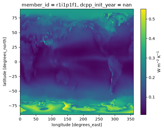
gm_swq_feedback = global_average(swq_feedback.mean(dim='month')).load()
gm_swq_feedbackCould not determine bucket type for bucket name cmip6: Your default credentials were not found. To set up Application Default Credentials, see https://cloud.google.com/docs/authentication/external/set-up-adc for more information., falling back to GCSFileSystem
Could not determine bucket type for bucket name cmip6: Your default credentials were not found. To set up Application Default Credentials, see https://cloud.google.com/docs/authentication/external/set-up-adc for more information., falling back to GCSFileSystem
Could not determine bucket type for bucket name cmip6: Your default credentials were not found. To set up Application Default Credentials, see https://cloud.google.com/docs/authentication/external/set-up-adc for more information., falling back to GCSFileSystem
Could not determine bucket type for bucket name cmip6: Your default credentials were not found. To set up Application Default Credentials, see https://cloud.google.com/docs/authentication/external/set-up-adc for more information., falling back to GCSFileSystem
Could not determine bucket type for bucket name cmip6: Your default credentials were not found. To set up Application Default Credentials, see https://cloud.google.com/docs/authentication/external/set-up-adc for more information., falling back to GCSFileSystem
Could not determine bucket type for bucket name cmip6: Your default credentials were not found. To set up Application Default Credentials, see https://cloud.google.com/docs/authentication/external/set-up-adc for more information., falling back to GCSFileSystem
Could not determine bucket type for bucket name cmip6: Your default credentials were not found. To set up Application Default Credentials, see https://cloud.google.com/docs/authentication/external/set-up-adc for more information., falling back to GCSFileSystem
Could not determine bucket type for bucket name cmip6: Your default credentials were not found. To set up Application Default Credentials, see https://cloud.google.com/docs/authentication/external/set-up-adc for more information., falling back to GCSFileSystem
Could not determine bucket type for bucket name cmip6: Your default credentials were not found. To set up Application Default Credentials, see https://cloud.google.com/docs/authentication/external/set-up-adc for more information., falling back to GCSFileSystem
Could not determine bucket type for bucket name cmip6: Your default credentials were not found. To set up Application Default Credentials, see https://cloud.google.com/docs/authentication/external/set-up-adc for more information., falling back to GCSFileSystem
Could not determine bucket type for bucket name cmip6: Your default credentials were not found. To set up Application Default Credentials, see https://cloud.google.com/docs/authentication/external/set-up-adc for more information., falling back to GCSFileSystem
Could not determine bucket type for bucket name cmip6: Your default credentials were not found. To set up Application Default Credentials, see https://cloud.google.com/docs/authentication/external/set-up-adc for more information., falling back to GCSFileSystem
Could not determine bucket type for bucket name cmip6: Your default credentials were not found. To set up Application Default Credentials, see https://cloud.google.com/docs/authentication/external/set-up-adc for more information., falling back to GCSFileSystem
Could not determine bucket type for bucket name cmip6: Your default credentials were not found. To set up Application Default Credentials, see https://cloud.google.com/docs/authentication/external/set-up-adc for more information., falling back to GCSFileSystem
Could not determine bucket type for bucket name cmip6: Your default credentials were not found. To set up Application Default Credentials, see https://cloud.google.com/docs/authentication/external/set-up-adc for more information., falling back to GCSFileSystem
Could not determine bucket type for bucket name cmip6: Your default credentials were not found. To set up Application Default Credentials, see https://cloud.google.com/docs/authentication/external/set-up-adc for more information., falling back to GCSFileSystem
Could not determine bucket type for bucket name cmip6: Your default credentials were not found. To set up Application Default Credentials, see https://cloud.google.com/docs/authentication/external/set-up-adc for more information., falling back to GCSFileSystem
Could not determine bucket type for bucket name cmip6: Your default credentials were not found. To set up Application Default Credentials, see https://cloud.google.com/docs/authentication/external/set-up-adc for more information., falling back to GCSFileSystem
Could not determine bucket type for bucket name cmip6: Your default credentials were not found. To set up Application Default Credentials, see https://cloud.google.com/docs/authentication/external/set-up-adc for more information., falling back to GCSFileSystem
Could not determine bucket type for bucket name cmip6: Your default credentials were not found. To set up Application Default Credentials, see https://cloud.google.com/docs/authentication/external/set-up-adc for more information., falling back to GCSFileSystem
Could not determine bucket type for bucket name cmip6: Your default credentials were not found. To set up Application Default Credentials, see https://cloud.google.com/docs/authentication/external/set-up-adc for more information., falling back to GCSFileSystem
Could not determine bucket type for bucket name cmip6: Your default credentials were not found. To set up Application Default Credentials, see https://cloud.google.com/docs/authentication/external/set-up-adc for more information., falling back to GCSFileSystem
Could not determine bucket type for bucket name cmip6: Your default credentials were not found. To set up Application Default Credentials, see https://cloud.google.com/docs/authentication/external/set-up-adc for more information., falling back to GCSFileSystem
Could not determine bucket type for bucket name cmip6: Your default credentials were not found. To set up Application Default Credentials, see https://cloud.google.com/docs/authentication/external/set-up-adc for more information., falling back to GCSFileSystem
Could not determine bucket type for bucket name cmip6: Your default credentials were not found. To set up Application Default Credentials, see https://cloud.google.com/docs/authentication/external/set-up-adc for more information., falling back to GCSFileSystem
Could not determine bucket type for bucket name cmip6: Your default credentials were not found. To set up Application Default Credentials, see https://cloud.google.com/docs/authentication/external/set-up-adc for more information., falling back to GCSFileSystem
Could not determine bucket type for bucket name cmip6: Your default credentials were not found. To set up Application Default Credentials, see https://cloud.google.com/docs/authentication/external/set-up-adc for more information., falling back to GCSFileSystem
Could not determine bucket type for bucket name cmip6: Your default credentials were not found. To set up Application Default Credentials, see https://cloud.google.com/docs/authentication/external/set-up-adc for more information., falling back to GCSFileSystem
Could not determine bucket type for bucket name cmip6: Your default credentials were not found. To set up Application Default Credentials, see https://cloud.google.com/docs/authentication/external/set-up-adc for more information., falling back to GCSFileSystem
Could not determine bucket type for bucket name cmip6: Your default credentials were not found. To set up Application Default Credentials, see https://cloud.google.com/docs/authentication/external/set-up-adc for more information., falling back to GCSFileSystem
Could not determine bucket type for bucket name cmip6: Your default credentials were not found. To set up Application Default Credentials, see https://cloud.google.com/docs/authentication/external/set-up-adc for more information., falling back to GCSFileSystem
Could not determine bucket type for bucket name cmip6: Your default credentials were not found. To set up Application Default Credentials, see https://cloud.google.com/docs/authentication/external/set-up-adc for more information., falling back to GCSFileSystem
Could not determine bucket type for bucket name cmip6: Your default credentials were not found. To set up Application Default Credentials, see https://cloud.google.com/docs/authentication/external/set-up-adc for more information., falling back to GCSFileSystem
Could not determine bucket type for bucket name cmip6: Your default credentials were not found. To set up Application Default Credentials, see https://cloud.google.com/docs/authentication/external/set-up-adc for more information., falling back to GCSFileSystem
Could not determine bucket type for bucket name cmip6: Your default credentials were not found. To set up Application Default Credentials, see https://cloud.google.com/docs/authentication/external/set-up-adc for more information., falling back to GCSFileSystem
Could not determine bucket type for bucket name cmip6: Your default credentials were not found. To set up Application Default Credentials, see https://cloud.google.com/docs/authentication/external/set-up-adc for more information., falling back to GCSFileSystem
Could not determine bucket type for bucket name cmip6: Your default credentials were not found. To set up Application Default Credentials, see https://cloud.google.com/docs/authentication/external/set-up-adc for more information., falling back to GCSFileSystem
Could not determine bucket type for bucket name cmip6: Your default credentials were not found. To set up Application Default Credentials, see https://cloud.google.com/docs/authentication/external/set-up-adc for more information., falling back to GCSFileSystem
Could not determine bucket type for bucket name cmip6: Your default credentials were not found. To set up Application Default Credentials, see https://cloud.google.com/docs/authentication/external/set-up-adc for more information., falling back to GCSFileSystem
Could not determine bucket type for bucket name cmip6: Your default credentials were not found. To set up Application Default Credentials, see https://cloud.google.com/docs/authentication/external/set-up-adc for more information., falling back to GCSFileSystem
Could not determine bucket type for bucket name cmip6: Your default credentials were not found. To set up Application Default Credentials, see https://cloud.google.com/docs/authentication/external/set-up-adc for more information., falling back to GCSFileSystem
Could not determine bucket type for bucket name cmip6: Your default credentials were not found. To set up Application Default Credentials, see https://cloud.google.com/docs/authentication/external/set-up-adc for more information., falling back to GCSFileSystem
Could not determine bucket type for bucket name cmip6: Your default credentials were not found. To set up Application Default Credentials, see https://cloud.google.com/docs/authentication/external/set-up-adc for more information., falling back to GCSFileSystem
Could not determine bucket type for bucket name cmip6: Your default credentials were not found. To set up Application Default Credentials, see https://cloud.google.com/docs/authentication/external/set-up-adc for more information., falling back to GCSFileSystem
Could not determine bucket type for bucket name cmip6: Your default credentials were not found. To set up Application Default Credentials, see https://cloud.google.com/docs/authentication/external/set-up-adc for more information., falling back to GCSFileSystem
Could not determine bucket type for bucket name cmip6: Your default credentials were not found. To set up Application Default Credentials, see https://cloud.google.com/docs/authentication/external/set-up-adc for more information., falling back to GCSFileSystem
Could not determine bucket type for bucket name cmip6: Your default credentials were not found. To set up Application Default Credentials, see https://cloud.google.com/docs/authentication/external/set-up-adc for more information., falling back to GCSFileSystem
Could not determine bucket type for bucket name cmip6: Your default credentials were not found. To set up Application Default Credentials, see https://cloud.google.com/docs/authentication/external/set-up-adc for more information., falling back to GCSFileSystem
Could not determine bucket type for bucket name cmip6: Your default credentials were not found. To set up Application Default Credentials, see https://cloud.google.com/docs/authentication/external/set-up-adc for more information., falling back to GCSFileSystem
Could not determine bucket type for bucket name cmip6: Your default credentials were not found. To set up Application Default Credentials, see https://cloud.google.com/docs/authentication/external/set-up-adc for more information., falling back to GCSFileSystem
Could not determine bucket type for bucket name cmip6: Your default credentials were not found. To set up Application Default Credentials, see https://cloud.google.com/docs/authentication/external/set-up-adc for more information., falling back to GCSFileSystem
Could not determine bucket type for bucket name cmip6: Your default credentials were not found. To set up Application Default Credentials, see https://cloud.google.com/docs/authentication/external/set-up-adc for more information., falling back to GCSFileSystem
Could not determine bucket type for bucket name cmip6: Your default credentials were not found. To set up Application Default Credentials, see https://cloud.google.com/docs/authentication/external/set-up-adc for more information., falling back to GCSFileSystem
Could not determine bucket type for bucket name cmip6: Your default credentials were not found. To set up Application Default Credentials, see https://cloud.google.com/docs/authentication/external/set-up-adc for more information., falling back to GCSFileSystem
Could not determine bucket type for bucket name cmip6: Your default credentials were not found. To set up Application Default Credentials, see https://cloud.google.com/docs/authentication/external/set-up-adc for more information., falling back to GCSFileSystem
Could not determine bucket type for bucket name cmip6: Your default credentials were not found. To set up Application Default Credentials, see https://cloud.google.com/docs/authentication/external/set-up-adc for more information., falling back to GCSFileSystem
Could not determine bucket type for bucket name cmip6: Your default credentials were not found. To set up Application Default Credentials, see https://cloud.google.com/docs/authentication/external/set-up-adc for more information., falling back to GCSFileSystem
Could not determine bucket type for bucket name cmip6: Your default credentials were not found. To set up Application Default Credentials, see https://cloud.google.com/docs/authentication/external/set-up-adc for more information., falling back to GCSFileSystem
Could not determine bucket type for bucket name cmip6: Your default credentials were not found. To set up Application Default Credentials, see https://cloud.google.com/docs/authentication/external/set-up-adc for more information., falling back to GCSFileSystem
Could not determine bucket type for bucket name cmip6: Your default credentials were not found. To set up Application Default Credentials, see https://cloud.google.com/docs/authentication/external/set-up-adc for more information., falling back to GCSFileSystem
Could not determine bucket type for bucket name cmip6: Your default credentials were not found. To set up Application Default Credentials, see https://cloud.google.com/docs/authentication/external/set-up-adc for more information., falling back to GCSFileSystem
Could not determine bucket type for bucket name cmip6: Your default credentials were not found. To set up Application Default Credentials, see https://cloud.google.com/docs/authentication/external/set-up-adc for more information., falling back to GCSFileSystem
Could not determine bucket type for bucket name cmip6: Your default credentials were not found. To set up Application Default Credentials, see https://cloud.google.com/docs/authentication/external/set-up-adc for more information., falling back to GCSFileSystem
Could not determine bucket type for bucket name cmip6: Your default credentials were not found. To set up Application Default Credentials, see https://cloud.google.com/docs/authentication/external/set-up-adc for more information., falling back to GCSFileSystem
Could not determine bucket type for bucket name cmip6: Your default credentials were not found. To set up Application Default Credentials, see https://cloud.google.com/docs/authentication/external/set-up-adc for more information., falling back to GCSFileSystem
Could not determine bucket type for bucket name cmip6: Your default credentials were not found. To set up Application Default Credentials, see https://cloud.google.com/docs/authentication/external/set-up-adc for more information., falling back to GCSFileSystem
Could not determine bucket type for bucket name cmip6: Your default credentials were not found. To set up Application Default Credentials, see https://cloud.google.com/docs/authentication/external/set-up-adc for more information., falling back to GCSFileSystem
Could not determine bucket type for bucket name cmip6: Your default credentials were not found. To set up Application Default Credentials, see https://cloud.google.com/docs/authentication/external/set-up-adc for more information., falling back to GCSFileSystem
Could not determine bucket type for bucket name cmip6: Your default credentials were not found. To set up Application Default Credentials, see https://cloud.google.com/docs/authentication/external/set-up-adc for more information., falling back to GCSFileSystem
Could not determine bucket type for bucket name cmip6: Your default credentials were not found. To set up Application Default Credentials, see https://cloud.google.com/docs/authentication/external/set-up-adc for more information., falling back to GCSFileSystem
Could not determine bucket type for bucket name cmip6: Your default credentials were not found. To set up Application Default Credentials, see https://cloud.google.com/docs/authentication/external/set-up-adc for more information., falling back to GCSFileSystem
Could not determine bucket type for bucket name cmip6: Your default credentials were not found. To set up Application Default Credentials, see https://cloud.google.com/docs/authentication/external/set-up-adc for more information., falling back to GCSFileSystem
Could not determine bucket type for bucket name cmip6: Your default credentials were not found. To set up Application Default Credentials, see https://cloud.google.com/docs/authentication/external/set-up-adc for more information., falling back to GCSFileSystem
Could not determine bucket type for bucket name cmip6: Your default credentials were not found. To set up Application Default Credentials, see https://cloud.google.com/docs/authentication/external/set-up-adc for more information., falling back to GCSFileSystem
Could not determine bucket type for bucket name cmip6: Your default credentials were not found. To set up Application Default Credentials, see https://cloud.google.com/docs/authentication/external/set-up-adc for more information., falling back to GCSFileSystem
Could not determine bucket type for bucket name cmip6: Your default credentials were not found. To set up Application Default Credentials, see https://cloud.google.com/docs/authentication/external/set-up-adc for more information., falling back to GCSFileSystem
Could not determine bucket type for bucket name cmip6: Your default credentials were not found. To set up Application Default Credentials, see https://cloud.google.com/docs/authentication/external/set-up-adc for more information., falling back to GCSFileSystem
Could not determine bucket type for bucket name cmip6: Your default credentials were not found. To set up Application Default Credentials, see https://cloud.google.com/docs/authentication/external/set-up-adc for more information., falling back to GCSFileSystem
Could not determine bucket type for bucket name cmip6: Your default credentials were not found. To set up Application Default Credentials, see https://cloud.google.com/docs/authentication/external/set-up-adc for more information., falling back to GCSFileSystem
Could not determine bucket type for bucket name cmip6: Your default credentials were not found. To set up Application Default Credentials, see https://cloud.google.com/docs/authentication/external/set-up-adc for more information., falling back to GCSFileSystem
Could not determine bucket type for bucket name cmip6: Your default credentials were not found. To set up Application Default Credentials, see https://cloud.google.com/docs/authentication/external/set-up-adc for more information., falling back to GCSFileSystem
Could not determine bucket type for bucket name cmip6: Your default credentials were not found. To set up Application Default Credentials, see https://cloud.google.com/docs/authentication/external/set-up-adc for more information., falling back to GCSFileSystem
Could not determine bucket type for bucket name cmip6: Your default credentials were not found. To set up Application Default Credentials, see https://cloud.google.com/docs/authentication/external/set-up-adc for more information., falling back to GCSFileSystem
Could not determine bucket type for bucket name cmip6: Your default credentials were not found. To set up Application Default Credentials, see https://cloud.google.com/docs/authentication/external/set-up-adc for more information., falling back to GCSFileSystem
Could not determine bucket type for bucket name cmip6: Your default credentials were not found. To set up Application Default Credentials, see https://cloud.google.com/docs/authentication/external/set-up-adc for more information., falling back to GCSFileSystem
Could not determine bucket type for bucket name cmip6: Your default credentials were not found. To set up Application Default Credentials, see https://cloud.google.com/docs/authentication/external/set-up-adc for more information., falling back to GCSFileSystem
Could not determine bucket type for bucket name cmip6: Your default credentials were not found. To set up Application Default Credentials, see https://cloud.google.com/docs/authentication/external/set-up-adc for more information., falling back to GCSFileSystem
Could not determine bucket type for bucket name cmip6: Your default credentials were not found. To set up Application Default Credentials, see https://cloud.google.com/docs/authentication/external/set-up-adc for more information., falling back to GCSFileSystem
Could not determine bucket type for bucket name cmip6: Your default credentials were not found. To set up Application Default Credentials, see https://cloud.google.com/docs/authentication/external/set-up-adc for more information., falling back to GCSFileSystem
Could not determine bucket type for bucket name cmip6: Your default credentials were not found. To set up Application Default Credentials, see https://cloud.google.com/docs/authentication/external/set-up-adc for more information., falling back to GCSFileSystem
Could not determine bucket type for bucket name cmip6: Your default credentials were not found. To set up Application Default Credentials, see https://cloud.google.com/docs/authentication/external/set-up-adc for more information., falling back to GCSFileSystem
Could not determine bucket type for bucket name cmip6: Your default credentials were not found. To set up Application Default Credentials, see https://cloud.google.com/docs/authentication/external/set-up-adc for more information., falling back to GCSFileSystem
Could not determine bucket type for bucket name cmip6: Your default credentials were not found. To set up Application Default Credentials, see https://cloud.google.com/docs/authentication/external/set-up-adc for more information., falling back to GCSFileSystem
Could not determine bucket type for bucket name cmip6: Your default credentials were not found. To set up Application Default Credentials, see https://cloud.google.com/docs/authentication/external/set-up-adc for more information., falling back to GCSFileSystem
Could not determine bucket type for bucket name cmip6: Your default credentials were not found. To set up Application Default Credentials, see https://cloud.google.com/docs/authentication/external/set-up-adc for more information., falling back to GCSFileSystem
Could not determine bucket type for bucket name cmip6: Your default credentials were not found. To set up Application Default Credentials, see https://cloud.google.com/docs/authentication/external/set-up-adc for more information., falling back to GCSFileSystem
Could not determine bucket type for bucket name cmip6: Your default credentials were not found. To set up Application Default Credentials, see https://cloud.google.com/docs/authentication/external/set-up-adc for more information., falling back to GCSFileSystem
Could not determine bucket type for bucket name cmip6: Your default credentials were not found. To set up Application Default Credentials, see https://cloud.google.com/docs/authentication/external/set-up-adc for more information., falling back to GCSFileSystem
Could not determine bucket type for bucket name cmip6: Your default credentials were not found. To set up Application Default Credentials, see https://cloud.google.com/docs/authentication/external/set-up-adc for more information., falling back to GCSFileSystem
Could not determine bucket type for bucket name cmip6: Your default credentials were not found. To set up Application Default Credentials, see https://cloud.google.com/docs/authentication/external/set-up-adc for more information., falling back to GCSFileSystem
Could not determine bucket type for bucket name cmip6: Your default credentials were not found. To set up Application Default Credentials, see https://cloud.google.com/docs/authentication/external/set-up-adc for more information., falling back to GCSFileSystem
Could not determine bucket type for bucket name cmip6: Your default credentials were not found. To set up Application Default Credentials, see https://cloud.google.com/docs/authentication/external/set-up-adc for more information., falling back to GCSFileSystem
Could not determine bucket type for bucket name cmip6: Your default credentials were not found. To set up Application Default Credentials, see https://cloud.google.com/docs/authentication/external/set-up-adc for more information., falling back to GCSFileSystem
Could not determine bucket type for bucket name cmip6: Your default credentials were not found. To set up Application Default Credentials, see https://cloud.google.com/docs/authentication/external/set-up-adc for more information., falling back to GCSFileSystem
Could not determine bucket type for bucket name cmip6: Your default credentials were not found. To set up Application Default Credentials, see https://cloud.google.com/docs/authentication/external/set-up-adc for more information., falling back to GCSFileSystem
Could not determine bucket type for bucket name cmip6: Your default credentials were not found. To set up Application Default Credentials, see https://cloud.google.com/docs/authentication/external/set-up-adc for more information., falling back to GCSFileSystem
Could not determine bucket type for bucket name cmip6: Your default credentials were not found. To set up Application Default Credentials, see https://cloud.google.com/docs/authentication/external/set-up-adc for more information., falling back to GCSFileSystem
Could not determine bucket type for bucket name cmip6: Your default credentials were not found. To set up Application Default Credentials, see https://cloud.google.com/docs/authentication/external/set-up-adc for more information., falling back to GCSFileSystem
Could not determine bucket type for bucket name cmip6: Your default credentials were not found. To set up Application Default Credentials, see https://cloud.google.com/docs/authentication/external/set-up-adc for more information., falling back to GCSFileSystem
Could not determine bucket type for bucket name cmip6: Your default credentials were not found. To set up Application Default Credentials, see https://cloud.google.com/docs/authentication/external/set-up-adc for more information., falling back to GCSFileSystem
Could not determine bucket type for bucket name cmip6: Your default credentials were not found. To set up Application Default Credentials, see https://cloud.google.com/docs/authentication/external/set-up-adc for more information., falling back to GCSFileSystem
Could not determine bucket type for bucket name cmip6: Your default credentials were not found. To set up Application Default Credentials, see https://cloud.google.com/docs/authentication/external/set-up-adc for more information., falling back to GCSFileSystem
Could not determine bucket type for bucket name cmip6: Your default credentials were not found. To set up Application Default Credentials, see https://cloud.google.com/docs/authentication/external/set-up-adc for more information., falling back to GCSFileSystem
Could not determine bucket type for bucket name cmip6: Your default credentials were not found. To set up Application Default Credentials, see https://cloud.google.com/docs/authentication/external/set-up-adc for more information., falling back to GCSFileSystem
Could not determine bucket type for bucket name cmip6: Your default credentials were not found. To set up Application Default Credentials, see https://cloud.google.com/docs/authentication/external/set-up-adc for more information., falling back to GCSFileSystem
Could not determine bucket type for bucket name cmip6: Your default credentials were not found. To set up Application Default Credentials, see https://cloud.google.com/docs/authentication/external/set-up-adc for more information., falling back to GCSFileSystem
Could not determine bucket type for bucket name cmip6: Your default credentials were not found. To set up Application Default Credentials, see https://cloud.google.com/docs/authentication/external/set-up-adc for more information., falling back to GCSFileSystem
Could not determine bucket type for bucket name cmip6: Your default credentials were not found. To set up Application Default Credentials, see https://cloud.google.com/docs/authentication/external/set-up-adc for more information., falling back to GCSFileSystem
Could not determine bucket type for bucket name cmip6: Your default credentials were not found. To set up Application Default Credentials, see https://cloud.google.com/docs/authentication/external/set-up-adc for more information., falling back to GCSFileSystem
Could not determine bucket type for bucket name cmip6: Your default credentials were not found. To set up Application Default Credentials, see https://cloud.google.com/docs/authentication/external/set-up-adc for more information., falling back to GCSFileSystem
Could not determine bucket type for bucket name cmip6: Your default credentials were not found. To set up Application Default Credentials, see https://cloud.google.com/docs/authentication/external/set-up-adc for more information., falling back to GCSFileSystem
Could not determine bucket type for bucket name cmip6: Your default credentials were not found. To set up Application Default Credentials, see https://cloud.google.com/docs/authentication/external/set-up-adc for more information., falling back to GCSFileSystem
Could not determine bucket type for bucket name cmip6: Your default credentials were not found. To set up Application Default Credentials, see https://cloud.google.com/docs/authentication/external/set-up-adc for more information., falling back to GCSFileSystem
Could not determine bucket type for bucket name cmip6: Your default credentials were not found. To set up Application Default Credentials, see https://cloud.google.com/docs/authentication/external/set-up-adc for more information., falling back to GCSFileSystem
Could not determine bucket type for bucket name cmip6: Your default credentials were not found. To set up Application Default Credentials, see https://cloud.google.com/docs/authentication/external/set-up-adc for more information., falling back to GCSFileSystem
Could not determine bucket type for bucket name cmip6: Your default credentials were not found. To set up Application Default Credentials, see https://cloud.google.com/docs/authentication/external/set-up-adc for more information., falling back to GCSFileSystem
Could not determine bucket type for bucket name cmip6: Your default credentials were not found. To set up Application Default Credentials, see https://cloud.google.com/docs/authentication/external/set-up-adc for more information., falling back to GCSFileSystem
Could not determine bucket type for bucket name cmip6: Your default credentials were not found. To set up Application Default Credentials, see https://cloud.google.com/docs/authentication/external/set-up-adc for more information., falling back to GCSFileSystem
Could not determine bucket type for bucket name cmip6: Your default credentials were not found. To set up Application Default Credentials, see https://cloud.google.com/docs/authentication/external/set-up-adc for more information., falling back to GCSFileSystem
Could not determine bucket type for bucket name cmip6: Your default credentials were not found. To set up Application Default Credentials, see https://cloud.google.com/docs/authentication/external/set-up-adc for more information., falling back to GCSFileSystem
Could not determine bucket type for bucket name cmip6: Your default credentials were not found. To set up Application Default Credentials, see https://cloud.google.com/docs/authentication/external/set-up-adc for more information., falling back to GCSFileSystem
Could not determine bucket type for bucket name cmip6: Your default credentials were not found. To set up Application Default Credentials, see https://cloud.google.com/docs/authentication/external/set-up-adc for more information., falling back to GCSFileSystem
Could not determine bucket type for bucket name cmip6: Your default credentials were not found. To set up Application Default Credentials, see https://cloud.google.com/docs/authentication/external/set-up-adc for more information., falling back to GCSFileSystem
Could not determine bucket type for bucket name cmip6: Your default credentials were not found. To set up Application Default Credentials, see https://cloud.google.com/docs/authentication/external/set-up-adc for more information., falling back to GCSFileSystem
Could not determine bucket type for bucket name cmip6: Your default credentials were not found. To set up Application Default Credentials, see https://cloud.google.com/docs/authentication/external/set-up-adc for more information., falling back to GCSFileSystem
Could not determine bucket type for bucket name cmip6: Your default credentials were not found. To set up Application Default Credentials, see https://cloud.google.com/docs/authentication/external/set-up-adc for more information., falling back to GCSFileSystem
Could not determine bucket type for bucket name cmip6: Your default credentials were not found. To set up Application Default Credentials, see https://cloud.google.com/docs/authentication/external/set-up-adc for more information., falling back to GCSFileSystem
Could not determine bucket type for bucket name cmip6: Your default credentials were not found. To set up Application Default Credentials, see https://cloud.google.com/docs/authentication/external/set-up-adc for more information., falling back to GCSFileSystem
Could not determine bucket type for bucket name cmip6: Your default credentials were not found. To set up Application Default Credentials, see https://cloud.google.com/docs/authentication/external/set-up-adc for more information., falling back to GCSFileSystem
Could not determine bucket type for bucket name cmip6: Your default credentials were not found. To set up Application Default Credentials, see https://cloud.google.com/docs/authentication/external/set-up-adc for more information., falling back to GCSFileSystem
Could not determine bucket type for bucket name cmip6: Your default credentials were not found. To set up Application Default Credentials, see https://cloud.google.com/docs/authentication/external/set-up-adc for more information., falling back to GCSFileSystem
Could not determine bucket type for bucket name cmip6: Your default credentials were not found. To set up Application Default Credentials, see https://cloud.google.com/docs/authentication/external/set-up-adc for more information., falling back to GCSFileSystem
Could not determine bucket type for bucket name cmip6: Your default credentials were not found. To set up Application Default Credentials, see https://cloud.google.com/docs/authentication/external/set-up-adc for more information., falling back to GCSFileSystem
Could not determine bucket type for bucket name cmip6: Your default credentials were not found. To set up Application Default Credentials, see https://cloud.google.com/docs/authentication/external/set-up-adc for more information., falling back to GCSFileSystem
Could not determine bucket type for bucket name cmip6: Your default credentials were not found. To set up Application Default Credentials, see https://cloud.google.com/docs/authentication/external/set-up-adc for more information., falling back to GCSFileSystem
Could not determine bucket type for bucket name cmip6: Your default credentials were not found. To set up Application Default Credentials, see https://cloud.google.com/docs/authentication/external/set-up-adc for more information., falling back to GCSFileSystem
Could not determine bucket type for bucket name cmip6: Your default credentials were not found. To set up Application Default Credentials, see https://cloud.google.com/docs/authentication/external/set-up-adc for more information., falling back to GCSFileSystem
Could not determine bucket type for bucket name cmip6: Your default credentials were not found. To set up Application Default Credentials, see https://cloud.google.com/docs/authentication/external/set-up-adc for more information., falling back to GCSFileSystem
Could not determine bucket type for bucket name cmip6: Your default credentials were not found. To set up Application Default Credentials, see https://cloud.google.com/docs/authentication/external/set-up-adc for more information., falling back to GCSFileSystem
Could not determine bucket type for bucket name cmip6: Your default credentials were not found. To set up Application Default Credentials, see https://cloud.google.com/docs/authentication/external/set-up-adc for more information., falling back to GCSFileSystem
Could not determine bucket type for bucket name cmip6: Your default credentials were not found. To set up Application Default Credentials, see https://cloud.google.com/docs/authentication/external/set-up-adc for more information., falling back to GCSFileSystem
Could not determine bucket type for bucket name cmip6: Your default credentials were not found. To set up Application Default Credentials, see https://cloud.google.com/docs/authentication/external/set-up-adc for more information., falling back to GCSFileSystem
Could not determine bucket type for bucket name cmip6: Your default credentials were not found. To set up Application Default Credentials, see https://cloud.google.com/docs/authentication/external/set-up-adc for more information., falling back to GCSFileSystem
Could not determine bucket type for bucket name cmip6: Your default credentials were not found. To set up Application Default Credentials, see https://cloud.google.com/docs/authentication/external/set-up-adc for more information., falling back to GCSFileSystem
Could not determine bucket type for bucket name cmip6: Your default credentials were not found. To set up Application Default Credentials, see https://cloud.google.com/docs/authentication/external/set-up-adc for more information., falling back to GCSFileSystem
Could not determine bucket type for bucket name cmip6: Your default credentials were not found. To set up Application Default Credentials, see https://cloud.google.com/docs/authentication/external/set-up-adc for more information., falling back to GCSFileSystem
Could not determine bucket type for bucket name cmip6: Your default credentials were not found. To set up Application Default Credentials, see https://cloud.google.com/docs/authentication/external/set-up-adc for more information., falling back to GCSFileSystem
Could not determine bucket type for bucket name cmip6: Your default credentials were not found. To set up Application Default Credentials, see https://cloud.google.com/docs/authentication/external/set-up-adc for more information., falling back to GCSFileSystem
Could not determine bucket type for bucket name cmip6: Your default credentials were not found. To set up Application Default Credentials, see https://cloud.google.com/docs/authentication/external/set-up-adc for more information., falling back to GCSFileSystem
Could not determine bucket type for bucket name cmip6: Your default credentials were not found. To set up Application Default Credentials, see https://cloud.google.com/docs/authentication/external/set-up-adc for more information., falling back to GCSFileSystem
Could not determine bucket type for bucket name cmip6: Your default credentials were not found. To set up Application Default Credentials, see https://cloud.google.com/docs/authentication/external/set-up-adc for more information., falling back to GCSFileSystem
Could not determine bucket type for bucket name cmip6: Your default credentials were not found. To set up Application Default Credentials, see https://cloud.google.com/docs/authentication/external/set-up-adc for more information., falling back to GCSFileSystem
Could not determine bucket type for bucket name cmip6: Your default credentials were not found. To set up Application Default Credentials, see https://cloud.google.com/docs/authentication/external/set-up-adc for more information., falling back to GCSFileSystem
Could not determine bucket type for bucket name cmip6: Your default credentials were not found. To set up Application Default Credentials, see https://cloud.google.com/docs/authentication/external/set-up-adc for more information., falling back to GCSFileSystem
Could not determine bucket type for bucket name cmip6: Your default credentials were not found. To set up Application Default Credentials, see https://cloud.google.com/docs/authentication/external/set-up-adc for more information., falling back to GCSFileSystem
Could not determine bucket type for bucket name cmip6: Your default credentials were not found. To set up Application Default Credentials, see https://cloud.google.com/docs/authentication/external/set-up-adc for more information., falling back to GCSFileSystem
Could not determine bucket type for bucket name cmip6: Your default credentials were not found. To set up Application Default Credentials, see https://cloud.google.com/docs/authentication/external/set-up-adc for more information., falling back to GCSFileSystem
Could not determine bucket type for bucket name cmip6: Your default credentials were not found. To set up Application Default Credentials, see https://cloud.google.com/docs/authentication/external/set-up-adc for more information., falling back to GCSFileSystem
Could not determine bucket type for bucket name cmip6: Your default credentials were not found. To set up Application Default Credentials, see https://cloud.google.com/docs/authentication/external/set-up-adc for more information., falling back to GCSFileSystem
Could not determine bucket type for bucket name cmip6: Your default credentials were not found. To set up Application Default Credentials, see https://cloud.google.com/docs/authentication/external/set-up-adc for more information., falling back to GCSFileSystem
Could not determine bucket type for bucket name cmip6: Your default credentials were not found. To set up Application Default Credentials, see https://cloud.google.com/docs/authentication/external/set-up-adc for more information., falling back to GCSFileSystem
Could not determine bucket type for bucket name cmip6: Your default credentials were not found. To set up Application Default Credentials, see https://cloud.google.com/docs/authentication/external/set-up-adc for more information., falling back to GCSFileSystem
Could not determine bucket type for bucket name cmip6: Your default credentials were not found. To set up Application Default Credentials, see https://cloud.google.com/docs/authentication/external/set-up-adc for more information., falling back to GCSFileSystem
Could not determine bucket type for bucket name cmip6: Your default credentials were not found. To set up Application Default Credentials, see https://cloud.google.com/docs/authentication/external/set-up-adc for more information., falling back to GCSFileSystem
Could not determine bucket type for bucket name cmip6: Your default credentials were not found. To set up Application Default Credentials, see https://cloud.google.com/docs/authentication/external/set-up-adc for more information., falling back to GCSFileSystem
Could not determine bucket type for bucket name cmip6: Your default credentials were not found. To set up Application Default Credentials, see https://cloud.google.com/docs/authentication/external/set-up-adc for more information., falling back to GCSFileSystem
Could not determine bucket type for bucket name cmip6: Your default credentials were not found. To set up Application Default Credentials, see https://cloud.google.com/docs/authentication/external/set-up-adc for more information., falling back to GCSFileSystem
Could not determine bucket type for bucket name cmip6: Your default credentials were not found. To set up Application Default Credentials, see https://cloud.google.com/docs/authentication/external/set-up-adc for more information., falling back to GCSFileSystem
Could not determine bucket type for bucket name cmip6: Your default credentials were not found. To set up Application Default Credentials, see https://cloud.google.com/docs/authentication/external/set-up-adc for more information., falling back to GCSFileSystem
Could not determine bucket type for bucket name cmip6: Your default credentials were not found. To set up Application Default Credentials, see https://cloud.google.com/docs/authentication/external/set-up-adc for more information., falling back to GCSFileSystem
Could not determine bucket type for bucket name cmip6: Your default credentials were not found. To set up Application Default Credentials, see https://cloud.google.com/docs/authentication/external/set-up-adc for more information., falling back to GCSFileSystem
Could not determine bucket type for bucket name cmip6: Your default credentials were not found. To set up Application Default Credentials, see https://cloud.google.com/docs/authentication/external/set-up-adc for more information., falling back to GCSFileSystem
Could not determine bucket type for bucket name cmip6: Your default credentials were not found. To set up Application Default Credentials, see https://cloud.google.com/docs/authentication/external/set-up-adc for more information., falling back to GCSFileSystem
Could not determine bucket type for bucket name cmip6: Your default credentials were not found. To set up Application Default Credentials, see https://cloud.google.com/docs/authentication/external/set-up-adc for more information., falling back to GCSFileSystem
Could not determine bucket type for bucket name cmip6: Your default credentials were not found. To set up Application Default Credentials, see https://cloud.google.com/docs/authentication/external/set-up-adc for more information., falling back to GCSFileSystem
Could not determine bucket type for bucket name cmip6: Your default credentials were not found. To set up Application Default Credentials, see https://cloud.google.com/docs/authentication/external/set-up-adc for more information., falling back to GCSFileSystem
Could not determine bucket type for bucket name cmip6: Your default credentials were not found. To set up Application Default Credentials, see https://cloud.google.com/docs/authentication/external/set-up-adc for more information., falling back to GCSFileSystem
Could not determine bucket type for bucket name cmip6: Your default credentials were not found. To set up Application Default Credentials, see https://cloud.google.com/docs/authentication/external/set-up-adc for more information., falling back to GCSFileSystem
Could not determine bucket type for bucket name cmip6: Your default credentials were not found. To set up Application Default Credentials, see https://cloud.google.com/docs/authentication/external/set-up-adc for more information., falling back to GCSFileSystem
Could not determine bucket type for bucket name cmip6: Your default credentials were not found. To set up Application Default Credentials, see https://cloud.google.com/docs/authentication/external/set-up-adc for more information., falling back to GCSFileSystem
Could not determine bucket type for bucket name cmip6: Your default credentials were not found. To set up Application Default Credentials, see https://cloud.google.com/docs/authentication/external/set-up-adc for more information., falling back to GCSFileSystem
Could not determine bucket type for bucket name cmip6: Your default credentials were not found. To set up Application Default Credentials, see https://cloud.google.com/docs/authentication/external/set-up-adc for more information., falling back to GCSFileSystem
Could not determine bucket type for bucket name cmip6: Your default credentials were not found. To set up Application Default Credentials, see https://cloud.google.com/docs/authentication/external/set-up-adc for more information., falling back to GCSFileSystem
Could not determine bucket type for bucket name cmip6: Your default credentials were not found. To set up Application Default Credentials, see https://cloud.google.com/docs/authentication/external/set-up-adc for more information., falling back to GCSFileSystem
Could not determine bucket type for bucket name cmip6: Your default credentials were not found. To set up Application Default Credentials, see https://cloud.google.com/docs/authentication/external/set-up-adc for more information., falling back to GCSFileSystem
Could not determine bucket type for bucket name cmip6: Your default credentials were not found. To set up Application Default Credentials, see https://cloud.google.com/docs/authentication/external/set-up-adc for more information., falling back to GCSFileSystem
Could not determine bucket type for bucket name cmip6: Your default credentials were not found. To set up Application Default Credentials, see https://cloud.google.com/docs/authentication/external/set-up-adc for more information., falling back to GCSFileSystem
Could not determine bucket type for bucket name cmip6: Your default credentials were not found. To set up Application Default Credentials, see https://cloud.google.com/docs/authentication/external/set-up-adc for more information., falling back to GCSFileSystem
Could not determine bucket type for bucket name cmip6: Your default credentials were not found. To set up Application Default Credentials, see https://cloud.google.com/docs/authentication/external/set-up-adc for more information., falling back to GCSFileSystem
Could not determine bucket type for bucket name cmip6: Your default credentials were not found. To set up Application Default Credentials, see https://cloud.google.com/docs/authentication/external/set-up-adc for more information., falling back to GCSFileSystem
Could not determine bucket type for bucket name cmip6: Your default credentials were not found. To set up Application Default Credentials, see https://cloud.google.com/docs/authentication/external/set-up-adc for more information., falling back to GCSFileSystem
Could not determine bucket type for bucket name cmip6: Your default credentials were not found. To set up Application Default Credentials, see https://cloud.google.com/docs/authentication/external/set-up-adc for more information., falling back to GCSFileSystem
Could not determine bucket type for bucket name cmip6: Your default credentials were not found. To set up Application Default Credentials, see https://cloud.google.com/docs/authentication/external/set-up-adc for more information., falling back to GCSFileSystem
Could not determine bucket type for bucket name cmip6: Your default credentials were not found. To set up Application Default Credentials, see https://cloud.google.com/docs/authentication/external/set-up-adc for more information., falling back to GCSFileSystem
Could not determine bucket type for bucket name cmip6: Your default credentials were not found. To set up Application Default Credentials, see https://cloud.google.com/docs/authentication/external/set-up-adc for more information., falling back to GCSFileSystem
Could not determine bucket type for bucket name cmip6: Your default credentials were not found. To set up Application Default Credentials, see https://cloud.google.com/docs/authentication/external/set-up-adc for more information., falling back to GCSFileSystem
Could not determine bucket type for bucket name cmip6: Your default credentials were not found. To set up Application Default Credentials, see https://cloud.google.com/docs/authentication/external/set-up-adc for more information., falling back to GCSFileSystem
Could not determine bucket type for bucket name cmip6: Your default credentials were not found. To set up Application Default Credentials, see https://cloud.google.com/docs/authentication/external/set-up-adc for more information., falling back to GCSFileSystem
Could not determine bucket type for bucket name cmip6: Your default credentials were not found. To set up Application Default Credentials, see https://cloud.google.com/docs/authentication/external/set-up-adc for more information., falling back to GCSFileSystem
Could not determine bucket type for bucket name cmip6: Your default credentials were not found. To set up Application Default Credentials, see https://cloud.google.com/docs/authentication/external/set-up-adc for more information., falling back to GCSFileSystem
Could not determine bucket type for bucket name cmip6: Your default credentials were not found. To set up Application Default Credentials, see https://cloud.google.com/docs/authentication/external/set-up-adc for more information., falling back to GCSFileSystem
Could not determine bucket type for bucket name cmip6: Your default credentials were not found. To set up Application Default Credentials, see https://cloud.google.com/docs/authentication/external/set-up-adc for more information., falling back to GCSFileSystem
Could not determine bucket type for bucket name cmip6: Your default credentials were not found. To set up Application Default Credentials, see https://cloud.google.com/docs/authentication/external/set-up-adc for more information., falling back to GCSFileSystem
Could not determine bucket type for bucket name cmip6: Your default credentials were not found. To set up Application Default Credentials, see https://cloud.google.com/docs/authentication/external/set-up-adc for more information., falling back to GCSFileSystem
Could not determine bucket type for bucket name cmip6: Your default credentials were not found. To set up Application Default Credentials, see https://cloud.google.com/docs/authentication/external/set-up-adc for more information., falling back to GCSFileSystem
Could not determine bucket type for bucket name cmip6: Your default credentials were not found. To set up Application Default Credentials, see https://cloud.google.com/docs/authentication/external/set-up-adc for more information., falling back to GCSFileSystem
Could not determine bucket type for bucket name cmip6: Your default credentials were not found. To set up Application Default Credentials, see https://cloud.google.com/docs/authentication/external/set-up-adc for more information., falling back to GCSFileSystem
Could not determine bucket type for bucket name cmip6: Your default credentials were not found. To set up Application Default Credentials, see https://cloud.google.com/docs/authentication/external/set-up-adc for more information., falling back to GCSFileSystem
Could not determine bucket type for bucket name cmip6: Your default credentials were not found. To set up Application Default Credentials, see https://cloud.google.com/docs/authentication/external/set-up-adc for more information., falling back to GCSFileSystem
Could not determine bucket type for bucket name cmip6: Your default credentials were not found. To set up Application Default Credentials, see https://cloud.google.com/docs/authentication/external/set-up-adc for more information., falling back to GCSFileSystem
Could not determine bucket type for bucket name cmip6: Your default credentials were not found. To set up Application Default Credentials, see https://cloud.google.com/docs/authentication/external/set-up-adc for more information., falling back to GCSFileSystem
Could not determine bucket type for bucket name cmip6: Your default credentials were not found. To set up Application Default Credentials, see https://cloud.google.com/docs/authentication/external/set-up-adc for more information., falling back to GCSFileSystem
Could not determine bucket type for bucket name cmip6: Your default credentials were not found. To set up Application Default Credentials, see https://cloud.google.com/docs/authentication/external/set-up-adc for more information., falling back to GCSFileSystem
Could not determine bucket type for bucket name cmip6: Your default credentials were not found. To set up Application Default Credentials, see https://cloud.google.com/docs/authentication/external/set-up-adc for more information., falling back to GCSFileSystem
Could not determine bucket type for bucket name cmip6: Your default credentials were not found. To set up Application Default Credentials, see https://cloud.google.com/docs/authentication/external/set-up-adc for more information., falling back to GCSFileSystem
Could not determine bucket type for bucket name cmip6: Your default credentials were not found. To set up Application Default Credentials, see https://cloud.google.com/docs/authentication/external/set-up-adc for more information., falling back to GCSFileSystem
Could not determine bucket type for bucket name cmip6: Your default credentials were not found. To set up Application Default Credentials, see https://cloud.google.com/docs/authentication/external/set-up-adc for more information., falling back to GCSFileSystem
Could not determine bucket type for bucket name cmip6: Your default credentials were not found. To set up Application Default Credentials, see https://cloud.google.com/docs/authentication/external/set-up-adc for more information., falling back to GCSFileSystem
Could not determine bucket type for bucket name cmip6: Your default credentials were not found. To set up Application Default Credentials, see https://cloud.google.com/docs/authentication/external/set-up-adc for more information., falling back to GCSFileSystem
Could not determine bucket type for bucket name cmip6: Your default credentials were not found. To set up Application Default Credentials, see https://cloud.google.com/docs/authentication/external/set-up-adc for more information., falling back to GCSFileSystem
Could not determine bucket type for bucket name cmip6: Your default credentials were not found. To set up Application Default Credentials, see https://cloud.google.com/docs/authentication/external/set-up-adc for more information., falling back to GCSFileSystem
Could not determine bucket type for bucket name cmip6: Your default credentials were not found. To set up Application Default Credentials, see https://cloud.google.com/docs/authentication/external/set-up-adc for more information., falling back to GCSFileSystem
Could not determine bucket type for bucket name cmip6: Your default credentials were not found. To set up Application Default Credentials, see https://cloud.google.com/docs/authentication/external/set-up-adc for more information., falling back to GCSFileSystem
Could not determine bucket type for bucket name cmip6: Your default credentials were not found. To set up Application Default Credentials, see https://cloud.google.com/docs/authentication/external/set-up-adc for more information., falling back to GCSFileSystem
Could not determine bucket type for bucket name cmip6: Your default credentials were not found. To set up Application Default Credentials, see https://cloud.google.com/docs/authentication/external/set-up-adc for more information., falling back to GCSFileSystem
Could not determine bucket type for bucket name cmip6: Your default credentials were not found. To set up Application Default Credentials, see https://cloud.google.com/docs/authentication/external/set-up-adc for more information., falling back to GCSFileSystem
Could not determine bucket type for bucket name cmip6: Your default credentials were not found. To set up Application Default Credentials, see https://cloud.google.com/docs/authentication/external/set-up-adc for more information., falling back to GCSFileSystem
Could not determine bucket type for bucket name cmip6: Your default credentials were not found. To set up Application Default Credentials, see https://cloud.google.com/docs/authentication/external/set-up-adc for more information., falling back to GCSFileSystem
Could not determine bucket type for bucket name cmip6: Your default credentials were not found. To set up Application Default Credentials, see https://cloud.google.com/docs/authentication/external/set-up-adc for more information., falling back to GCSFileSystem
Could not determine bucket type for bucket name cmip6: Your default credentials were not found. To set up Application Default Credentials, see https://cloud.google.com/docs/authentication/external/set-up-adc for more information., falling back to GCSFileSystem
Could not determine bucket type for bucket name cmip6: Your default credentials were not found. To set up Application Default Credentials, see https://cloud.google.com/docs/authentication/external/set-up-adc for more information., falling back to GCSFileSystem
Could not determine bucket type for bucket name cmip6: Your default credentials were not found. To set up Application Default Credentials, see https://cloud.google.com/docs/authentication/external/set-up-adc for more information., falling back to GCSFileSystem
Could not determine bucket type for bucket name cmip6: Your default credentials were not found. To set up Application Default Credentials, see https://cloud.google.com/docs/authentication/external/set-up-adc for more information., falling back to GCSFileSystem
Could not determine bucket type for bucket name cmip6: Your default credentials were not found. To set up Application Default Credentials, see https://cloud.google.com/docs/authentication/external/set-up-adc for more information., falling back to GCSFileSystem
Could not determine bucket type for bucket name cmip6: Your default credentials were not found. To set up Application Default Credentials, see https://cloud.google.com/docs/authentication/external/set-up-adc for more information., falling back to GCSFileSystem
Could not determine bucket type for bucket name cmip6: Your default credentials were not found. To set up Application Default Credentials, see https://cloud.google.com/docs/authentication/external/set-up-adc for more information., falling back to GCSFileSystem
Could not determine bucket type for bucket name cmip6: Your default credentials were not found. To set up Application Default Credentials, see https://cloud.google.com/docs/authentication/external/set-up-adc for more information., falling back to GCSFileSystem
Could not determine bucket type for bucket name cmip6: Your default credentials were not found. To set up Application Default Credentials, see https://cloud.google.com/docs/authentication/external/set-up-adc for more information., falling back to GCSFileSystem
Could not determine bucket type for bucket name cmip6: Your default credentials were not found. To set up Application Default Credentials, see https://cloud.google.com/docs/authentication/external/set-up-adc for more information., falling back to GCSFileSystem
Could not determine bucket type for bucket name cmip6: Your default credentials were not found. To set up Application Default Credentials, see https://cloud.google.com/docs/authentication/external/set-up-adc for more information., falling back to GCSFileSystem
Could not determine bucket type for bucket name cmip6: Your default credentials were not found. To set up Application Default Credentials, see https://cloud.google.com/docs/authentication/external/set-up-adc for more information., falling back to GCSFileSystem
Could not determine bucket type for bucket name cmip6: Your default credentials were not found. To set up Application Default Credentials, see https://cloud.google.com/docs/authentication/external/set-up-adc for more information., falling back to GCSFileSystem
Could not determine bucket type for bucket name cmip6: Your default credentials were not found. To set up Application Default Credentials, see https://cloud.google.com/docs/authentication/external/set-up-adc for more information., falling back to GCSFileSystem
Could not determine bucket type for bucket name cmip6: Your default credentials were not found. To set up Application Default Credentials, see https://cloud.google.com/docs/authentication/external/set-up-adc for more information., falling back to GCSFileSystem
Could not determine bucket type for bucket name cmip6: Your default credentials were not found. To set up Application Default Credentials, see https://cloud.google.com/docs/authentication/external/set-up-adc for more information., falling back to GCSFileSystem
Could not determine bucket type for bucket name cmip6: Your default credentials were not found. To set up Application Default Credentials, see https://cloud.google.com/docs/authentication/external/set-up-adc for more information., falling back to GCSFileSystem
Could not determine bucket type for bucket name cmip6: Your default credentials were not found. To set up Application Default Credentials, see https://cloud.google.com/docs/authentication/external/set-up-adc for more information., falling back to GCSFileSystem
Could not determine bucket type for bucket name cmip6: Your default credentials were not found. To set up Application Default Credentials, see https://cloud.google.com/docs/authentication/external/set-up-adc for more information., falling back to GCSFileSystem
Could not determine bucket type for bucket name cmip6: Your default credentials were not found. To set up Application Default Credentials, see https://cloud.google.com/docs/authentication/external/set-up-adc for more information., falling back to GCSFileSystem
Could not determine bucket type for bucket name cmip6: Your default credentials were not found. To set up Application Default Credentials, see https://cloud.google.com/docs/authentication/external/set-up-adc for more information., falling back to GCSFileSystem
Could not determine bucket type for bucket name cmip6: Your default credentials were not found. To set up Application Default Credentials, see https://cloud.google.com/docs/authentication/external/set-up-adc for more information., falling back to GCSFileSystem
Could not determine bucket type for bucket name cmip6: Your default credentials were not found. To set up Application Default Credentials, see https://cloud.google.com/docs/authentication/external/set-up-adc for more information., falling back to GCSFileSystem
Could not determine bucket type for bucket name cmip6: Your default credentials were not found. To set up Application Default Credentials, see https://cloud.google.com/docs/authentication/external/set-up-adc for more information., falling back to GCSFileSystem
Could not determine bucket type for bucket name cmip6: Your default credentials were not found. To set up Application Default Credentials, see https://cloud.google.com/docs/authentication/external/set-up-adc for more information., falling back to GCSFileSystem
Could not determine bucket type for bucket name cmip6: Your default credentials were not found. To set up Application Default Credentials, see https://cloud.google.com/docs/authentication/external/set-up-adc for more information., falling back to GCSFileSystem
Could not determine bucket type for bucket name cmip6: Your default credentials were not found. To set up Application Default Credentials, see https://cloud.google.com/docs/authentication/external/set-up-adc for more information., falling back to GCSFileSystem
Could not determine bucket type for bucket name cmip6: Your default credentials were not found. To set up Application Default Credentials, see https://cloud.google.com/docs/authentication/external/set-up-adc for more information., falling back to GCSFileSystem
Could not determine bucket type for bucket name cmip6: Your default credentials were not found. To set up Application Default Credentials, see https://cloud.google.com/docs/authentication/external/set-up-adc for more information., falling back to GCSFileSystem
Could not determine bucket type for bucket name cmip6: Your default credentials were not found. To set up Application Default Credentials, see https://cloud.google.com/docs/authentication/external/set-up-adc for more information., falling back to GCSFileSystem
Could not determine bucket type for bucket name cmip6: Your default credentials were not found. To set up Application Default Credentials, see https://cloud.google.com/docs/authentication/external/set-up-adc for more information., falling back to GCSFileSystem
Could not determine bucket type for bucket name cmip6: Your default credentials were not found. To set up Application Default Credentials, see https://cloud.google.com/docs/authentication/external/set-up-adc for more information., falling back to GCSFileSystem
Could not determine bucket type for bucket name cmip6: Your default credentials were not found. To set up Application Default Credentials, see https://cloud.google.com/docs/authentication/external/set-up-adc for more information., falling back to GCSFileSystem
Could not determine bucket type for bucket name cmip6: Your default credentials were not found. To set up Application Default Credentials, see https://cloud.google.com/docs/authentication/external/set-up-adc for more information., falling back to GCSFileSystem
Could not determine bucket type for bucket name cmip6: Your default credentials were not found. To set up Application Default Credentials, see https://cloud.google.com/docs/authentication/external/set-up-adc for more information., falling back to GCSFileSystem
Could not determine bucket type for bucket name cmip6: Your default credentials were not found. To set up Application Default Credentials, see https://cloud.google.com/docs/authentication/external/set-up-adc for more information., falling back to GCSFileSystem
Could not determine bucket type for bucket name cmip6: Your default credentials were not found. To set up Application Default Credentials, see https://cloud.google.com/docs/authentication/external/set-up-adc for more information., falling back to GCSFileSystem
Could not determine bucket type for bucket name cmip6: Your default credentials were not found. To set up Application Default Credentials, see https://cloud.google.com/docs/authentication/external/set-up-adc for more information., falling back to GCSFileSystem
Could not determine bucket type for bucket name cmip6: Your default credentials were not found. To set up Application Default Credentials, see https://cloud.google.com/docs/authentication/external/set-up-adc for more information., falling back to GCSFileSystem
Could not determine bucket type for bucket name cmip6: Your default credentials were not found. To set up Application Default Credentials, see https://cloud.google.com/docs/authentication/external/set-up-adc for more information., falling back to GCSFileSystem
Could not determine bucket type for bucket name cmip6: Your default credentials were not found. To set up Application Default Credentials, see https://cloud.google.com/docs/authentication/external/set-up-adc for more information., falling back to GCSFileSystem
Could not determine bucket type for bucket name cmip6: Your default credentials were not found. To set up Application Default Credentials, see https://cloud.google.com/docs/authentication/external/set-up-adc for more information., falling back to GCSFileSystem
Could not determine bucket type for bucket name cmip6: Your default credentials were not found. To set up Application Default Credentials, see https://cloud.google.com/docs/authentication/external/set-up-adc for more information., falling back to GCSFileSystem
Could not determine bucket type for bucket name cmip6: Your default credentials were not found. To set up Application Default Credentials, see https://cloud.google.com/docs/authentication/external/set-up-adc for more information., falling back to GCSFileSystem
/home/runner/micromamba/envs/feedback-cookbook-dev/lib/python3.14/site-packages/dask/_task_spec.py:768: RuntimeWarning: invalid value encountered in log
return self.func(*new_argspec)
Could not determine bucket type for bucket name cmip6: Your default credentials were not found. To set up Application Default Credentials, see https://cloud.google.com/docs/authentication/external/set-up-adc for more information., falling back to GCSFileSystem
Could not determine bucket type for bucket name cmip6: Your default credentials were not found. To set up Application Default Credentials, see https://cloud.google.com/docs/authentication/external/set-up-adc for more information., falling back to GCSFileSystem
Could not determine bucket type for bucket name cmip6: Your default credentials were not found. To set up Application Default Credentials, see https://cloud.google.com/docs/authentication/external/set-up-adc for more information., falling back to GCSFileSystem
Could not determine bucket type for bucket name cmip6: Your default credentials were not found. To set up Application Default Credentials, see https://cloud.google.com/docs/authentication/external/set-up-adc for more information., falling back to GCSFileSystem
Could not determine bucket type for bucket name cmip6: Your default credentials were not found. To set up Application Default Credentials, see https://cloud.google.com/docs/authentication/external/set-up-adc for more information., falling back to GCSFileSystem
Could not determine bucket type for bucket name cmip6: Your default credentials were not found. To set up Application Default Credentials, see https://cloud.google.com/docs/authentication/external/set-up-adc for more information., falling back to GCSFileSystem
Could not determine bucket type for bucket name cmip6: Your default credentials were not found. To set up Application Default Credentials, see https://cloud.google.com/docs/authentication/external/set-up-adc for more information., falling back to GCSFileSystem
Could not determine bucket type for bucket name cmip6: Your default credentials were not found. To set up Application Default Credentials, see https://cloud.google.com/docs/authentication/external/set-up-adc for more information., falling back to GCSFileSystem
Could not determine bucket type for bucket name cmip6: Your default credentials were not found. To set up Application Default Credentials, see https://cloud.google.com/docs/authentication/external/set-up-adc for more information., falling back to GCSFileSystem
Could not determine bucket type for bucket name cmip6: Your default credentials were not found. To set up Application Default Credentials, see https://cloud.google.com/docs/authentication/external/set-up-adc for more information., falling back to GCSFileSystem
Could not determine bucket type for bucket name cmip6: Your default credentials were not found. To set up Application Default Credentials, see https://cloud.google.com/docs/authentication/external/set-up-adc for more information., falling back to GCSFileSystem
Could not determine bucket type for bucket name cmip6: Your default credentials were not found. To set up Application Default Credentials, see https://cloud.google.com/docs/authentication/external/set-up-adc for more information., falling back to GCSFileSystem
Could not determine bucket type for bucket name cmip6: Your default credentials were not found. To set up Application Default Credentials, see https://cloud.google.com/docs/authentication/external/set-up-adc for more information., falling back to GCSFileSystem
Could not determine bucket type for bucket name cmip6: Your default credentials were not found. To set up Application Default Credentials, see https://cloud.google.com/docs/authentication/external/set-up-adc for more information., falling back to GCSFileSystem
Could not determine bucket type for bucket name cmip6: Your default credentials were not found. To set up Application Default Credentials, see https://cloud.google.com/docs/authentication/external/set-up-adc for more information., falling back to GCSFileSystem
Could not determine bucket type for bucket name cmip6: Your default credentials were not found. To set up Application Default Credentials, see https://cloud.google.com/docs/authentication/external/set-up-adc for more information., falling back to GCSFileSystem
Could not determine bucket type for bucket name cmip6: Your default credentials were not found. To set up Application Default Credentials, see https://cloud.google.com/docs/authentication/external/set-up-adc for more information., falling back to GCSFileSystem
Could not determine bucket type for bucket name cmip6: Your default credentials were not found. To set up Application Default Credentials, see https://cloud.google.com/docs/authentication/external/set-up-adc for more information., falling back to GCSFileSystem
Could not determine bucket type for bucket name cmip6: Your default credentials were not found. To set up Application Default Credentials, see https://cloud.google.com/docs/authentication/external/set-up-adc for more information., falling back to GCSFileSystem
Could not determine bucket type for bucket name cmip6: Your default credentials were not found. To set up Application Default Credentials, see https://cloud.google.com/docs/authentication/external/set-up-adc for more information., falling back to GCSFileSystem
Could not determine bucket type for bucket name cmip6: Your default credentials were not found. To set up Application Default Credentials, see https://cloud.google.com/docs/authentication/external/set-up-adc for more information., falling back to GCSFileSystem
Could not determine bucket type for bucket name cmip6: Your default credentials were not found. To set up Application Default Credentials, see https://cloud.google.com/docs/authentication/external/set-up-adc for more information., falling back to GCSFileSystem
Could not determine bucket type for bucket name cmip6: Your default credentials were not found. To set up Application Default Credentials, see https://cloud.google.com/docs/authentication/external/set-up-adc for more information., falling back to GCSFileSystem
Could not determine bucket type for bucket name cmip6: Your default credentials were not found. To set up Application Default Credentials, see https://cloud.google.com/docs/authentication/external/set-up-adc for more information., falling back to GCSFileSystem
Could not determine bucket type for bucket name cmip6: Your default credentials were not found. To set up Application Default Credentials, see https://cloud.google.com/docs/authentication/external/set-up-adc for more information., falling back to GCSFileSystem
Could not determine bucket type for bucket name cmip6: Your default credentials were not found. To set up Application Default Credentials, see https://cloud.google.com/docs/authentication/external/set-up-adc for more information., falling back to GCSFileSystem
Could not determine bucket type for bucket name cmip6: Your default credentials were not found. To set up Application Default Credentials, see https://cloud.google.com/docs/authentication/external/set-up-adc for more information., falling back to GCSFileSystem
Could not determine bucket type for bucket name cmip6: Your default credentials were not found. To set up Application Default Credentials, see https://cloud.google.com/docs/authentication/external/set-up-adc for more information., falling back to GCSFileSystem
Could not determine bucket type for bucket name cmip6: Your default credentials were not found. To set up Application Default Credentials, see https://cloud.google.com/docs/authentication/external/set-up-adc for more information., falling back to GCSFileSystem
Could not determine bucket type for bucket name cmip6: Your default credentials were not found. To set up Application Default Credentials, see https://cloud.google.com/docs/authentication/external/set-up-adc for more information., falling back to GCSFileSystem
Could not determine bucket type for bucket name cmip6: Your default credentials were not found. To set up Application Default Credentials, see https://cloud.google.com/docs/authentication/external/set-up-adc for more information., falling back to GCSFileSystem
Could not determine bucket type for bucket name cmip6: Your default credentials were not found. To set up Application Default Credentials, see https://cloud.google.com/docs/authentication/external/set-up-adc for more information., falling back to GCSFileSystem
Could not determine bucket type for bucket name cmip6: Your default credentials were not found. To set up Application Default Credentials, see https://cloud.google.com/docs/authentication/external/set-up-adc for more information., falling back to GCSFileSystem
Could not determine bucket type for bucket name cmip6: Your default credentials were not found. To set up Application Default Credentials, see https://cloud.google.com/docs/authentication/external/set-up-adc for more information., falling back to GCSFileSystem
Could not determine bucket type for bucket name cmip6: Your default credentials were not found. To set up Application Default Credentials, see https://cloud.google.com/docs/authentication/external/set-up-adc for more information., falling back to GCSFileSystem
Could not determine bucket type for bucket name cmip6: Your default credentials were not found. To set up Application Default Credentials, see https://cloud.google.com/docs/authentication/external/set-up-adc for more information., falling back to GCSFileSystem
Could not determine bucket type for bucket name cmip6: Your default credentials were not found. To set up Application Default Credentials, see https://cloud.google.com/docs/authentication/external/set-up-adc for more information., falling back to GCSFileSystem
Could not determine bucket type for bucket name cmip6: Your default credentials were not found. To set up Application Default Credentials, see https://cloud.google.com/docs/authentication/external/set-up-adc for more information., falling back to GCSFileSystem
Could not determine bucket type for bucket name cmip6: Your default credentials were not found. To set up Application Default Credentials, see https://cloud.google.com/docs/authentication/external/set-up-adc for more information., falling back to GCSFileSystem
Could not determine bucket type for bucket name cmip6: Your default credentials were not found. To set up Application Default Credentials, see https://cloud.google.com/docs/authentication/external/set-up-adc for more information., falling back to GCSFileSystem
Could not determine bucket type for bucket name cmip6: Your default credentials were not found. To set up Application Default Credentials, see https://cloud.google.com/docs/authentication/external/set-up-adc for more information., falling back to GCSFileSystem
Could not determine bucket type for bucket name cmip6: Your default credentials were not found. To set up Application Default Credentials, see https://cloud.google.com/docs/authentication/external/set-up-adc for more information., falling back to GCSFileSystem
Could not determine bucket type for bucket name cmip6: Your default credentials were not found. To set up Application Default Credentials, see https://cloud.google.com/docs/authentication/external/set-up-adc for more information., falling back to GCSFileSystem
Could not determine bucket type for bucket name cmip6: Your default credentials were not found. To set up Application Default Credentials, see https://cloud.google.com/docs/authentication/external/set-up-adc for more information., falling back to GCSFileSystem
Could not determine bucket type for bucket name cmip6: Your default credentials were not found. To set up Application Default Credentials, see https://cloud.google.com/docs/authentication/external/set-up-adc for more information., falling back to GCSFileSystem
Could not determine bucket type for bucket name cmip6: Your default credentials were not found. To set up Application Default Credentials, see https://cloud.google.com/docs/authentication/external/set-up-adc for more information., falling back to GCSFileSystem
Could not determine bucket type for bucket name cmip6: Your default credentials were not found. To set up Application Default Credentials, see https://cloud.google.com/docs/authentication/external/set-up-adc for more information., falling back to GCSFileSystem
Could not determine bucket type for bucket name cmip6: Your default credentials were not found. To set up Application Default Credentials, see https://cloud.google.com/docs/authentication/external/set-up-adc for more information., falling back to GCSFileSystem
Could not determine bucket type for bucket name cmip6: Your default credentials were not found. To set up Application Default Credentials, see https://cloud.google.com/docs/authentication/external/set-up-adc for more information., falling back to GCSFileSystem
Could not determine bucket type for bucket name cmip6: Your default credentials were not found. To set up Application Default Credentials, see https://cloud.google.com/docs/authentication/external/set-up-adc for more information., falling back to GCSFileSystem
Could not determine bucket type for bucket name cmip6: Your default credentials were not found. To set up Application Default Credentials, see https://cloud.google.com/docs/authentication/external/set-up-adc for more information., falling back to GCSFileSystem
Could not determine bucket type for bucket name cmip6: Your default credentials were not found. To set up Application Default Credentials, see https://cloud.google.com/docs/authentication/external/set-up-adc for more information., falling back to GCSFileSystem
Could not determine bucket type for bucket name cmip6: Your default credentials were not found. To set up Application Default Credentials, see https://cloud.google.com/docs/authentication/external/set-up-adc for more information., falling back to GCSFileSystem
Could not determine bucket type for bucket name cmip6: Your default credentials were not found. To set up Application Default Credentials, see https://cloud.google.com/docs/authentication/external/set-up-adc for more information., falling back to GCSFileSystem
Could not determine bucket type for bucket name cmip6: Your default credentials were not found. To set up Application Default Credentials, see https://cloud.google.com/docs/authentication/external/set-up-adc for more information., falling back to GCSFileSystem
Could not determine bucket type for bucket name cmip6: Your default credentials were not found. To set up Application Default Credentials, see https://cloud.google.com/docs/authentication/external/set-up-adc for more information., falling back to GCSFileSystem
Could not determine bucket type for bucket name cmip6: Your default credentials were not found. To set up Application Default Credentials, see https://cloud.google.com/docs/authentication/external/set-up-adc for more information., falling back to GCSFileSystem
Could not determine bucket type for bucket name cmip6: Your default credentials were not found. To set up Application Default Credentials, see https://cloud.google.com/docs/authentication/external/set-up-adc for more information., falling back to GCSFileSystem
Could not determine bucket type for bucket name cmip6: Your default credentials were not found. To set up Application Default Credentials, see https://cloud.google.com/docs/authentication/external/set-up-adc for more information., falling back to GCSFileSystem
Could not determine bucket type for bucket name cmip6: Your default credentials were not found. To set up Application Default Credentials, see https://cloud.google.com/docs/authentication/external/set-up-adc for more information., falling back to GCSFileSystem
Could not determine bucket type for bucket name cmip6: Your default credentials were not found. To set up Application Default Credentials, see https://cloud.google.com/docs/authentication/external/set-up-adc for more information., falling back to GCSFileSystem
Could not determine bucket type for bucket name cmip6: Your default credentials were not found. To set up Application Default Credentials, see https://cloud.google.com/docs/authentication/external/set-up-adc for more information., falling back to GCSFileSystem
Could not determine bucket type for bucket name cmip6: Your default credentials were not found. To set up Application Default Credentials, see https://cloud.google.com/docs/authentication/external/set-up-adc for more information., falling back to GCSFileSystem
Could not determine bucket type for bucket name cmip6: Your default credentials were not found. To set up Application Default Credentials, see https://cloud.google.com/docs/authentication/external/set-up-adc for more information., falling back to GCSFileSystem
Could not determine bucket type for bucket name cmip6: Your default credentials were not found. To set up Application Default Credentials, see https://cloud.google.com/docs/authentication/external/set-up-adc for more information., falling back to GCSFileSystem
Could not determine bucket type for bucket name cmip6: Your default credentials were not found. To set up Application Default Credentials, see https://cloud.google.com/docs/authentication/external/set-up-adc for more information., falling back to GCSFileSystem
Could not determine bucket type for bucket name cmip6: Your default credentials were not found. To set up Application Default Credentials, see https://cloud.google.com/docs/authentication/external/set-up-adc for more information., falling back to GCSFileSystem
Could not determine bucket type for bucket name cmip6: Your default credentials were not found. To set up Application Default Credentials, see https://cloud.google.com/docs/authentication/external/set-up-adc for more information., falling back to GCSFileSystem
Could not determine bucket type for bucket name cmip6: Your default credentials were not found. To set up Application Default Credentials, see https://cloud.google.com/docs/authentication/external/set-up-adc for more information., falling back to GCSFileSystem
Could not determine bucket type for bucket name cmip6: Your default credentials were not found. To set up Application Default Credentials, see https://cloud.google.com/docs/authentication/external/set-up-adc for more information., falling back to GCSFileSystem
Could not determine bucket type for bucket name cmip6: Your default credentials were not found. To set up Application Default Credentials, see https://cloud.google.com/docs/authentication/external/set-up-adc for more information., falling back to GCSFileSystem
Could not determine bucket type for bucket name cmip6: Your default credentials were not found. To set up Application Default Credentials, see https://cloud.google.com/docs/authentication/external/set-up-adc for more information., falling back to GCSFileSystem
Could not determine bucket type for bucket name cmip6: Your default credentials were not found. To set up Application Default Credentials, see https://cloud.google.com/docs/authentication/external/set-up-adc for more information., falling back to GCSFileSystem
Could not determine bucket type for bucket name cmip6: Your default credentials were not found. To set up Application Default Credentials, see https://cloud.google.com/docs/authentication/external/set-up-adc for more information., falling back to GCSFileSystem
Could not determine bucket type for bucket name cmip6: Your default credentials were not found. To set up Application Default Credentials, see https://cloud.google.com/docs/authentication/external/set-up-adc for more information., falling back to GCSFileSystem
Could not determine bucket type for bucket name cmip6: Your default credentials were not found. To set up Application Default Credentials, see https://cloud.google.com/docs/authentication/external/set-up-adc for more information., falling back to GCSFileSystem
Could not determine bucket type for bucket name cmip6: Your default credentials were not found. To set up Application Default Credentials, see https://cloud.google.com/docs/authentication/external/set-up-adc for more information., falling back to GCSFileSystem
Could not determine bucket type for bucket name cmip6: Your default credentials were not found. To set up Application Default Credentials, see https://cloud.google.com/docs/authentication/external/set-up-adc for more information., falling back to GCSFileSystem
Could not determine bucket type for bucket name cmip6: Your default credentials were not found. To set up Application Default Credentials, see https://cloud.google.com/docs/authentication/external/set-up-adc for more information., falling back to GCSFileSystem
Could not determine bucket type for bucket name cmip6: Your default credentials were not found. To set up Application Default Credentials, see https://cloud.google.com/docs/authentication/external/set-up-adc for more information., falling back to GCSFileSystem
Could not determine bucket type for bucket name cmip6: Your default credentials were not found. To set up Application Default Credentials, see https://cloud.google.com/docs/authentication/external/set-up-adc for more information., falling back to GCSFileSystem
Could not determine bucket type for bucket name cmip6: Your default credentials were not found. To set up Application Default Credentials, see https://cloud.google.com/docs/authentication/external/set-up-adc for more information., falling back to GCSFileSystem
Could not determine bucket type for bucket name cmip6: Your default credentials were not found. To set up Application Default Credentials, see https://cloud.google.com/docs/authentication/external/set-up-adc for more information., falling back to GCSFileSystem
Could not determine bucket type for bucket name cmip6: Your default credentials were not found. To set up Application Default Credentials, see https://cloud.google.com/docs/authentication/external/set-up-adc for more information., falling back to GCSFileSystem
Could not determine bucket type for bucket name cmip6: Your default credentials were not found. To set up Application Default Credentials, see https://cloud.google.com/docs/authentication/external/set-up-adc for more information., falling back to GCSFileSystem
Could not determine bucket type for bucket name cmip6: Your default credentials were not found. To set up Application Default Credentials, see https://cloud.google.com/docs/authentication/external/set-up-adc for more information., falling back to GCSFileSystem
Could not determine bucket type for bucket name cmip6: Your default credentials were not found. To set up Application Default Credentials, see https://cloud.google.com/docs/authentication/external/set-up-adc for more information., falling back to GCSFileSystem
Could not determine bucket type for bucket name cmip6: Your default credentials were not found. To set up Application Default Credentials, see https://cloud.google.com/docs/authentication/external/set-up-adc for more information., falling back to GCSFileSystem
Could not determine bucket type for bucket name cmip6: Your default credentials were not found. To set up Application Default Credentials, see https://cloud.google.com/docs/authentication/external/set-up-adc for more information., falling back to GCSFileSystem
Could not determine bucket type for bucket name cmip6: Your default credentials were not found. To set up Application Default Credentials, see https://cloud.google.com/docs/authentication/external/set-up-adc for more information., falling back to GCSFileSystem
Could not determine bucket type for bucket name cmip6: Your default credentials were not found. To set up Application Default Credentials, see https://cloud.google.com/docs/authentication/external/set-up-adc for more information., falling back to GCSFileSystem
Could not determine bucket type for bucket name cmip6: Your default credentials were not found. To set up Application Default Credentials, see https://cloud.google.com/docs/authentication/external/set-up-adc for more information., falling back to GCSFileSystem
Could not determine bucket type for bucket name cmip6: Your default credentials were not found. To set up Application Default Credentials, see https://cloud.google.com/docs/authentication/external/set-up-adc for more information., falling back to GCSFileSystem
Could not determine bucket type for bucket name cmip6: Your default credentials were not found. To set up Application Default Credentials, see https://cloud.google.com/docs/authentication/external/set-up-adc for more information., falling back to GCSFileSystem
Could not determine bucket type for bucket name cmip6: Your default credentials were not found. To set up Application Default Credentials, see https://cloud.google.com/docs/authentication/external/set-up-adc for more information., falling back to GCSFileSystem
Could not determine bucket type for bucket name cmip6: Your default credentials were not found. To set up Application Default Credentials, see https://cloud.google.com/docs/authentication/external/set-up-adc for more information., falling back to GCSFileSystem
Could not determine bucket type for bucket name cmip6: Your default credentials were not found. To set up Application Default Credentials, see https://cloud.google.com/docs/authentication/external/set-up-adc for more information., falling back to GCSFileSystem
Could not determine bucket type for bucket name cmip6: Your default credentials were not found. To set up Application Default Credentials, see https://cloud.google.com/docs/authentication/external/set-up-adc for more information., falling back to GCSFileSystem
Could not determine bucket type for bucket name cmip6: Your default credentials were not found. To set up Application Default Credentials, see https://cloud.google.com/docs/authentication/external/set-up-adc for more information., falling back to GCSFileSystem
Could not determine bucket type for bucket name cmip6: Your default credentials were not found. To set up Application Default Credentials, see https://cloud.google.com/docs/authentication/external/set-up-adc for more information., falling back to GCSFileSystem
Could not determine bucket type for bucket name cmip6: Your default credentials were not found. To set up Application Default Credentials, see https://cloud.google.com/docs/authentication/external/set-up-adc for more information., falling back to GCSFileSystem
Could not determine bucket type for bucket name cmip6: Your default credentials were not found. To set up Application Default Credentials, see https://cloud.google.com/docs/authentication/external/set-up-adc for more information., falling back to GCSFileSystem
Could not determine bucket type for bucket name cmip6: Your default credentials were not found. To set up Application Default Credentials, see https://cloud.google.com/docs/authentication/external/set-up-adc for more information., falling back to GCSFileSystem
Could not determine bucket type for bucket name cmip6: Your default credentials were not found. To set up Application Default Credentials, see https://cloud.google.com/docs/authentication/external/set-up-adc for more information., falling back to GCSFileSystem
Could not determine bucket type for bucket name cmip6: Your default credentials were not found. To set up Application Default Credentials, see https://cloud.google.com/docs/authentication/external/set-up-adc for more information., falling back to GCSFileSystem
Could not determine bucket type for bucket name cmip6: Your default credentials were not found. To set up Application Default Credentials, see https://cloud.google.com/docs/authentication/external/set-up-adc for more information., falling back to GCSFileSystem
Could not determine bucket type for bucket name cmip6: Your default credentials were not found. To set up Application Default Credentials, see https://cloud.google.com/docs/authentication/external/set-up-adc for more information., falling back to GCSFileSystem
Could not determine bucket type for bucket name cmip6: Your default credentials were not found. To set up Application Default Credentials, see https://cloud.google.com/docs/authentication/external/set-up-adc for more information., falling back to GCSFileSystem
Could not determine bucket type for bucket name cmip6: Your default credentials were not found. To set up Application Default Credentials, see https://cloud.google.com/docs/authentication/external/set-up-adc for more information., falling back to GCSFileSystem
Could not determine bucket type for bucket name cmip6: Your default credentials were not found. To set up Application Default Credentials, see https://cloud.google.com/docs/authentication/external/set-up-adc for more information., falling back to GCSFileSystem
Could not determine bucket type for bucket name cmip6: Your default credentials were not found. To set up Application Default Credentials, see https://cloud.google.com/docs/authentication/external/set-up-adc for more information., falling back to GCSFileSystem
Could not determine bucket type for bucket name cmip6: Your default credentials were not found. To set up Application Default Credentials, see https://cloud.google.com/docs/authentication/external/set-up-adc for more information., falling back to GCSFileSystem
Could not determine bucket type for bucket name cmip6: Your default credentials were not found. To set up Application Default Credentials, see https://cloud.google.com/docs/authentication/external/set-up-adc for more information., falling back to GCSFileSystem
Could not determine bucket type for bucket name cmip6: Your default credentials were not found. To set up Application Default Credentials, see https://cloud.google.com/docs/authentication/external/set-up-adc for more information., falling back to GCSFileSystem
Could not determine bucket type for bucket name cmip6: Your default credentials were not found. To set up Application Default Credentials, see https://cloud.google.com/docs/authentication/external/set-up-adc for more information., falling back to GCSFileSystem
Could not determine bucket type for bucket name cmip6: Your default credentials were not found. To set up Application Default Credentials, see https://cloud.google.com/docs/authentication/external/set-up-adc for more information., falling back to GCSFileSystem
Could not determine bucket type for bucket name cmip6: Your default credentials were not found. To set up Application Default Credentials, see https://cloud.google.com/docs/authentication/external/set-up-adc for more information., falling back to GCSFileSystem
Could not determine bucket type for bucket name cmip6: Your default credentials were not found. To set up Application Default Credentials, see https://cloud.google.com/docs/authentication/external/set-up-adc for more information., falling back to GCSFileSystem
Could not determine bucket type for bucket name cmip6: Your default credentials were not found. To set up Application Default Credentials, see https://cloud.google.com/docs/authentication/external/set-up-adc for more information., falling back to GCSFileSystem
Could not determine bucket type for bucket name cmip6: Your default credentials were not found. To set up Application Default Credentials, see https://cloud.google.com/docs/authentication/external/set-up-adc for more information., falling back to GCSFileSystem
Could not determine bucket type for bucket name cmip6: Your default credentials were not found. To set up Application Default Credentials, see https://cloud.google.com/docs/authentication/external/set-up-adc for more information., falling back to GCSFileSystem
Could not determine bucket type for bucket name cmip6: Your default credentials were not found. To set up Application Default Credentials, see https://cloud.google.com/docs/authentication/external/set-up-adc for more information., falling back to GCSFileSystem
Could not determine bucket type for bucket name cmip6: Your default credentials were not found. To set up Application Default Credentials, see https://cloud.google.com/docs/authentication/external/set-up-adc for more information., falling back to GCSFileSystem
Could not determine bucket type for bucket name cmip6: Your default credentials were not found. To set up Application Default Credentials, see https://cloud.google.com/docs/authentication/external/set-up-adc for more information., falling back to GCSFileSystem
Could not determine bucket type for bucket name cmip6: Your default credentials were not found. To set up Application Default Credentials, see https://cloud.google.com/docs/authentication/external/set-up-adc for more information., falling back to GCSFileSystem
Could not determine bucket type for bucket name cmip6: Your default credentials were not found. To set up Application Default Credentials, see https://cloud.google.com/docs/authentication/external/set-up-adc for more information., falling back to GCSFileSystem
Could not determine bucket type for bucket name cmip6: Your default credentials were not found. To set up Application Default Credentials, see https://cloud.google.com/docs/authentication/external/set-up-adc for more information., falling back to GCSFileSystem
Could not determine bucket type for bucket name cmip6: Your default credentials were not found. To set up Application Default Credentials, see https://cloud.google.com/docs/authentication/external/set-up-adc for more information., falling back to GCSFileSystem
Could not determine bucket type for bucket name cmip6: Your default credentials were not found. To set up Application Default Credentials, see https://cloud.google.com/docs/authentication/external/set-up-adc for more information., falling back to GCSFileSystem
Could not determine bucket type for bucket name cmip6: Your default credentials were not found. To set up Application Default Credentials, see https://cloud.google.com/docs/authentication/external/set-up-adc for more information., falling back to GCSFileSystem
Could not determine bucket type for bucket name cmip6: Your default credentials were not found. To set up Application Default Credentials, see https://cloud.google.com/docs/authentication/external/set-up-adc for more information., falling back to GCSFileSystem
Could not determine bucket type for bucket name cmip6: Your default credentials were not found. To set up Application Default Credentials, see https://cloud.google.com/docs/authentication/external/set-up-adc for more information., falling back to GCSFileSystem
Could not determine bucket type for bucket name cmip6: Your default credentials were not found. To set up Application Default Credentials, see https://cloud.google.com/docs/authentication/external/set-up-adc for more information., falling back to GCSFileSystem
Could not determine bucket type for bucket name cmip6: Your default credentials were not found. To set up Application Default Credentials, see https://cloud.google.com/docs/authentication/external/set-up-adc for more information., falling back to GCSFileSystem
Could not determine bucket type for bucket name cmip6: Your default credentials were not found. To set up Application Default Credentials, see https://cloud.google.com/docs/authentication/external/set-up-adc for more information., falling back to GCSFileSystem
Could not determine bucket type for bucket name cmip6: Your default credentials were not found. To set up Application Default Credentials, see https://cloud.google.com/docs/authentication/external/set-up-adc for more information., falling back to GCSFileSystem
Could not determine bucket type for bucket name cmip6: Your default credentials were not found. To set up Application Default Credentials, see https://cloud.google.com/docs/authentication/external/set-up-adc for more information., falling back to GCSFileSystem
Could not determine bucket type for bucket name cmip6: Your default credentials were not found. To set up Application Default Credentials, see https://cloud.google.com/docs/authentication/external/set-up-adc for more information., falling back to GCSFileSystem
Could not determine bucket type for bucket name cmip6: Your default credentials were not found. To set up Application Default Credentials, see https://cloud.google.com/docs/authentication/external/set-up-adc for more information., falling back to GCSFileSystem
Could not determine bucket type for bucket name cmip6: Your default credentials were not found. To set up Application Default Credentials, see https://cloud.google.com/docs/authentication/external/set-up-adc for more information., falling back to GCSFileSystem
Could not determine bucket type for bucket name cmip6: Your default credentials were not found. To set up Application Default Credentials, see https://cloud.google.com/docs/authentication/external/set-up-adc for more information., falling back to GCSFileSystem
Could not determine bucket type for bucket name cmip6: Your default credentials were not found. To set up Application Default Credentials, see https://cloud.google.com/docs/authentication/external/set-up-adc for more information., falling back to GCSFileSystem
Could not determine bucket type for bucket name cmip6: Your default credentials were not found. To set up Application Default Credentials, see https://cloud.google.com/docs/authentication/external/set-up-adc for more information., falling back to GCSFileSystem
Could not determine bucket type for bucket name cmip6: Your default credentials were not found. To set up Application Default Credentials, see https://cloud.google.com/docs/authentication/external/set-up-adc for more information., falling back to GCSFileSystem
Could not determine bucket type for bucket name cmip6: Your default credentials were not found. To set up Application Default Credentials, see https://cloud.google.com/docs/authentication/external/set-up-adc for more information., falling back to GCSFileSystem
Could not determine bucket type for bucket name cmip6: Your default credentials were not found. To set up Application Default Credentials, see https://cloud.google.com/docs/authentication/external/set-up-adc for more information., falling back to GCSFileSystem
Could not determine bucket type for bucket name cmip6: Your default credentials were not found. To set up Application Default Credentials, see https://cloud.google.com/docs/authentication/external/set-up-adc for more information., falling back to GCSFileSystem
Could not determine bucket type for bucket name cmip6: Your default credentials were not found. To set up Application Default Credentials, see https://cloud.google.com/docs/authentication/external/set-up-adc for more information., falling back to GCSFileSystem
Could not determine bucket type for bucket name cmip6: Your default credentials were not found. To set up Application Default Credentials, see https://cloud.google.com/docs/authentication/external/set-up-adc for more information., falling back to GCSFileSystem
Could not determine bucket type for bucket name cmip6: Your default credentials were not found. To set up Application Default Credentials, see https://cloud.google.com/docs/authentication/external/set-up-adc for more information., falling back to GCSFileSystem
Could not determine bucket type for bucket name cmip6: Your default credentials were not found. To set up Application Default Credentials, see https://cloud.google.com/docs/authentication/external/set-up-adc for more information., falling back to GCSFileSystem
Could not determine bucket type for bucket name cmip6: Your default credentials were not found. To set up Application Default Credentials, see https://cloud.google.com/docs/authentication/external/set-up-adc for more information., falling back to GCSFileSystem
Could not determine bucket type for bucket name cmip6: Your default credentials were not found. To set up Application Default Credentials, see https://cloud.google.com/docs/authentication/external/set-up-adc for more information., falling back to GCSFileSystem
Could not determine bucket type for bucket name cmip6: Your default credentials were not found. To set up Application Default Credentials, see https://cloud.google.com/docs/authentication/external/set-up-adc for more information., falling back to GCSFileSystem
Could not determine bucket type for bucket name cmip6: Your default credentials were not found. To set up Application Default Credentials, see https://cloud.google.com/docs/authentication/external/set-up-adc for more information., falling back to GCSFileSystem
Could not determine bucket type for bucket name cmip6: Your default credentials were not found. To set up Application Default Credentials, see https://cloud.google.com/docs/authentication/external/set-up-adc for more information., falling back to GCSFileSystem
Could not determine bucket type for bucket name cmip6: Your default credentials were not found. To set up Application Default Credentials, see https://cloud.google.com/docs/authentication/external/set-up-adc for more information., falling back to GCSFileSystem
Could not determine bucket type for bucket name cmip6: Your default credentials were not found. To set up Application Default Credentials, see https://cloud.google.com/docs/authentication/external/set-up-adc for more information., falling back to GCSFileSystem
Could not determine bucket type for bucket name cmip6: Your default credentials were not found. To set up Application Default Credentials, see https://cloud.google.com/docs/authentication/external/set-up-adc for more information., falling back to GCSFileSystem
Could not determine bucket type for bucket name cmip6: Your default credentials were not found. To set up Application Default Credentials, see https://cloud.google.com/docs/authentication/external/set-up-adc for more information., falling back to GCSFileSystem
Could not determine bucket type for bucket name cmip6: Your default credentials were not found. To set up Application Default Credentials, see https://cloud.google.com/docs/authentication/external/set-up-adc for more information., falling back to GCSFileSystem
Could not determine bucket type for bucket name cmip6: Your default credentials were not found. To set up Application Default Credentials, see https://cloud.google.com/docs/authentication/external/set-up-adc for more information., falling back to GCSFileSystem
Could not determine bucket type for bucket name cmip6: Your default credentials were not found. To set up Application Default Credentials, see https://cloud.google.com/docs/authentication/external/set-up-adc for more information., falling back to GCSFileSystem
Could not determine bucket type for bucket name cmip6: Your default credentials were not found. To set up Application Default Credentials, see https://cloud.google.com/docs/authentication/external/set-up-adc for more information., falling back to GCSFileSystem
Could not determine bucket type for bucket name cmip6: Your default credentials were not found. To set up Application Default Credentials, see https://cloud.google.com/docs/authentication/external/set-up-adc for more information., falling back to GCSFileSystem
Could not determine bucket type for bucket name cmip6: Your default credentials were not found. To set up Application Default Credentials, see https://cloud.google.com/docs/authentication/external/set-up-adc for more information., falling back to GCSFileSystem
Could not determine bucket type for bucket name cmip6: Your default credentials were not found. To set up Application Default Credentials, see https://cloud.google.com/docs/authentication/external/set-up-adc for more information., falling back to GCSFileSystem
Could not determine bucket type for bucket name cmip6: Your default credentials were not found. To set up Application Default Credentials, see https://cloud.google.com/docs/authentication/external/set-up-adc for more information., falling back to GCSFileSystem
Could not determine bucket type for bucket name cmip6: Your default credentials were not found. To set up Application Default Credentials, see https://cloud.google.com/docs/authentication/external/set-up-adc for more information., falling back to GCSFileSystem
Could not determine bucket type for bucket name cmip6: Your default credentials were not found. To set up Application Default Credentials, see https://cloud.google.com/docs/authentication/external/set-up-adc for more information., falling back to GCSFileSystem
Could not determine bucket type for bucket name cmip6: Your default credentials were not found. To set up Application Default Credentials, see https://cloud.google.com/docs/authentication/external/set-up-adc for more information., falling back to GCSFileSystem
Could not determine bucket type for bucket name cmip6: Your default credentials were not found. To set up Application Default Credentials, see https://cloud.google.com/docs/authentication/external/set-up-adc for more information., falling back to GCSFileSystem
Could not determine bucket type for bucket name cmip6: Your default credentials were not found. To set up Application Default Credentials, see https://cloud.google.com/docs/authentication/external/set-up-adc for more information., falling back to GCSFileSystem
Could not determine bucket type for bucket name cmip6: Your default credentials were not found. To set up Application Default Credentials, see https://cloud.google.com/docs/authentication/external/set-up-adc for more information., falling back to GCSFileSystem
Could not determine bucket type for bucket name cmip6: Your default credentials were not found. To set up Application Default Credentials, see https://cloud.google.com/docs/authentication/external/set-up-adc for more information., falling back to GCSFileSystem
Could not determine bucket type for bucket name cmip6: Your default credentials were not found. To set up Application Default Credentials, see https://cloud.google.com/docs/authentication/external/set-up-adc for more information., falling back to GCSFileSystem
Could not determine bucket type for bucket name cmip6: Your default credentials were not found. To set up Application Default Credentials, see https://cloud.google.com/docs/authentication/external/set-up-adc for more information., falling back to GCSFileSystem
Could not determine bucket type for bucket name cmip6: Your default credentials were not found. To set up Application Default Credentials, see https://cloud.google.com/docs/authentication/external/set-up-adc for more information., falling back to GCSFileSystem
Could not determine bucket type for bucket name cmip6: Your default credentials were not found. To set up Application Default Credentials, see https://cloud.google.com/docs/authentication/external/set-up-adc for more information., falling back to GCSFileSystem
Could not determine bucket type for bucket name cmip6: Your default credentials were not found. To set up Application Default Credentials, see https://cloud.google.com/docs/authentication/external/set-up-adc for more information., falling back to GCSFileSystem
Could not determine bucket type for bucket name cmip6: Your default credentials were not found. To set up Application Default Credentials, see https://cloud.google.com/docs/authentication/external/set-up-adc for more information., falling back to GCSFileSystem
Could not determine bucket type for bucket name cmip6: Your default credentials were not found. To set up Application Default Credentials, see https://cloud.google.com/docs/authentication/external/set-up-adc for more information., falling back to GCSFileSystem
Could not determine bucket type for bucket name cmip6: Your default credentials were not found. To set up Application Default Credentials, see https://cloud.google.com/docs/authentication/external/set-up-adc for more information., falling back to GCSFileSystem
Could not determine bucket type for bucket name cmip6: Your default credentials were not found. To set up Application Default Credentials, see https://cloud.google.com/docs/authentication/external/set-up-adc for more information., falling back to GCSFileSystem
Could not determine bucket type for bucket name cmip6: Your default credentials were not found. To set up Application Default Credentials, see https://cloud.google.com/docs/authentication/external/set-up-adc for more information., falling back to GCSFileSystem
Could not determine bucket type for bucket name cmip6: Your default credentials were not found. To set up Application Default Credentials, see https://cloud.google.com/docs/authentication/external/set-up-adc for more information., falling back to GCSFileSystem
Could not determine bucket type for bucket name cmip6: Your default credentials were not found. To set up Application Default Credentials, see https://cloud.google.com/docs/authentication/external/set-up-adc for more information., falling back to GCSFileSystem
Could not determine bucket type for bucket name cmip6: Your default credentials were not found. To set up Application Default Credentials, see https://cloud.google.com/docs/authentication/external/set-up-adc for more information., falling back to GCSFileSystem
Could not determine bucket type for bucket name cmip6: Your default credentials were not found. To set up Application Default Credentials, see https://cloud.google.com/docs/authentication/external/set-up-adc for more information., falling back to GCSFileSystem
Could not determine bucket type for bucket name cmip6: Your default credentials were not found. To set up Application Default Credentials, see https://cloud.google.com/docs/authentication/external/set-up-adc for more information., falling back to GCSFileSystem
Could not determine bucket type for bucket name cmip6: Your default credentials were not found. To set up Application Default Credentials, see https://cloud.google.com/docs/authentication/external/set-up-adc for more information., falling back to GCSFileSystem
Could not determine bucket type for bucket name cmip6: Your default credentials were not found. To set up Application Default Credentials, see https://cloud.google.com/docs/authentication/external/set-up-adc for more information., falling back to GCSFileSystem
Could not determine bucket type for bucket name cmip6: Your default credentials were not found. To set up Application Default Credentials, see https://cloud.google.com/docs/authentication/external/set-up-adc for more information., falling back to GCSFileSystem
Could not determine bucket type for bucket name cmip6: Your default credentials were not found. To set up Application Default Credentials, see https://cloud.google.com/docs/authentication/external/set-up-adc for more information., falling back to GCSFileSystem
Could not determine bucket type for bucket name cmip6: Your default credentials were not found. To set up Application Default Credentials, see https://cloud.google.com/docs/authentication/external/set-up-adc for more information., falling back to GCSFileSystem
Could not determine bucket type for bucket name cmip6: Your default credentials were not found. To set up Application Default Credentials, see https://cloud.google.com/docs/authentication/external/set-up-adc for more information., falling back to GCSFileSystem
Could not determine bucket type for bucket name cmip6: Your default credentials were not found. To set up Application Default Credentials, see https://cloud.google.com/docs/authentication/external/set-up-adc for more information., falling back to GCSFileSystem
Could not determine bucket type for bucket name cmip6: Your default credentials were not found. To set up Application Default Credentials, see https://cloud.google.com/docs/authentication/external/set-up-adc for more information., falling back to GCSFileSystem
Could not determine bucket type for bucket name cmip6: Your default credentials were not found. To set up Application Default Credentials, see https://cloud.google.com/docs/authentication/external/set-up-adc for more information., falling back to GCSFileSystem
Could not determine bucket type for bucket name cmip6: Your default credentials were not found. To set up Application Default Credentials, see https://cloud.google.com/docs/authentication/external/set-up-adc for more information., falling back to GCSFileSystem
Could not determine bucket type for bucket name cmip6: Your default credentials were not found. To set up Application Default Credentials, see https://cloud.google.com/docs/authentication/external/set-up-adc for more information., falling back to GCSFileSystem
Could not determine bucket type for bucket name cmip6: Your default credentials were not found. To set up Application Default Credentials, see https://cloud.google.com/docs/authentication/external/set-up-adc for more information., falling back to GCSFileSystem
Could not determine bucket type for bucket name cmip6: Your default credentials were not found. To set up Application Default Credentials, see https://cloud.google.com/docs/authentication/external/set-up-adc for more information., falling back to GCSFileSystem
Could not determine bucket type for bucket name cmip6: Your default credentials were not found. To set up Application Default Credentials, see https://cloud.google.com/docs/authentication/external/set-up-adc for more information., falling back to GCSFileSystem
Could not determine bucket type for bucket name cmip6: Your default credentials were not found. To set up Application Default Credentials, see https://cloud.google.com/docs/authentication/external/set-up-adc for more information., falling back to GCSFileSystem
Could not determine bucket type for bucket name cmip6: Your default credentials were not found. To set up Application Default Credentials, see https://cloud.google.com/docs/authentication/external/set-up-adc for more information., falling back to GCSFileSystem
Could not determine bucket type for bucket name cmip6: Your default credentials were not found. To set up Application Default Credentials, see https://cloud.google.com/docs/authentication/external/set-up-adc for more information., falling back to GCSFileSystem
Could not determine bucket type for bucket name cmip6: Your default credentials were not found. To set up Application Default Credentials, see https://cloud.google.com/docs/authentication/external/set-up-adc for more information., falling back to GCSFileSystem
Could not determine bucket type for bucket name cmip6: Your default credentials were not found. To set up Application Default Credentials, see https://cloud.google.com/docs/authentication/external/set-up-adc for more information., falling back to GCSFileSystem
Could not determine bucket type for bucket name cmip6: Your default credentials were not found. To set up Application Default Credentials, see https://cloud.google.com/docs/authentication/external/set-up-adc for more information., falling back to GCSFileSystem
Could not determine bucket type for bucket name cmip6: Your default credentials were not found. To set up Application Default Credentials, see https://cloud.google.com/docs/authentication/external/set-up-adc for more information., falling back to GCSFileSystem
Could not determine bucket type for bucket name cmip6: Your default credentials were not found. To set up Application Default Credentials, see https://cloud.google.com/docs/authentication/external/set-up-adc for more information., falling back to GCSFileSystem
Could not determine bucket type for bucket name cmip6: Your default credentials were not found. To set up Application Default Credentials, see https://cloud.google.com/docs/authentication/external/set-up-adc for more information., falling back to GCSFileSystem
Could not determine bucket type for bucket name cmip6: Your default credentials were not found. To set up Application Default Credentials, see https://cloud.google.com/docs/authentication/external/set-up-adc for more information., falling back to GCSFileSystem
Could not determine bucket type for bucket name cmip6: Your default credentials were not found. To set up Application Default Credentials, see https://cloud.google.com/docs/authentication/external/set-up-adc for more information., falling back to GCSFileSystem
Could not determine bucket type for bucket name cmip6: Your default credentials were not found. To set up Application Default Credentials, see https://cloud.google.com/docs/authentication/external/set-up-adc for more information., falling back to GCSFileSystem
Could not determine bucket type for bucket name cmip6: Your default credentials were not found. To set up Application Default Credentials, see https://cloud.google.com/docs/authentication/external/set-up-adc for more information., falling back to GCSFileSystem
Could not determine bucket type for bucket name cmip6: Your default credentials were not found. To set up Application Default Credentials, see https://cloud.google.com/docs/authentication/external/set-up-adc for more information., falling back to GCSFileSystem
Could not determine bucket type for bucket name cmip6: Your default credentials were not found. To set up Application Default Credentials, see https://cloud.google.com/docs/authentication/external/set-up-adc for more information., falling back to GCSFileSystem
Could not determine bucket type for bucket name cmip6: Your default credentials were not found. To set up Application Default Credentials, see https://cloud.google.com/docs/authentication/external/set-up-adc for more information., falling back to GCSFileSystem
Could not determine bucket type for bucket name cmip6: Your default credentials were not found. To set up Application Default Credentials, see https://cloud.google.com/docs/authentication/external/set-up-adc for more information., falling back to GCSFileSystem
Could not determine bucket type for bucket name cmip6: Your default credentials were not found. To set up Application Default Credentials, see https://cloud.google.com/docs/authentication/external/set-up-adc for more information., falling back to GCSFileSystem
Could not determine bucket type for bucket name cmip6: Your default credentials were not found. To set up Application Default Credentials, see https://cloud.google.com/docs/authentication/external/set-up-adc for more information., falling back to GCSFileSystem
Could not determine bucket type for bucket name cmip6: Your default credentials were not found. To set up Application Default Credentials, see https://cloud.google.com/docs/authentication/external/set-up-adc for more information., falling back to GCSFileSystem
Could not determine bucket type for bucket name cmip6: Your default credentials were not found. To set up Application Default Credentials, see https://cloud.google.com/docs/authentication/external/set-up-adc for more information., falling back to GCSFileSystem
Could not determine bucket type for bucket name cmip6: Your default credentials were not found. To set up Application Default Credentials, see https://cloud.google.com/docs/authentication/external/set-up-adc for more information., falling back to GCSFileSystem
Could not determine bucket type for bucket name cmip6: Your default credentials were not found. To set up Application Default Credentials, see https://cloud.google.com/docs/authentication/external/set-up-adc for more information., falling back to GCSFileSystem
Could not determine bucket type for bucket name cmip6: Your default credentials were not found. To set up Application Default Credentials, see https://cloud.google.com/docs/authentication/external/set-up-adc for more information., falling back to GCSFileSystem
Could not determine bucket type for bucket name cmip6: Your default credentials were not found. To set up Application Default Credentials, see https://cloud.google.com/docs/authentication/external/set-up-adc for more information., falling back to GCSFileSystem
Could not determine bucket type for bucket name cmip6: Your default credentials were not found. To set up Application Default Credentials, see https://cloud.google.com/docs/authentication/external/set-up-adc for more information., falling back to GCSFileSystem
Could not determine bucket type for bucket name cmip6: Your default credentials were not found. To set up Application Default Credentials, see https://cloud.google.com/docs/authentication/external/set-up-adc for more information., falling back to GCSFileSystem
Could not determine bucket type for bucket name cmip6: Your default credentials were not found. To set up Application Default Credentials, see https://cloud.google.com/docs/authentication/external/set-up-adc for more information., falling back to GCSFileSystem
Could not determine bucket type for bucket name cmip6: Your default credentials were not found. To set up Application Default Credentials, see https://cloud.google.com/docs/authentication/external/set-up-adc for more information., falling back to GCSFileSystem
Could not determine bucket type for bucket name cmip6: Your default credentials were not found. To set up Application Default Credentials, see https://cloud.google.com/docs/authentication/external/set-up-adc for more information., falling back to GCSFileSystem
Could not determine bucket type for bucket name cmip6: Your default credentials were not found. To set up Application Default Credentials, see https://cloud.google.com/docs/authentication/external/set-up-adc for more information., falling back to GCSFileSystem
Could not determine bucket type for bucket name cmip6: Your default credentials were not found. To set up Application Default Credentials, see https://cloud.google.com/docs/authentication/external/set-up-adc for more information., falling back to GCSFileSystem
Could not determine bucket type for bucket name cmip6: Your default credentials were not found. To set up Application Default Credentials, see https://cloud.google.com/docs/authentication/external/set-up-adc for more information., falling back to GCSFileSystem
Could not determine bucket type for bucket name cmip6: Your default credentials were not found. To set up Application Default Credentials, see https://cloud.google.com/docs/authentication/external/set-up-adc for more information., falling back to GCSFileSystem
Could not determine bucket type for bucket name cmip6: Your default credentials were not found. To set up Application Default Credentials, see https://cloud.google.com/docs/authentication/external/set-up-adc for more information., falling back to GCSFileSystem
/home/runner/micromamba/envs/feedback-cookbook-dev/lib/python3.14/site-packages/dask/_task_spec.py:768: RuntimeWarning: invalid value encountered in divide
return self.func(*new_argspec)
Longwave water vapor
dLW_q = (regr_kernels.lw_q/dlnqdT * dlnq * dp/100).sum(dim='plev')
lwq_feedback = dLW_q/dgmstlwq_feedback.mean(dim='month').plot(cbar_kwargs={'label': 'W m$^{-2}$ K$^{-1}$'})Could not determine bucket type for bucket name cmip6: Your default credentials were not found. To set up Application Default Credentials, see https://cloud.google.com/docs/authentication/external/set-up-adc for more information., falling back to GCSFileSystem
Could not determine bucket type for bucket name cmip6: Your default credentials were not found. To set up Application Default Credentials, see https://cloud.google.com/docs/authentication/external/set-up-adc for more information., falling back to GCSFileSystem
Could not determine bucket type for bucket name cmip6: Your default credentials were not found. To set up Application Default Credentials, see https://cloud.google.com/docs/authentication/external/set-up-adc for more information., falling back to GCSFileSystem
Could not determine bucket type for bucket name cmip6: Your default credentials were not found. To set up Application Default Credentials, see https://cloud.google.com/docs/authentication/external/set-up-adc for more information., falling back to GCSFileSystem
Could not determine bucket type for bucket name cmip6: Your default credentials were not found. To set up Application Default Credentials, see https://cloud.google.com/docs/authentication/external/set-up-adc for more information., falling back to GCSFileSystem
Could not determine bucket type for bucket name cmip6: Your default credentials were not found. To set up Application Default Credentials, see https://cloud.google.com/docs/authentication/external/set-up-adc for more information., falling back to GCSFileSystem
Could not determine bucket type for bucket name cmip6: Your default credentials were not found. To set up Application Default Credentials, see https://cloud.google.com/docs/authentication/external/set-up-adc for more information., falling back to GCSFileSystem
Could not determine bucket type for bucket name cmip6: Your default credentials were not found. To set up Application Default Credentials, see https://cloud.google.com/docs/authentication/external/set-up-adc for more information., falling back to GCSFileSystem
Could not determine bucket type for bucket name cmip6: Your default credentials were not found. To set up Application Default Credentials, see https://cloud.google.com/docs/authentication/external/set-up-adc for more information., falling back to GCSFileSystem
Could not determine bucket type for bucket name cmip6: Your default credentials were not found. To set up Application Default Credentials, see https://cloud.google.com/docs/authentication/external/set-up-adc for more information., falling back to GCSFileSystem
Could not determine bucket type for bucket name cmip6: Your default credentials were not found. To set up Application Default Credentials, see https://cloud.google.com/docs/authentication/external/set-up-adc for more information., falling back to GCSFileSystem
Could not determine bucket type for bucket name cmip6: Your default credentials were not found. To set up Application Default Credentials, see https://cloud.google.com/docs/authentication/external/set-up-adc for more information., falling back to GCSFileSystem
Could not determine bucket type for bucket name cmip6: Your default credentials were not found. To set up Application Default Credentials, see https://cloud.google.com/docs/authentication/external/set-up-adc for more information., falling back to GCSFileSystem
Could not determine bucket type for bucket name cmip6: Your default credentials were not found. To set up Application Default Credentials, see https://cloud.google.com/docs/authentication/external/set-up-adc for more information., falling back to GCSFileSystem
Could not determine bucket type for bucket name cmip6: Your default credentials were not found. To set up Application Default Credentials, see https://cloud.google.com/docs/authentication/external/set-up-adc for more information., falling back to GCSFileSystem
Could not determine bucket type for bucket name cmip6: Your default credentials were not found. To set up Application Default Credentials, see https://cloud.google.com/docs/authentication/external/set-up-adc for more information., falling back to GCSFileSystem
Could not determine bucket type for bucket name cmip6: Your default credentials were not found. To set up Application Default Credentials, see https://cloud.google.com/docs/authentication/external/set-up-adc for more information., falling back to GCSFileSystem
Could not determine bucket type for bucket name cmip6: Your default credentials were not found. To set up Application Default Credentials, see https://cloud.google.com/docs/authentication/external/set-up-adc for more information., falling back to GCSFileSystem
Could not determine bucket type for bucket name cmip6: Your default credentials were not found. To set up Application Default Credentials, see https://cloud.google.com/docs/authentication/external/set-up-adc for more information., falling back to GCSFileSystem
Could not determine bucket type for bucket name cmip6: Your default credentials were not found. To set up Application Default Credentials, see https://cloud.google.com/docs/authentication/external/set-up-adc for more information., falling back to GCSFileSystem
Could not determine bucket type for bucket name cmip6: Your default credentials were not found. To set up Application Default Credentials, see https://cloud.google.com/docs/authentication/external/set-up-adc for more information., falling back to GCSFileSystem
Could not determine bucket type for bucket name cmip6: Your default credentials were not found. To set up Application Default Credentials, see https://cloud.google.com/docs/authentication/external/set-up-adc for more information., falling back to GCSFileSystem
Could not determine bucket type for bucket name cmip6: Your default credentials were not found. To set up Application Default Credentials, see https://cloud.google.com/docs/authentication/external/set-up-adc for more information., falling back to GCSFileSystem
Could not determine bucket type for bucket name cmip6: Your default credentials were not found. To set up Application Default Credentials, see https://cloud.google.com/docs/authentication/external/set-up-adc for more information., falling back to GCSFileSystem
Could not determine bucket type for bucket name cmip6: Your default credentials were not found. To set up Application Default Credentials, see https://cloud.google.com/docs/authentication/external/set-up-adc for more information., falling back to GCSFileSystem
Could not determine bucket type for bucket name cmip6: Your default credentials were not found. To set up Application Default Credentials, see https://cloud.google.com/docs/authentication/external/set-up-adc for more information., falling back to GCSFileSystem
Could not determine bucket type for bucket name cmip6: Your default credentials were not found. To set up Application Default Credentials, see https://cloud.google.com/docs/authentication/external/set-up-adc for more information., falling back to GCSFileSystem
Could not determine bucket type for bucket name cmip6: Your default credentials were not found. To set up Application Default Credentials, see https://cloud.google.com/docs/authentication/external/set-up-adc for more information., falling back to GCSFileSystem
Could not determine bucket type for bucket name cmip6: Your default credentials were not found. To set up Application Default Credentials, see https://cloud.google.com/docs/authentication/external/set-up-adc for more information., falling back to GCSFileSystem
Could not determine bucket type for bucket name cmip6: Your default credentials were not found. To set up Application Default Credentials, see https://cloud.google.com/docs/authentication/external/set-up-adc for more information., falling back to GCSFileSystem
Could not determine bucket type for bucket name cmip6: Your default credentials were not found. To set up Application Default Credentials, see https://cloud.google.com/docs/authentication/external/set-up-adc for more information., falling back to GCSFileSystem
Could not determine bucket type for bucket name cmip6: Your default credentials were not found. To set up Application Default Credentials, see https://cloud.google.com/docs/authentication/external/set-up-adc for more information., falling back to GCSFileSystem
Could not determine bucket type for bucket name cmip6: Your default credentials were not found. To set up Application Default Credentials, see https://cloud.google.com/docs/authentication/external/set-up-adc for more information., falling back to GCSFileSystem
Could not determine bucket type for bucket name cmip6: Your default credentials were not found. To set up Application Default Credentials, see https://cloud.google.com/docs/authentication/external/set-up-adc for more information., falling back to GCSFileSystem
Could not determine bucket type for bucket name cmip6: Your default credentials were not found. To set up Application Default Credentials, see https://cloud.google.com/docs/authentication/external/set-up-adc for more information., falling back to GCSFileSystem
Could not determine bucket type for bucket name cmip6: Your default credentials were not found. To set up Application Default Credentials, see https://cloud.google.com/docs/authentication/external/set-up-adc for more information., falling back to GCSFileSystem
Could not determine bucket type for bucket name cmip6: Your default credentials were not found. To set up Application Default Credentials, see https://cloud.google.com/docs/authentication/external/set-up-adc for more information., falling back to GCSFileSystem
Could not determine bucket type for bucket name cmip6: Your default credentials were not found. To set up Application Default Credentials, see https://cloud.google.com/docs/authentication/external/set-up-adc for more information., falling back to GCSFileSystem
Could not determine bucket type for bucket name cmip6: Your default credentials were not found. To set up Application Default Credentials, see https://cloud.google.com/docs/authentication/external/set-up-adc for more information., falling back to GCSFileSystem
Could not determine bucket type for bucket name cmip6: Your default credentials were not found. To set up Application Default Credentials, see https://cloud.google.com/docs/authentication/external/set-up-adc for more information., falling back to GCSFileSystem
Could not determine bucket type for bucket name cmip6: Your default credentials were not found. To set up Application Default Credentials, see https://cloud.google.com/docs/authentication/external/set-up-adc for more information., falling back to GCSFileSystem
Could not determine bucket type for bucket name cmip6: Your default credentials were not found. To set up Application Default Credentials, see https://cloud.google.com/docs/authentication/external/set-up-adc for more information., falling back to GCSFileSystem
Could not determine bucket type for bucket name cmip6: Your default credentials were not found. To set up Application Default Credentials, see https://cloud.google.com/docs/authentication/external/set-up-adc for more information., falling back to GCSFileSystem
Could not determine bucket type for bucket name cmip6: Your default credentials were not found. To set up Application Default Credentials, see https://cloud.google.com/docs/authentication/external/set-up-adc for more information., falling back to GCSFileSystem
Could not determine bucket type for bucket name cmip6: Your default credentials were not found. To set up Application Default Credentials, see https://cloud.google.com/docs/authentication/external/set-up-adc for more information., falling back to GCSFileSystem
Could not determine bucket type for bucket name cmip6: Your default credentials were not found. To set up Application Default Credentials, see https://cloud.google.com/docs/authentication/external/set-up-adc for more information., falling back to GCSFileSystem
Could not determine bucket type for bucket name cmip6: Your default credentials were not found. To set up Application Default Credentials, see https://cloud.google.com/docs/authentication/external/set-up-adc for more information., falling back to GCSFileSystem
Could not determine bucket type for bucket name cmip6: Your default credentials were not found. To set up Application Default Credentials, see https://cloud.google.com/docs/authentication/external/set-up-adc for more information., falling back to GCSFileSystem
Could not determine bucket type for bucket name cmip6: Your default credentials were not found. To set up Application Default Credentials, see https://cloud.google.com/docs/authentication/external/set-up-adc for more information., falling back to GCSFileSystem
Could not determine bucket type for bucket name cmip6: Your default credentials were not found. To set up Application Default Credentials, see https://cloud.google.com/docs/authentication/external/set-up-adc for more information., falling back to GCSFileSystem
Could not determine bucket type for bucket name cmip6: Your default credentials were not found. To set up Application Default Credentials, see https://cloud.google.com/docs/authentication/external/set-up-adc for more information., falling back to GCSFileSystem
Could not determine bucket type for bucket name cmip6: Your default credentials were not found. To set up Application Default Credentials, see https://cloud.google.com/docs/authentication/external/set-up-adc for more information., falling back to GCSFileSystem
Could not determine bucket type for bucket name cmip6: Your default credentials were not found. To set up Application Default Credentials, see https://cloud.google.com/docs/authentication/external/set-up-adc for more information., falling back to GCSFileSystem
Could not determine bucket type for bucket name cmip6: Your default credentials were not found. To set up Application Default Credentials, see https://cloud.google.com/docs/authentication/external/set-up-adc for more information., falling back to GCSFileSystem
Could not determine bucket type for bucket name cmip6: Your default credentials were not found. To set up Application Default Credentials, see https://cloud.google.com/docs/authentication/external/set-up-adc for more information., falling back to GCSFileSystem
Could not determine bucket type for bucket name cmip6: Your default credentials were not found. To set up Application Default Credentials, see https://cloud.google.com/docs/authentication/external/set-up-adc for more information., falling back to GCSFileSystem
Could not determine bucket type for bucket name cmip6: Your default credentials were not found. To set up Application Default Credentials, see https://cloud.google.com/docs/authentication/external/set-up-adc for more information., falling back to GCSFileSystem
Could not determine bucket type for bucket name cmip6: Your default credentials were not found. To set up Application Default Credentials, see https://cloud.google.com/docs/authentication/external/set-up-adc for more information., falling back to GCSFileSystem
Could not determine bucket type for bucket name cmip6: Your default credentials were not found. To set up Application Default Credentials, see https://cloud.google.com/docs/authentication/external/set-up-adc for more information., falling back to GCSFileSystem
Could not determine bucket type for bucket name cmip6: Your default credentials were not found. To set up Application Default Credentials, see https://cloud.google.com/docs/authentication/external/set-up-adc for more information., falling back to GCSFileSystem
Could not determine bucket type for bucket name cmip6: Your default credentials were not found. To set up Application Default Credentials, see https://cloud.google.com/docs/authentication/external/set-up-adc for more information., falling back to GCSFileSystem
Could not determine bucket type for bucket name cmip6: Your default credentials were not found. To set up Application Default Credentials, see https://cloud.google.com/docs/authentication/external/set-up-adc for more information., falling back to GCSFileSystem
Could not determine bucket type for bucket name cmip6: Your default credentials were not found. To set up Application Default Credentials, see https://cloud.google.com/docs/authentication/external/set-up-adc for more information., falling back to GCSFileSystem
Could not determine bucket type for bucket name cmip6: Your default credentials were not found. To set up Application Default Credentials, see https://cloud.google.com/docs/authentication/external/set-up-adc for more information., falling back to GCSFileSystem
Could not determine bucket type for bucket name cmip6: Your default credentials were not found. To set up Application Default Credentials, see https://cloud.google.com/docs/authentication/external/set-up-adc for more information., falling back to GCSFileSystem
Could not determine bucket type for bucket name cmip6: Your default credentials were not found. To set up Application Default Credentials, see https://cloud.google.com/docs/authentication/external/set-up-adc for more information., falling back to GCSFileSystem
Could not determine bucket type for bucket name cmip6: Your default credentials were not found. To set up Application Default Credentials, see https://cloud.google.com/docs/authentication/external/set-up-adc for more information., falling back to GCSFileSystem
Could not determine bucket type for bucket name cmip6: Your default credentials were not found. To set up Application Default Credentials, see https://cloud.google.com/docs/authentication/external/set-up-adc for more information., falling back to GCSFileSystem
Could not determine bucket type for bucket name cmip6: Your default credentials were not found. To set up Application Default Credentials, see https://cloud.google.com/docs/authentication/external/set-up-adc for more information., falling back to GCSFileSystem
Could not determine bucket type for bucket name cmip6: Your default credentials were not found. To set up Application Default Credentials, see https://cloud.google.com/docs/authentication/external/set-up-adc for more information., falling back to GCSFileSystem
Could not determine bucket type for bucket name cmip6: Your default credentials were not found. To set up Application Default Credentials, see https://cloud.google.com/docs/authentication/external/set-up-adc for more information., falling back to GCSFileSystem
Could not determine bucket type for bucket name cmip6: Your default credentials were not found. To set up Application Default Credentials, see https://cloud.google.com/docs/authentication/external/set-up-adc for more information., falling back to GCSFileSystem
Could not determine bucket type for bucket name cmip6: Your default credentials were not found. To set up Application Default Credentials, see https://cloud.google.com/docs/authentication/external/set-up-adc for more information., falling back to GCSFileSystem
Could not determine bucket type for bucket name cmip6: Your default credentials were not found. To set up Application Default Credentials, see https://cloud.google.com/docs/authentication/external/set-up-adc for more information., falling back to GCSFileSystem
Could not determine bucket type for bucket name cmip6: Your default credentials were not found. To set up Application Default Credentials, see https://cloud.google.com/docs/authentication/external/set-up-adc for more information., falling back to GCSFileSystem
Could not determine bucket type for bucket name cmip6: Your default credentials were not found. To set up Application Default Credentials, see https://cloud.google.com/docs/authentication/external/set-up-adc for more information., falling back to GCSFileSystem
Could not determine bucket type for bucket name cmip6: Your default credentials were not found. To set up Application Default Credentials, see https://cloud.google.com/docs/authentication/external/set-up-adc for more information., falling back to GCSFileSystem
Could not determine bucket type for bucket name cmip6: Your default credentials were not found. To set up Application Default Credentials, see https://cloud.google.com/docs/authentication/external/set-up-adc for more information., falling back to GCSFileSystem
Could not determine bucket type for bucket name cmip6: Your default credentials were not found. To set up Application Default Credentials, see https://cloud.google.com/docs/authentication/external/set-up-adc for more information., falling back to GCSFileSystem
Could not determine bucket type for bucket name cmip6: Your default credentials were not found. To set up Application Default Credentials, see https://cloud.google.com/docs/authentication/external/set-up-adc for more information., falling back to GCSFileSystem
Could not determine bucket type for bucket name cmip6: Your default credentials were not found. To set up Application Default Credentials, see https://cloud.google.com/docs/authentication/external/set-up-adc for more information., falling back to GCSFileSystem
Could not determine bucket type for bucket name cmip6: Your default credentials were not found. To set up Application Default Credentials, see https://cloud.google.com/docs/authentication/external/set-up-adc for more information., falling back to GCSFileSystem
Could not determine bucket type for bucket name cmip6: Your default credentials were not found. To set up Application Default Credentials, see https://cloud.google.com/docs/authentication/external/set-up-adc for more information., falling back to GCSFileSystem
Could not determine bucket type for bucket name cmip6: Your default credentials were not found. To set up Application Default Credentials, see https://cloud.google.com/docs/authentication/external/set-up-adc for more information., falling back to GCSFileSystem
Could not determine bucket type for bucket name cmip6: Your default credentials were not found. To set up Application Default Credentials, see https://cloud.google.com/docs/authentication/external/set-up-adc for more information., falling back to GCSFileSystem
Could not determine bucket type for bucket name cmip6: Your default credentials were not found. To set up Application Default Credentials, see https://cloud.google.com/docs/authentication/external/set-up-adc for more information., falling back to GCSFileSystem
Could not determine bucket type for bucket name cmip6: Your default credentials were not found. To set up Application Default Credentials, see https://cloud.google.com/docs/authentication/external/set-up-adc for more information., falling back to GCSFileSystem
Could not determine bucket type for bucket name cmip6: Your default credentials were not found. To set up Application Default Credentials, see https://cloud.google.com/docs/authentication/external/set-up-adc for more information., falling back to GCSFileSystem
Could not determine bucket type for bucket name cmip6: Your default credentials were not found. To set up Application Default Credentials, see https://cloud.google.com/docs/authentication/external/set-up-adc for more information., falling back to GCSFileSystem
Could not determine bucket type for bucket name cmip6: Your default credentials were not found. To set up Application Default Credentials, see https://cloud.google.com/docs/authentication/external/set-up-adc for more information., falling back to GCSFileSystem
Could not determine bucket type for bucket name cmip6: Your default credentials were not found. To set up Application Default Credentials, see https://cloud.google.com/docs/authentication/external/set-up-adc for more information., falling back to GCSFileSystem
Could not determine bucket type for bucket name cmip6: Your default credentials were not found. To set up Application Default Credentials, see https://cloud.google.com/docs/authentication/external/set-up-adc for more information., falling back to GCSFileSystem
Could not determine bucket type for bucket name cmip6: Your default credentials were not found. To set up Application Default Credentials, see https://cloud.google.com/docs/authentication/external/set-up-adc for more information., falling back to GCSFileSystem
Could not determine bucket type for bucket name cmip6: Your default credentials were not found. To set up Application Default Credentials, see https://cloud.google.com/docs/authentication/external/set-up-adc for more information., falling back to GCSFileSystem
Could not determine bucket type for bucket name cmip6: Your default credentials were not found. To set up Application Default Credentials, see https://cloud.google.com/docs/authentication/external/set-up-adc for more information., falling back to GCSFileSystem
Could not determine bucket type for bucket name cmip6: Your default credentials were not found. To set up Application Default Credentials, see https://cloud.google.com/docs/authentication/external/set-up-adc for more information., falling back to GCSFileSystem
Could not determine bucket type for bucket name cmip6: Your default credentials were not found. To set up Application Default Credentials, see https://cloud.google.com/docs/authentication/external/set-up-adc for more information., falling back to GCSFileSystem
Could not determine bucket type for bucket name cmip6: Your default credentials were not found. To set up Application Default Credentials, see https://cloud.google.com/docs/authentication/external/set-up-adc for more information., falling back to GCSFileSystem
Could not determine bucket type for bucket name cmip6: Your default credentials were not found. To set up Application Default Credentials, see https://cloud.google.com/docs/authentication/external/set-up-adc for more information., falling back to GCSFileSystem
Could not determine bucket type for bucket name cmip6: Your default credentials were not found. To set up Application Default Credentials, see https://cloud.google.com/docs/authentication/external/set-up-adc for more information., falling back to GCSFileSystem
Could not determine bucket type for bucket name cmip6: Your default credentials were not found. To set up Application Default Credentials, see https://cloud.google.com/docs/authentication/external/set-up-adc for more information., falling back to GCSFileSystem
Could not determine bucket type for bucket name cmip6: Your default credentials were not found. To set up Application Default Credentials, see https://cloud.google.com/docs/authentication/external/set-up-adc for more information., falling back to GCSFileSystem
Could not determine bucket type for bucket name cmip6: Your default credentials were not found. To set up Application Default Credentials, see https://cloud.google.com/docs/authentication/external/set-up-adc for more information., falling back to GCSFileSystem
Could not determine bucket type for bucket name cmip6: Your default credentials were not found. To set up Application Default Credentials, see https://cloud.google.com/docs/authentication/external/set-up-adc for more information., falling back to GCSFileSystem
Could not determine bucket type for bucket name cmip6: Your default credentials were not found. To set up Application Default Credentials, see https://cloud.google.com/docs/authentication/external/set-up-adc for more information., falling back to GCSFileSystem
Could not determine bucket type for bucket name cmip6: Your default credentials were not found. To set up Application Default Credentials, see https://cloud.google.com/docs/authentication/external/set-up-adc for more information., falling back to GCSFileSystem
Could not determine bucket type for bucket name cmip6: Your default credentials were not found. To set up Application Default Credentials, see https://cloud.google.com/docs/authentication/external/set-up-adc for more information., falling back to GCSFileSystem
Could not determine bucket type for bucket name cmip6: Your default credentials were not found. To set up Application Default Credentials, see https://cloud.google.com/docs/authentication/external/set-up-adc for more information., falling back to GCSFileSystem
Could not determine bucket type for bucket name cmip6: Your default credentials were not found. To set up Application Default Credentials, see https://cloud.google.com/docs/authentication/external/set-up-adc for more information., falling back to GCSFileSystem
Could not determine bucket type for bucket name cmip6: Your default credentials were not found. To set up Application Default Credentials, see https://cloud.google.com/docs/authentication/external/set-up-adc for more information., falling back to GCSFileSystem
Could not determine bucket type for bucket name cmip6: Your default credentials were not found. To set up Application Default Credentials, see https://cloud.google.com/docs/authentication/external/set-up-adc for more information., falling back to GCSFileSystem
Could not determine bucket type for bucket name cmip6: Your default credentials were not found. To set up Application Default Credentials, see https://cloud.google.com/docs/authentication/external/set-up-adc for more information., falling back to GCSFileSystem
Could not determine bucket type for bucket name cmip6: Your default credentials were not found. To set up Application Default Credentials, see https://cloud.google.com/docs/authentication/external/set-up-adc for more information., falling back to GCSFileSystem
Could not determine bucket type for bucket name cmip6: Your default credentials were not found. To set up Application Default Credentials, see https://cloud.google.com/docs/authentication/external/set-up-adc for more information., falling back to GCSFileSystem
Could not determine bucket type for bucket name cmip6: Your default credentials were not found. To set up Application Default Credentials, see https://cloud.google.com/docs/authentication/external/set-up-adc for more information., falling back to GCSFileSystem
Could not determine bucket type for bucket name cmip6: Your default credentials were not found. To set up Application Default Credentials, see https://cloud.google.com/docs/authentication/external/set-up-adc for more information., falling back to GCSFileSystem
Could not determine bucket type for bucket name cmip6: Your default credentials were not found. To set up Application Default Credentials, see https://cloud.google.com/docs/authentication/external/set-up-adc for more information., falling back to GCSFileSystem
Could not determine bucket type for bucket name cmip6: Your default credentials were not found. To set up Application Default Credentials, see https://cloud.google.com/docs/authentication/external/set-up-adc for more information., falling back to GCSFileSystem
Could not determine bucket type for bucket name cmip6: Your default credentials were not found. To set up Application Default Credentials, see https://cloud.google.com/docs/authentication/external/set-up-adc for more information., falling back to GCSFileSystem
Could not determine bucket type for bucket name cmip6: Your default credentials were not found. To set up Application Default Credentials, see https://cloud.google.com/docs/authentication/external/set-up-adc for more information., falling back to GCSFileSystem
Could not determine bucket type for bucket name cmip6: Your default credentials were not found. To set up Application Default Credentials, see https://cloud.google.com/docs/authentication/external/set-up-adc for more information., falling back to GCSFileSystem
Could not determine bucket type for bucket name cmip6: Your default credentials were not found. To set up Application Default Credentials, see https://cloud.google.com/docs/authentication/external/set-up-adc for more information., falling back to GCSFileSystem
Could not determine bucket type for bucket name cmip6: Your default credentials were not found. To set up Application Default Credentials, see https://cloud.google.com/docs/authentication/external/set-up-adc for more information., falling back to GCSFileSystem
Could not determine bucket type for bucket name cmip6: Your default credentials were not found. To set up Application Default Credentials, see https://cloud.google.com/docs/authentication/external/set-up-adc for more information., falling back to GCSFileSystem
Could not determine bucket type for bucket name cmip6: Your default credentials were not found. To set up Application Default Credentials, see https://cloud.google.com/docs/authentication/external/set-up-adc for more information., falling back to GCSFileSystem
Could not determine bucket type for bucket name cmip6: Your default credentials were not found. To set up Application Default Credentials, see https://cloud.google.com/docs/authentication/external/set-up-adc for more information., falling back to GCSFileSystem
Could not determine bucket type for bucket name cmip6: Your default credentials were not found. To set up Application Default Credentials, see https://cloud.google.com/docs/authentication/external/set-up-adc for more information., falling back to GCSFileSystem
Could not determine bucket type for bucket name cmip6: Your default credentials were not found. To set up Application Default Credentials, see https://cloud.google.com/docs/authentication/external/set-up-adc for more information., falling back to GCSFileSystem
Could not determine bucket type for bucket name cmip6: Your default credentials were not found. To set up Application Default Credentials, see https://cloud.google.com/docs/authentication/external/set-up-adc for more information., falling back to GCSFileSystem
Could not determine bucket type for bucket name cmip6: Your default credentials were not found. To set up Application Default Credentials, see https://cloud.google.com/docs/authentication/external/set-up-adc for more information., falling back to GCSFileSystem
Could not determine bucket type for bucket name cmip6: Your default credentials were not found. To set up Application Default Credentials, see https://cloud.google.com/docs/authentication/external/set-up-adc for more information., falling back to GCSFileSystem
Could not determine bucket type for bucket name cmip6: Your default credentials were not found. To set up Application Default Credentials, see https://cloud.google.com/docs/authentication/external/set-up-adc for more information., falling back to GCSFileSystem
Could not determine bucket type for bucket name cmip6: Your default credentials were not found. To set up Application Default Credentials, see https://cloud.google.com/docs/authentication/external/set-up-adc for more information., falling back to GCSFileSystem
Could not determine bucket type for bucket name cmip6: Your default credentials were not found. To set up Application Default Credentials, see https://cloud.google.com/docs/authentication/external/set-up-adc for more information., falling back to GCSFileSystem
Could not determine bucket type for bucket name cmip6: Your default credentials were not found. To set up Application Default Credentials, see https://cloud.google.com/docs/authentication/external/set-up-adc for more information., falling back to GCSFileSystem
Could not determine bucket type for bucket name cmip6: Your default credentials were not found. To set up Application Default Credentials, see https://cloud.google.com/docs/authentication/external/set-up-adc for more information., falling back to GCSFileSystem
Could not determine bucket type for bucket name cmip6: Your default credentials were not found. To set up Application Default Credentials, see https://cloud.google.com/docs/authentication/external/set-up-adc for more information., falling back to GCSFileSystem
Could not determine bucket type for bucket name cmip6: Your default credentials were not found. To set up Application Default Credentials, see https://cloud.google.com/docs/authentication/external/set-up-adc for more information., falling back to GCSFileSystem
Could not determine bucket type for bucket name cmip6: Your default credentials were not found. To set up Application Default Credentials, see https://cloud.google.com/docs/authentication/external/set-up-adc for more information., falling back to GCSFileSystem
Could not determine bucket type for bucket name cmip6: Your default credentials were not found. To set up Application Default Credentials, see https://cloud.google.com/docs/authentication/external/set-up-adc for more information., falling back to GCSFileSystem
Could not determine bucket type for bucket name cmip6: Your default credentials were not found. To set up Application Default Credentials, see https://cloud.google.com/docs/authentication/external/set-up-adc for more information., falling back to GCSFileSystem
Could not determine bucket type for bucket name cmip6: Your default credentials were not found. To set up Application Default Credentials, see https://cloud.google.com/docs/authentication/external/set-up-adc for more information., falling back to GCSFileSystem
Could not determine bucket type for bucket name cmip6: Your default credentials were not found. To set up Application Default Credentials, see https://cloud.google.com/docs/authentication/external/set-up-adc for more information., falling back to GCSFileSystem
Could not determine bucket type for bucket name cmip6: Your default credentials were not found. To set up Application Default Credentials, see https://cloud.google.com/docs/authentication/external/set-up-adc for more information., falling back to GCSFileSystem
Could not determine bucket type for bucket name cmip6: Your default credentials were not found. To set up Application Default Credentials, see https://cloud.google.com/docs/authentication/external/set-up-adc for more information., falling back to GCSFileSystem
Could not determine bucket type for bucket name cmip6: Your default credentials were not found. To set up Application Default Credentials, see https://cloud.google.com/docs/authentication/external/set-up-adc for more information., falling back to GCSFileSystem
Could not determine bucket type for bucket name cmip6: Your default credentials were not found. To set up Application Default Credentials, see https://cloud.google.com/docs/authentication/external/set-up-adc for more information., falling back to GCSFileSystem
Could not determine bucket type for bucket name cmip6: Your default credentials were not found. To set up Application Default Credentials, see https://cloud.google.com/docs/authentication/external/set-up-adc for more information., falling back to GCSFileSystem
Could not determine bucket type for bucket name cmip6: Your default credentials were not found. To set up Application Default Credentials, see https://cloud.google.com/docs/authentication/external/set-up-adc for more information., falling back to GCSFileSystem
Could not determine bucket type for bucket name cmip6: Your default credentials were not found. To set up Application Default Credentials, see https://cloud.google.com/docs/authentication/external/set-up-adc for more information., falling back to GCSFileSystem
Could not determine bucket type for bucket name cmip6: Your default credentials were not found. To set up Application Default Credentials, see https://cloud.google.com/docs/authentication/external/set-up-adc for more information., falling back to GCSFileSystem
Could not determine bucket type for bucket name cmip6: Your default credentials were not found. To set up Application Default Credentials, see https://cloud.google.com/docs/authentication/external/set-up-adc for more information., falling back to GCSFileSystem
Could not determine bucket type for bucket name cmip6: Your default credentials were not found. To set up Application Default Credentials, see https://cloud.google.com/docs/authentication/external/set-up-adc for more information., falling back to GCSFileSystem
Could not determine bucket type for bucket name cmip6: Your default credentials were not found. To set up Application Default Credentials, see https://cloud.google.com/docs/authentication/external/set-up-adc for more information., falling back to GCSFileSystem
Could not determine bucket type for bucket name cmip6: Your default credentials were not found. To set up Application Default Credentials, see https://cloud.google.com/docs/authentication/external/set-up-adc for more information., falling back to GCSFileSystem
Could not determine bucket type for bucket name cmip6: Your default credentials were not found. To set up Application Default Credentials, see https://cloud.google.com/docs/authentication/external/set-up-adc for more information., falling back to GCSFileSystem
Could not determine bucket type for bucket name cmip6: Your default credentials were not found. To set up Application Default Credentials, see https://cloud.google.com/docs/authentication/external/set-up-adc for more information., falling back to GCSFileSystem
Could not determine bucket type for bucket name cmip6: Your default credentials were not found. To set up Application Default Credentials, see https://cloud.google.com/docs/authentication/external/set-up-adc for more information., falling back to GCSFileSystem
Could not determine bucket type for bucket name cmip6: Your default credentials were not found. To set up Application Default Credentials, see https://cloud.google.com/docs/authentication/external/set-up-adc for more information., falling back to GCSFileSystem
Could not determine bucket type for bucket name cmip6: Your default credentials were not found. To set up Application Default Credentials, see https://cloud.google.com/docs/authentication/external/set-up-adc for more information., falling back to GCSFileSystem
Could not determine bucket type for bucket name cmip6: Your default credentials were not found. To set up Application Default Credentials, see https://cloud.google.com/docs/authentication/external/set-up-adc for more information., falling back to GCSFileSystem
Could not determine bucket type for bucket name cmip6: Your default credentials were not found. To set up Application Default Credentials, see https://cloud.google.com/docs/authentication/external/set-up-adc for more information., falling back to GCSFileSystem
Could not determine bucket type for bucket name cmip6: Your default credentials were not found. To set up Application Default Credentials, see https://cloud.google.com/docs/authentication/external/set-up-adc for more information., falling back to GCSFileSystem
Could not determine bucket type for bucket name cmip6: Your default credentials were not found. To set up Application Default Credentials, see https://cloud.google.com/docs/authentication/external/set-up-adc for more information., falling back to GCSFileSystem
Could not determine bucket type for bucket name cmip6: Your default credentials were not found. To set up Application Default Credentials, see https://cloud.google.com/docs/authentication/external/set-up-adc for more information., falling back to GCSFileSystem
Could not determine bucket type for bucket name cmip6: Your default credentials were not found. To set up Application Default Credentials, see https://cloud.google.com/docs/authentication/external/set-up-adc for more information., falling back to GCSFileSystem
Could not determine bucket type for bucket name cmip6: Your default credentials were not found. To set up Application Default Credentials, see https://cloud.google.com/docs/authentication/external/set-up-adc for more information., falling back to GCSFileSystem
Could not determine bucket type for bucket name cmip6: Your default credentials were not found. To set up Application Default Credentials, see https://cloud.google.com/docs/authentication/external/set-up-adc for more information., falling back to GCSFileSystem
Could not determine bucket type for bucket name cmip6: Your default credentials were not found. To set up Application Default Credentials, see https://cloud.google.com/docs/authentication/external/set-up-adc for more information., falling back to GCSFileSystem
Could not determine bucket type for bucket name cmip6: Your default credentials were not found. To set up Application Default Credentials, see https://cloud.google.com/docs/authentication/external/set-up-adc for more information., falling back to GCSFileSystem
Could not determine bucket type for bucket name cmip6: Your default credentials were not found. To set up Application Default Credentials, see https://cloud.google.com/docs/authentication/external/set-up-adc for more information., falling back to GCSFileSystem
Could not determine bucket type for bucket name cmip6: Your default credentials were not found. To set up Application Default Credentials, see https://cloud.google.com/docs/authentication/external/set-up-adc for more information., falling back to GCSFileSystem
Could not determine bucket type for bucket name cmip6: Your default credentials were not found. To set up Application Default Credentials, see https://cloud.google.com/docs/authentication/external/set-up-adc for more information., falling back to GCSFileSystem
Could not determine bucket type for bucket name cmip6: Your default credentials were not found. To set up Application Default Credentials, see https://cloud.google.com/docs/authentication/external/set-up-adc for more information., falling back to GCSFileSystem
Could not determine bucket type for bucket name cmip6: Your default credentials were not found. To set up Application Default Credentials, see https://cloud.google.com/docs/authentication/external/set-up-adc for more information., falling back to GCSFileSystem
Could not determine bucket type for bucket name cmip6: Your default credentials were not found. To set up Application Default Credentials, see https://cloud.google.com/docs/authentication/external/set-up-adc for more information., falling back to GCSFileSystem
Could not determine bucket type for bucket name cmip6: Your default credentials were not found. To set up Application Default Credentials, see https://cloud.google.com/docs/authentication/external/set-up-adc for more information., falling back to GCSFileSystem
Could not determine bucket type for bucket name cmip6: Your default credentials were not found. To set up Application Default Credentials, see https://cloud.google.com/docs/authentication/external/set-up-adc for more information., falling back to GCSFileSystem
Could not determine bucket type for bucket name cmip6: Your default credentials were not found. To set up Application Default Credentials, see https://cloud.google.com/docs/authentication/external/set-up-adc for more information., falling back to GCSFileSystem
Could not determine bucket type for bucket name cmip6: Your default credentials were not found. To set up Application Default Credentials, see https://cloud.google.com/docs/authentication/external/set-up-adc for more information., falling back to GCSFileSystem
Could not determine bucket type for bucket name cmip6: Your default credentials were not found. To set up Application Default Credentials, see https://cloud.google.com/docs/authentication/external/set-up-adc for more information., falling back to GCSFileSystem
Could not determine bucket type for bucket name cmip6: Your default credentials were not found. To set up Application Default Credentials, see https://cloud.google.com/docs/authentication/external/set-up-adc for more information., falling back to GCSFileSystem
Could not determine bucket type for bucket name cmip6: Your default credentials were not found. To set up Application Default Credentials, see https://cloud.google.com/docs/authentication/external/set-up-adc for more information., falling back to GCSFileSystem
Could not determine bucket type for bucket name cmip6: Your default credentials were not found. To set up Application Default Credentials, see https://cloud.google.com/docs/authentication/external/set-up-adc for more information., falling back to GCSFileSystem
Could not determine bucket type for bucket name cmip6: Your default credentials were not found. To set up Application Default Credentials, see https://cloud.google.com/docs/authentication/external/set-up-adc for more information., falling back to GCSFileSystem
Could not determine bucket type for bucket name cmip6: Your default credentials were not found. To set up Application Default Credentials, see https://cloud.google.com/docs/authentication/external/set-up-adc for more information., falling back to GCSFileSystem
Could not determine bucket type for bucket name cmip6: Your default credentials were not found. To set up Application Default Credentials, see https://cloud.google.com/docs/authentication/external/set-up-adc for more information., falling back to GCSFileSystem
Could not determine bucket type for bucket name cmip6: Your default credentials were not found. To set up Application Default Credentials, see https://cloud.google.com/docs/authentication/external/set-up-adc for more information., falling back to GCSFileSystem
Could not determine bucket type for bucket name cmip6: Your default credentials were not found. To set up Application Default Credentials, see https://cloud.google.com/docs/authentication/external/set-up-adc for more information., falling back to GCSFileSystem
Could not determine bucket type for bucket name cmip6: Your default credentials were not found. To set up Application Default Credentials, see https://cloud.google.com/docs/authentication/external/set-up-adc for more information., falling back to GCSFileSystem
Could not determine bucket type for bucket name cmip6: Your default credentials were not found. To set up Application Default Credentials, see https://cloud.google.com/docs/authentication/external/set-up-adc for more information., falling back to GCSFileSystem
Could not determine bucket type for bucket name cmip6: Your default credentials were not found. To set up Application Default Credentials, see https://cloud.google.com/docs/authentication/external/set-up-adc for more information., falling back to GCSFileSystem
Could not determine bucket type for bucket name cmip6: Your default credentials were not found. To set up Application Default Credentials, see https://cloud.google.com/docs/authentication/external/set-up-adc for more information., falling back to GCSFileSystem
Could not determine bucket type for bucket name cmip6: Your default credentials were not found. To set up Application Default Credentials, see https://cloud.google.com/docs/authentication/external/set-up-adc for more information., falling back to GCSFileSystem
Could not determine bucket type for bucket name cmip6: Your default credentials were not found. To set up Application Default Credentials, see https://cloud.google.com/docs/authentication/external/set-up-adc for more information., falling back to GCSFileSystem
Could not determine bucket type for bucket name cmip6: Your default credentials were not found. To set up Application Default Credentials, see https://cloud.google.com/docs/authentication/external/set-up-adc for more information., falling back to GCSFileSystem
Could not determine bucket type for bucket name cmip6: Your default credentials were not found. To set up Application Default Credentials, see https://cloud.google.com/docs/authentication/external/set-up-adc for more information., falling back to GCSFileSystem
Could not determine bucket type for bucket name cmip6: Your default credentials were not found. To set up Application Default Credentials, see https://cloud.google.com/docs/authentication/external/set-up-adc for more information., falling back to GCSFileSystem
Could not determine bucket type for bucket name cmip6: Your default credentials were not found. To set up Application Default Credentials, see https://cloud.google.com/docs/authentication/external/set-up-adc for more information., falling back to GCSFileSystem
Could not determine bucket type for bucket name cmip6: Your default credentials were not found. To set up Application Default Credentials, see https://cloud.google.com/docs/authentication/external/set-up-adc for more information., falling back to GCSFileSystem
Could not determine bucket type for bucket name cmip6: Your default credentials were not found. To set up Application Default Credentials, see https://cloud.google.com/docs/authentication/external/set-up-adc for more information., falling back to GCSFileSystem
Could not determine bucket type for bucket name cmip6: Your default credentials were not found. To set up Application Default Credentials, see https://cloud.google.com/docs/authentication/external/set-up-adc for more information., falling back to GCSFileSystem
Could not determine bucket type for bucket name cmip6: Your default credentials were not found. To set up Application Default Credentials, see https://cloud.google.com/docs/authentication/external/set-up-adc for more information., falling back to GCSFileSystem
Could not determine bucket type for bucket name cmip6: Your default credentials were not found. To set up Application Default Credentials, see https://cloud.google.com/docs/authentication/external/set-up-adc for more information., falling back to GCSFileSystem
Could not determine bucket type for bucket name cmip6: Your default credentials were not found. To set up Application Default Credentials, see https://cloud.google.com/docs/authentication/external/set-up-adc for more information., falling back to GCSFileSystem
Could not determine bucket type for bucket name cmip6: Your default credentials were not found. To set up Application Default Credentials, see https://cloud.google.com/docs/authentication/external/set-up-adc for more information., falling back to GCSFileSystem
Could not determine bucket type for bucket name cmip6: Your default credentials were not found. To set up Application Default Credentials, see https://cloud.google.com/docs/authentication/external/set-up-adc for more information., falling back to GCSFileSystem
Could not determine bucket type for bucket name cmip6: Your default credentials were not found. To set up Application Default Credentials, see https://cloud.google.com/docs/authentication/external/set-up-adc for more information., falling back to GCSFileSystem
Could not determine bucket type for bucket name cmip6: Your default credentials were not found. To set up Application Default Credentials, see https://cloud.google.com/docs/authentication/external/set-up-adc for more information., falling back to GCSFileSystem
Could not determine bucket type for bucket name cmip6: Your default credentials were not found. To set up Application Default Credentials, see https://cloud.google.com/docs/authentication/external/set-up-adc for more information., falling back to GCSFileSystem
Could not determine bucket type for bucket name cmip6: Your default credentials were not found. To set up Application Default Credentials, see https://cloud.google.com/docs/authentication/external/set-up-adc for more information., falling back to GCSFileSystem
Could not determine bucket type for bucket name cmip6: Your default credentials were not found. To set up Application Default Credentials, see https://cloud.google.com/docs/authentication/external/set-up-adc for more information., falling back to GCSFileSystem
Could not determine bucket type for bucket name cmip6: Your default credentials were not found. To set up Application Default Credentials, see https://cloud.google.com/docs/authentication/external/set-up-adc for more information., falling back to GCSFileSystem
Could not determine bucket type for bucket name cmip6: Your default credentials were not found. To set up Application Default Credentials, see https://cloud.google.com/docs/authentication/external/set-up-adc for more information., falling back to GCSFileSystem
Could not determine bucket type for bucket name cmip6: Your default credentials were not found. To set up Application Default Credentials, see https://cloud.google.com/docs/authentication/external/set-up-adc for more information., falling back to GCSFileSystem
Could not determine bucket type for bucket name cmip6: Your default credentials were not found. To set up Application Default Credentials, see https://cloud.google.com/docs/authentication/external/set-up-adc for more information., falling back to GCSFileSystem
Could not determine bucket type for bucket name cmip6: Your default credentials were not found. To set up Application Default Credentials, see https://cloud.google.com/docs/authentication/external/set-up-adc for more information., falling back to GCSFileSystem
Could not determine bucket type for bucket name cmip6: Your default credentials were not found. To set up Application Default Credentials, see https://cloud.google.com/docs/authentication/external/set-up-adc for more information., falling back to GCSFileSystem
Could not determine bucket type for bucket name cmip6: Your default credentials were not found. To set up Application Default Credentials, see https://cloud.google.com/docs/authentication/external/set-up-adc for more information., falling back to GCSFileSystem
Could not determine bucket type for bucket name cmip6: Your default credentials were not found. To set up Application Default Credentials, see https://cloud.google.com/docs/authentication/external/set-up-adc for more information., falling back to GCSFileSystem
Could not determine bucket type for bucket name cmip6: Your default credentials were not found. To set up Application Default Credentials, see https://cloud.google.com/docs/authentication/external/set-up-adc for more information., falling back to GCSFileSystem
Could not determine bucket type for bucket name cmip6: Your default credentials were not found. To set up Application Default Credentials, see https://cloud.google.com/docs/authentication/external/set-up-adc for more information., falling back to GCSFileSystem
Could not determine bucket type for bucket name cmip6: Your default credentials were not found. To set up Application Default Credentials, see https://cloud.google.com/docs/authentication/external/set-up-adc for more information., falling back to GCSFileSystem
Could not determine bucket type for bucket name cmip6: Your default credentials were not found. To set up Application Default Credentials, see https://cloud.google.com/docs/authentication/external/set-up-adc for more information., falling back to GCSFileSystem
Could not determine bucket type for bucket name cmip6: Your default credentials were not found. To set up Application Default Credentials, see https://cloud.google.com/docs/authentication/external/set-up-adc for more information., falling back to GCSFileSystem
Could not determine bucket type for bucket name cmip6: Your default credentials were not found. To set up Application Default Credentials, see https://cloud.google.com/docs/authentication/external/set-up-adc for more information., falling back to GCSFileSystem
Could not determine bucket type for bucket name cmip6: Your default credentials were not found. To set up Application Default Credentials, see https://cloud.google.com/docs/authentication/external/set-up-adc for more information., falling back to GCSFileSystem
Could not determine bucket type for bucket name cmip6: Your default credentials were not found. To set up Application Default Credentials, see https://cloud.google.com/docs/authentication/external/set-up-adc for more information., falling back to GCSFileSystem
Could not determine bucket type for bucket name cmip6: Your default credentials were not found. To set up Application Default Credentials, see https://cloud.google.com/docs/authentication/external/set-up-adc for more information., falling back to GCSFileSystem
Could not determine bucket type for bucket name cmip6: Your default credentials were not found. To set up Application Default Credentials, see https://cloud.google.com/docs/authentication/external/set-up-adc for more information., falling back to GCSFileSystem
Could not determine bucket type for bucket name cmip6: Your default credentials were not found. To set up Application Default Credentials, see https://cloud.google.com/docs/authentication/external/set-up-adc for more information., falling back to GCSFileSystem
Could not determine bucket type for bucket name cmip6: Your default credentials were not found. To set up Application Default Credentials, see https://cloud.google.com/docs/authentication/external/set-up-adc for more information., falling back to GCSFileSystem
Could not determine bucket type for bucket name cmip6: Your default credentials were not found. To set up Application Default Credentials, see https://cloud.google.com/docs/authentication/external/set-up-adc for more information., falling back to GCSFileSystem
Could not determine bucket type for bucket name cmip6: Your default credentials were not found. To set up Application Default Credentials, see https://cloud.google.com/docs/authentication/external/set-up-adc for more information., falling back to GCSFileSystem
Could not determine bucket type for bucket name cmip6: Your default credentials were not found. To set up Application Default Credentials, see https://cloud.google.com/docs/authentication/external/set-up-adc for more information., falling back to GCSFileSystem
Could not determine bucket type for bucket name cmip6: Your default credentials were not found. To set up Application Default Credentials, see https://cloud.google.com/docs/authentication/external/set-up-adc for more information., falling back to GCSFileSystem
Could not determine bucket type for bucket name cmip6: Your default credentials were not found. To set up Application Default Credentials, see https://cloud.google.com/docs/authentication/external/set-up-adc for more information., falling back to GCSFileSystem
Could not determine bucket type for bucket name cmip6: Your default credentials were not found. To set up Application Default Credentials, see https://cloud.google.com/docs/authentication/external/set-up-adc for more information., falling back to GCSFileSystem
Could not determine bucket type for bucket name cmip6: Your default credentials were not found. To set up Application Default Credentials, see https://cloud.google.com/docs/authentication/external/set-up-adc for more information., falling back to GCSFileSystem
Could not determine bucket type for bucket name cmip6: Your default credentials were not found. To set up Application Default Credentials, see https://cloud.google.com/docs/authentication/external/set-up-adc for more information., falling back to GCSFileSystem
Could not determine bucket type for bucket name cmip6: Your default credentials were not found. To set up Application Default Credentials, see https://cloud.google.com/docs/authentication/external/set-up-adc for more information., falling back to GCSFileSystem
Could not determine bucket type for bucket name cmip6: Your default credentials were not found. To set up Application Default Credentials, see https://cloud.google.com/docs/authentication/external/set-up-adc for more information., falling back to GCSFileSystem
Could not determine bucket type for bucket name cmip6: Your default credentials were not found. To set up Application Default Credentials, see https://cloud.google.com/docs/authentication/external/set-up-adc for more information., falling back to GCSFileSystem
Could not determine bucket type for bucket name cmip6: Your default credentials were not found. To set up Application Default Credentials, see https://cloud.google.com/docs/authentication/external/set-up-adc for more information., falling back to GCSFileSystem
Could not determine bucket type for bucket name cmip6: Your default credentials were not found. To set up Application Default Credentials, see https://cloud.google.com/docs/authentication/external/set-up-adc for more information., falling back to GCSFileSystem
Could not determine bucket type for bucket name cmip6: Your default credentials were not found. To set up Application Default Credentials, see https://cloud.google.com/docs/authentication/external/set-up-adc for more information., falling back to GCSFileSystem
Could not determine bucket type for bucket name cmip6: Your default credentials were not found. To set up Application Default Credentials, see https://cloud.google.com/docs/authentication/external/set-up-adc for more information., falling back to GCSFileSystem
Could not determine bucket type for bucket name cmip6: Your default credentials were not found. To set up Application Default Credentials, see https://cloud.google.com/docs/authentication/external/set-up-adc for more information., falling back to GCSFileSystem
Could not determine bucket type for bucket name cmip6: Your default credentials were not found. To set up Application Default Credentials, see https://cloud.google.com/docs/authentication/external/set-up-adc for more information., falling back to GCSFileSystem
Could not determine bucket type for bucket name cmip6: Your default credentials were not found. To set up Application Default Credentials, see https://cloud.google.com/docs/authentication/external/set-up-adc for more information., falling back to GCSFileSystem
Could not determine bucket type for bucket name cmip6: Your default credentials were not found. To set up Application Default Credentials, see https://cloud.google.com/docs/authentication/external/set-up-adc for more information., falling back to GCSFileSystem
Could not determine bucket type for bucket name cmip6: Your default credentials were not found. To set up Application Default Credentials, see https://cloud.google.com/docs/authentication/external/set-up-adc for more information., falling back to GCSFileSystem
Could not determine bucket type for bucket name cmip6: Your default credentials were not found. To set up Application Default Credentials, see https://cloud.google.com/docs/authentication/external/set-up-adc for more information., falling back to GCSFileSystem
Could not determine bucket type for bucket name cmip6: Your default credentials were not found. To set up Application Default Credentials, see https://cloud.google.com/docs/authentication/external/set-up-adc for more information., falling back to GCSFileSystem
Could not determine bucket type for bucket name cmip6: Your default credentials were not found. To set up Application Default Credentials, see https://cloud.google.com/docs/authentication/external/set-up-adc for more information., falling back to GCSFileSystem
Could not determine bucket type for bucket name cmip6: Your default credentials were not found. To set up Application Default Credentials, see https://cloud.google.com/docs/authentication/external/set-up-adc for more information., falling back to GCSFileSystem
Could not determine bucket type for bucket name cmip6: Your default credentials were not found. To set up Application Default Credentials, see https://cloud.google.com/docs/authentication/external/set-up-adc for more information., falling back to GCSFileSystem
Could not determine bucket type for bucket name cmip6: Your default credentials were not found. To set up Application Default Credentials, see https://cloud.google.com/docs/authentication/external/set-up-adc for more information., falling back to GCSFileSystem
Could not determine bucket type for bucket name cmip6: Your default credentials were not found. To set up Application Default Credentials, see https://cloud.google.com/docs/authentication/external/set-up-adc for more information., falling back to GCSFileSystem
Could not determine bucket type for bucket name cmip6: Your default credentials were not found. To set up Application Default Credentials, see https://cloud.google.com/docs/authentication/external/set-up-adc for more information., falling back to GCSFileSystem
Could not determine bucket type for bucket name cmip6: Your default credentials were not found. To set up Application Default Credentials, see https://cloud.google.com/docs/authentication/external/set-up-adc for more information., falling back to GCSFileSystem
Could not determine bucket type for bucket name cmip6: Your default credentials were not found. To set up Application Default Credentials, see https://cloud.google.com/docs/authentication/external/set-up-adc for more information., falling back to GCSFileSystem
Could not determine bucket type for bucket name cmip6: Your default credentials were not found. To set up Application Default Credentials, see https://cloud.google.com/docs/authentication/external/set-up-adc for more information., falling back to GCSFileSystem
Could not determine bucket type for bucket name cmip6: Your default credentials were not found. To set up Application Default Credentials, see https://cloud.google.com/docs/authentication/external/set-up-adc for more information., falling back to GCSFileSystem
Could not determine bucket type for bucket name cmip6: Your default credentials were not found. To set up Application Default Credentials, see https://cloud.google.com/docs/authentication/external/set-up-adc for more information., falling back to GCSFileSystem
Could not determine bucket type for bucket name cmip6: Your default credentials were not found. To set up Application Default Credentials, see https://cloud.google.com/docs/authentication/external/set-up-adc for more information., falling back to GCSFileSystem
Could not determine bucket type for bucket name cmip6: Your default credentials were not found. To set up Application Default Credentials, see https://cloud.google.com/docs/authentication/external/set-up-adc for more information., falling back to GCSFileSystem
Could not determine bucket type for bucket name cmip6: Your default credentials were not found. To set up Application Default Credentials, see https://cloud.google.com/docs/authentication/external/set-up-adc for more information., falling back to GCSFileSystem
Could not determine bucket type for bucket name cmip6: Your default credentials were not found. To set up Application Default Credentials, see https://cloud.google.com/docs/authentication/external/set-up-adc for more information., falling back to GCSFileSystem
Could not determine bucket type for bucket name cmip6: Your default credentials were not found. To set up Application Default Credentials, see https://cloud.google.com/docs/authentication/external/set-up-adc for more information., falling back to GCSFileSystem
Could not determine bucket type for bucket name cmip6: Your default credentials were not found. To set up Application Default Credentials, see https://cloud.google.com/docs/authentication/external/set-up-adc for more information., falling back to GCSFileSystem
Could not determine bucket type for bucket name cmip6: Your default credentials were not found. To set up Application Default Credentials, see https://cloud.google.com/docs/authentication/external/set-up-adc for more information., falling back to GCSFileSystem
Could not determine bucket type for bucket name cmip6: Your default credentials were not found. To set up Application Default Credentials, see https://cloud.google.com/docs/authentication/external/set-up-adc for more information., falling back to GCSFileSystem
Could not determine bucket type for bucket name cmip6: Your default credentials were not found. To set up Application Default Credentials, see https://cloud.google.com/docs/authentication/external/set-up-adc for more information., falling back to GCSFileSystem
Could not determine bucket type for bucket name cmip6: Your default credentials were not found. To set up Application Default Credentials, see https://cloud.google.com/docs/authentication/external/set-up-adc for more information., falling back to GCSFileSystem
Could not determine bucket type for bucket name cmip6: Your default credentials were not found. To set up Application Default Credentials, see https://cloud.google.com/docs/authentication/external/set-up-adc for more information., falling back to GCSFileSystem
Could not determine bucket type for bucket name cmip6: Your default credentials were not found. To set up Application Default Credentials, see https://cloud.google.com/docs/authentication/external/set-up-adc for more information., falling back to GCSFileSystem
Could not determine bucket type for bucket name cmip6: Your default credentials were not found. To set up Application Default Credentials, see https://cloud.google.com/docs/authentication/external/set-up-adc for more information., falling back to GCSFileSystem
Could not determine bucket type for bucket name cmip6: Your default credentials were not found. To set up Application Default Credentials, see https://cloud.google.com/docs/authentication/external/set-up-adc for more information., falling back to GCSFileSystem
Could not determine bucket type for bucket name cmip6: Your default credentials were not found. To set up Application Default Credentials, see https://cloud.google.com/docs/authentication/external/set-up-adc for more information., falling back to GCSFileSystem
Could not determine bucket type for bucket name cmip6: Your default credentials were not found. To set up Application Default Credentials, see https://cloud.google.com/docs/authentication/external/set-up-adc for more information., falling back to GCSFileSystem
Could not determine bucket type for bucket name cmip6: Your default credentials were not found. To set up Application Default Credentials, see https://cloud.google.com/docs/authentication/external/set-up-adc for more information., falling back to GCSFileSystem
Could not determine bucket type for bucket name cmip6: Your default credentials were not found. To set up Application Default Credentials, see https://cloud.google.com/docs/authentication/external/set-up-adc for more information., falling back to GCSFileSystem
/home/runner/micromamba/envs/feedback-cookbook-dev/lib/python3.14/site-packages/dask/_task_spec.py:768: RuntimeWarning: invalid value encountered in log
return self.func(*new_argspec)
Could not determine bucket type for bucket name cmip6: Your default credentials were not found. To set up Application Default Credentials, see https://cloud.google.com/docs/authentication/external/set-up-adc for more information., falling back to GCSFileSystem
Could not determine bucket type for bucket name cmip6: Your default credentials were not found. To set up Application Default Credentials, see https://cloud.google.com/docs/authentication/external/set-up-adc for more information., falling back to GCSFileSystem
Could not determine bucket type for bucket name cmip6: Your default credentials were not found. To set up Application Default Credentials, see https://cloud.google.com/docs/authentication/external/set-up-adc for more information., falling back to GCSFileSystem
Could not determine bucket type for bucket name cmip6: Your default credentials were not found. To set up Application Default Credentials, see https://cloud.google.com/docs/authentication/external/set-up-adc for more information., falling back to GCSFileSystem
Could not determine bucket type for bucket name cmip6: Your default credentials were not found. To set up Application Default Credentials, see https://cloud.google.com/docs/authentication/external/set-up-adc for more information., falling back to GCSFileSystem
Could not determine bucket type for bucket name cmip6: Your default credentials were not found. To set up Application Default Credentials, see https://cloud.google.com/docs/authentication/external/set-up-adc for more information., falling back to GCSFileSystem
Could not determine bucket type for bucket name cmip6: Your default credentials were not found. To set up Application Default Credentials, see https://cloud.google.com/docs/authentication/external/set-up-adc for more information., falling back to GCSFileSystem
Could not determine bucket type for bucket name cmip6: Your default credentials were not found. To set up Application Default Credentials, see https://cloud.google.com/docs/authentication/external/set-up-adc for more information., falling back to GCSFileSystem
Could not determine bucket type for bucket name cmip6: Your default credentials were not found. To set up Application Default Credentials, see https://cloud.google.com/docs/authentication/external/set-up-adc for more information., falling back to GCSFileSystem
Could not determine bucket type for bucket name cmip6: Your default credentials were not found. To set up Application Default Credentials, see https://cloud.google.com/docs/authentication/external/set-up-adc for more information., falling back to GCSFileSystem
Could not determine bucket type for bucket name cmip6: Your default credentials were not found. To set up Application Default Credentials, see https://cloud.google.com/docs/authentication/external/set-up-adc for more information., falling back to GCSFileSystem
Could not determine bucket type for bucket name cmip6: Your default credentials were not found. To set up Application Default Credentials, see https://cloud.google.com/docs/authentication/external/set-up-adc for more information., falling back to GCSFileSystem
Could not determine bucket type for bucket name cmip6: Your default credentials were not found. To set up Application Default Credentials, see https://cloud.google.com/docs/authentication/external/set-up-adc for more information., falling back to GCSFileSystem
Could not determine bucket type for bucket name cmip6: Your default credentials were not found. To set up Application Default Credentials, see https://cloud.google.com/docs/authentication/external/set-up-adc for more information., falling back to GCSFileSystem
Could not determine bucket type for bucket name cmip6: Your default credentials were not found. To set up Application Default Credentials, see https://cloud.google.com/docs/authentication/external/set-up-adc for more information., falling back to GCSFileSystem
Could not determine bucket type for bucket name cmip6: Your default credentials were not found. To set up Application Default Credentials, see https://cloud.google.com/docs/authentication/external/set-up-adc for more information., falling back to GCSFileSystem
Could not determine bucket type for bucket name cmip6: Your default credentials were not found. To set up Application Default Credentials, see https://cloud.google.com/docs/authentication/external/set-up-adc for more information., falling back to GCSFileSystem
Could not determine bucket type for bucket name cmip6: Your default credentials were not found. To set up Application Default Credentials, see https://cloud.google.com/docs/authentication/external/set-up-adc for more information., falling back to GCSFileSystem
Could not determine bucket type for bucket name cmip6: Your default credentials were not found. To set up Application Default Credentials, see https://cloud.google.com/docs/authentication/external/set-up-adc for more information., falling back to GCSFileSystem
Could not determine bucket type for bucket name cmip6: Your default credentials were not found. To set up Application Default Credentials, see https://cloud.google.com/docs/authentication/external/set-up-adc for more information., falling back to GCSFileSystem
Could not determine bucket type for bucket name cmip6: Your default credentials were not found. To set up Application Default Credentials, see https://cloud.google.com/docs/authentication/external/set-up-adc for more information., falling back to GCSFileSystem
Could not determine bucket type for bucket name cmip6: Your default credentials were not found. To set up Application Default Credentials, see https://cloud.google.com/docs/authentication/external/set-up-adc for more information., falling back to GCSFileSystem
Could not determine bucket type for bucket name cmip6: Your default credentials were not found. To set up Application Default Credentials, see https://cloud.google.com/docs/authentication/external/set-up-adc for more information., falling back to GCSFileSystem
Could not determine bucket type for bucket name cmip6: Your default credentials were not found. To set up Application Default Credentials, see https://cloud.google.com/docs/authentication/external/set-up-adc for more information., falling back to GCSFileSystem
Could not determine bucket type for bucket name cmip6: Your default credentials were not found. To set up Application Default Credentials, see https://cloud.google.com/docs/authentication/external/set-up-adc for more information., falling back to GCSFileSystem
Could not determine bucket type for bucket name cmip6: Your default credentials were not found. To set up Application Default Credentials, see https://cloud.google.com/docs/authentication/external/set-up-adc for more information., falling back to GCSFileSystem
Could not determine bucket type for bucket name cmip6: Your default credentials were not found. To set up Application Default Credentials, see https://cloud.google.com/docs/authentication/external/set-up-adc for more information., falling back to GCSFileSystem
Could not determine bucket type for bucket name cmip6: Your default credentials were not found. To set up Application Default Credentials, see https://cloud.google.com/docs/authentication/external/set-up-adc for more information., falling back to GCSFileSystem
Could not determine bucket type for bucket name cmip6: Your default credentials were not found. To set up Application Default Credentials, see https://cloud.google.com/docs/authentication/external/set-up-adc for more information., falling back to GCSFileSystem
Could not determine bucket type for bucket name cmip6: Your default credentials were not found. To set up Application Default Credentials, see https://cloud.google.com/docs/authentication/external/set-up-adc for more information., falling back to GCSFileSystem
Could not determine bucket type for bucket name cmip6: Your default credentials were not found. To set up Application Default Credentials, see https://cloud.google.com/docs/authentication/external/set-up-adc for more information., falling back to GCSFileSystem
Could not determine bucket type for bucket name cmip6: Your default credentials were not found. To set up Application Default Credentials, see https://cloud.google.com/docs/authentication/external/set-up-adc for more information., falling back to GCSFileSystem
Could not determine bucket type for bucket name cmip6: Your default credentials were not found. To set up Application Default Credentials, see https://cloud.google.com/docs/authentication/external/set-up-adc for more information., falling back to GCSFileSystem
Could not determine bucket type for bucket name cmip6: Your default credentials were not found. To set up Application Default Credentials, see https://cloud.google.com/docs/authentication/external/set-up-adc for more information., falling back to GCSFileSystem
Could not determine bucket type for bucket name cmip6: Your default credentials were not found. To set up Application Default Credentials, see https://cloud.google.com/docs/authentication/external/set-up-adc for more information., falling back to GCSFileSystem
Could not determine bucket type for bucket name cmip6: Your default credentials were not found. To set up Application Default Credentials, see https://cloud.google.com/docs/authentication/external/set-up-adc for more information., falling back to GCSFileSystem
Could not determine bucket type for bucket name cmip6: Your default credentials were not found. To set up Application Default Credentials, see https://cloud.google.com/docs/authentication/external/set-up-adc for more information., falling back to GCSFileSystem
Could not determine bucket type for bucket name cmip6: Your default credentials were not found. To set up Application Default Credentials, see https://cloud.google.com/docs/authentication/external/set-up-adc for more information., falling back to GCSFileSystem
Could not determine bucket type for bucket name cmip6: Your default credentials were not found. To set up Application Default Credentials, see https://cloud.google.com/docs/authentication/external/set-up-adc for more information., falling back to GCSFileSystem
Could not determine bucket type for bucket name cmip6: Your default credentials were not found. To set up Application Default Credentials, see https://cloud.google.com/docs/authentication/external/set-up-adc for more information., falling back to GCSFileSystem
Could not determine bucket type for bucket name cmip6: Your default credentials were not found. To set up Application Default Credentials, see https://cloud.google.com/docs/authentication/external/set-up-adc for more information., falling back to GCSFileSystem
Could not determine bucket type for bucket name cmip6: Your default credentials were not found. To set up Application Default Credentials, see https://cloud.google.com/docs/authentication/external/set-up-adc for more information., falling back to GCSFileSystem
Could not determine bucket type for bucket name cmip6: Your default credentials were not found. To set up Application Default Credentials, see https://cloud.google.com/docs/authentication/external/set-up-adc for more information., falling back to GCSFileSystem
Could not determine bucket type for bucket name cmip6: Your default credentials were not found. To set up Application Default Credentials, see https://cloud.google.com/docs/authentication/external/set-up-adc for more information., falling back to GCSFileSystem
Could not determine bucket type for bucket name cmip6: Your default credentials were not found. To set up Application Default Credentials, see https://cloud.google.com/docs/authentication/external/set-up-adc for more information., falling back to GCSFileSystem
Could not determine bucket type for bucket name cmip6: Your default credentials were not found. To set up Application Default Credentials, see https://cloud.google.com/docs/authentication/external/set-up-adc for more information., falling back to GCSFileSystem
Could not determine bucket type for bucket name cmip6: Your default credentials were not found. To set up Application Default Credentials, see https://cloud.google.com/docs/authentication/external/set-up-adc for more information., falling back to GCSFileSystem
Could not determine bucket type for bucket name cmip6: Your default credentials were not found. To set up Application Default Credentials, see https://cloud.google.com/docs/authentication/external/set-up-adc for more information., falling back to GCSFileSystem
Could not determine bucket type for bucket name cmip6: Your default credentials were not found. To set up Application Default Credentials, see https://cloud.google.com/docs/authentication/external/set-up-adc for more information., falling back to GCSFileSystem
Could not determine bucket type for bucket name cmip6: Your default credentials were not found. To set up Application Default Credentials, see https://cloud.google.com/docs/authentication/external/set-up-adc for more information., falling back to GCSFileSystem
Could not determine bucket type for bucket name cmip6: Your default credentials were not found. To set up Application Default Credentials, see https://cloud.google.com/docs/authentication/external/set-up-adc for more information., falling back to GCSFileSystem
Could not determine bucket type for bucket name cmip6: Your default credentials were not found. To set up Application Default Credentials, see https://cloud.google.com/docs/authentication/external/set-up-adc for more information., falling back to GCSFileSystem
Could not determine bucket type for bucket name cmip6: Your default credentials were not found. To set up Application Default Credentials, see https://cloud.google.com/docs/authentication/external/set-up-adc for more information., falling back to GCSFileSystem
Could not determine bucket type for bucket name cmip6: Your default credentials were not found. To set up Application Default Credentials, see https://cloud.google.com/docs/authentication/external/set-up-adc for more information., falling back to GCSFileSystem
Could not determine bucket type for bucket name cmip6: Your default credentials were not found. To set up Application Default Credentials, see https://cloud.google.com/docs/authentication/external/set-up-adc for more information., falling back to GCSFileSystem
Could not determine bucket type for bucket name cmip6: Your default credentials were not found. To set up Application Default Credentials, see https://cloud.google.com/docs/authentication/external/set-up-adc for more information., falling back to GCSFileSystem
Could not determine bucket type for bucket name cmip6: Your default credentials were not found. To set up Application Default Credentials, see https://cloud.google.com/docs/authentication/external/set-up-adc for more information., falling back to GCSFileSystem
Could not determine bucket type for bucket name cmip6: Your default credentials were not found. To set up Application Default Credentials, see https://cloud.google.com/docs/authentication/external/set-up-adc for more information., falling back to GCSFileSystem
Could not determine bucket type for bucket name cmip6: Your default credentials were not found. To set up Application Default Credentials, see https://cloud.google.com/docs/authentication/external/set-up-adc for more information., falling back to GCSFileSystem
Could not determine bucket type for bucket name cmip6: Your default credentials were not found. To set up Application Default Credentials, see https://cloud.google.com/docs/authentication/external/set-up-adc for more information., falling back to GCSFileSystem
Could not determine bucket type for bucket name cmip6: Your default credentials were not found. To set up Application Default Credentials, see https://cloud.google.com/docs/authentication/external/set-up-adc for more information., falling back to GCSFileSystem
Could not determine bucket type for bucket name cmip6: Your default credentials were not found. To set up Application Default Credentials, see https://cloud.google.com/docs/authentication/external/set-up-adc for more information., falling back to GCSFileSystem
Could not determine bucket type for bucket name cmip6: Your default credentials were not found. To set up Application Default Credentials, see https://cloud.google.com/docs/authentication/external/set-up-adc for more information., falling back to GCSFileSystem
Could not determine bucket type for bucket name cmip6: Your default credentials were not found. To set up Application Default Credentials, see https://cloud.google.com/docs/authentication/external/set-up-adc for more information., falling back to GCSFileSystem
Could not determine bucket type for bucket name cmip6: Your default credentials were not found. To set up Application Default Credentials, see https://cloud.google.com/docs/authentication/external/set-up-adc for more information., falling back to GCSFileSystem
Could not determine bucket type for bucket name cmip6: Your default credentials were not found. To set up Application Default Credentials, see https://cloud.google.com/docs/authentication/external/set-up-adc for more information., falling back to GCSFileSystem
Could not determine bucket type for bucket name cmip6: Your default credentials were not found. To set up Application Default Credentials, see https://cloud.google.com/docs/authentication/external/set-up-adc for more information., falling back to GCSFileSystem
Could not determine bucket type for bucket name cmip6: Your default credentials were not found. To set up Application Default Credentials, see https://cloud.google.com/docs/authentication/external/set-up-adc for more information., falling back to GCSFileSystem
Could not determine bucket type for bucket name cmip6: Your default credentials were not found. To set up Application Default Credentials, see https://cloud.google.com/docs/authentication/external/set-up-adc for more information., falling back to GCSFileSystem
Could not determine bucket type for bucket name cmip6: Your default credentials were not found. To set up Application Default Credentials, see https://cloud.google.com/docs/authentication/external/set-up-adc for more information., falling back to GCSFileSystem
Could not determine bucket type for bucket name cmip6: Your default credentials were not found. To set up Application Default Credentials, see https://cloud.google.com/docs/authentication/external/set-up-adc for more information., falling back to GCSFileSystem
Could not determine bucket type for bucket name cmip6: Your default credentials were not found. To set up Application Default Credentials, see https://cloud.google.com/docs/authentication/external/set-up-adc for more information., falling back to GCSFileSystem
Could not determine bucket type for bucket name cmip6: Your default credentials were not found. To set up Application Default Credentials, see https://cloud.google.com/docs/authentication/external/set-up-adc for more information., falling back to GCSFileSystem
Could not determine bucket type for bucket name cmip6: Your default credentials were not found. To set up Application Default Credentials, see https://cloud.google.com/docs/authentication/external/set-up-adc for more information., falling back to GCSFileSystem
Could not determine bucket type for bucket name cmip6: Your default credentials were not found. To set up Application Default Credentials, see https://cloud.google.com/docs/authentication/external/set-up-adc for more information., falling back to GCSFileSystem
Could not determine bucket type for bucket name cmip6: Your default credentials were not found. To set up Application Default Credentials, see https://cloud.google.com/docs/authentication/external/set-up-adc for more information., falling back to GCSFileSystem
Could not determine bucket type for bucket name cmip6: Your default credentials were not found. To set up Application Default Credentials, see https://cloud.google.com/docs/authentication/external/set-up-adc for more information., falling back to GCSFileSystem
Could not determine bucket type for bucket name cmip6: Your default credentials were not found. To set up Application Default Credentials, see https://cloud.google.com/docs/authentication/external/set-up-adc for more information., falling back to GCSFileSystem
Could not determine bucket type for bucket name cmip6: Your default credentials were not found. To set up Application Default Credentials, see https://cloud.google.com/docs/authentication/external/set-up-adc for more information., falling back to GCSFileSystem
Could not determine bucket type for bucket name cmip6: Your default credentials were not found. To set up Application Default Credentials, see https://cloud.google.com/docs/authentication/external/set-up-adc for more information., falling back to GCSFileSystem
Could not determine bucket type for bucket name cmip6: Your default credentials were not found. To set up Application Default Credentials, see https://cloud.google.com/docs/authentication/external/set-up-adc for more information., falling back to GCSFileSystem
Could not determine bucket type for bucket name cmip6: Your default credentials were not found. To set up Application Default Credentials, see https://cloud.google.com/docs/authentication/external/set-up-adc for more information., falling back to GCSFileSystem
Could not determine bucket type for bucket name cmip6: Your default credentials were not found. To set up Application Default Credentials, see https://cloud.google.com/docs/authentication/external/set-up-adc for more information., falling back to GCSFileSystem
Could not determine bucket type for bucket name cmip6: Your default credentials were not found. To set up Application Default Credentials, see https://cloud.google.com/docs/authentication/external/set-up-adc for more information., falling back to GCSFileSystem
Could not determine bucket type for bucket name cmip6: Your default credentials were not found. To set up Application Default Credentials, see https://cloud.google.com/docs/authentication/external/set-up-adc for more information., falling back to GCSFileSystem
Could not determine bucket type for bucket name cmip6: Your default credentials were not found. To set up Application Default Credentials, see https://cloud.google.com/docs/authentication/external/set-up-adc for more information., falling back to GCSFileSystem
Could not determine bucket type for bucket name cmip6: Your default credentials were not found. To set up Application Default Credentials, see https://cloud.google.com/docs/authentication/external/set-up-adc for more information., falling back to GCSFileSystem
Could not determine bucket type for bucket name cmip6: Your default credentials were not found. To set up Application Default Credentials, see https://cloud.google.com/docs/authentication/external/set-up-adc for more information., falling back to GCSFileSystem
Could not determine bucket type for bucket name cmip6: Your default credentials were not found. To set up Application Default Credentials, see https://cloud.google.com/docs/authentication/external/set-up-adc for more information., falling back to GCSFileSystem
Could not determine bucket type for bucket name cmip6: Your default credentials were not found. To set up Application Default Credentials, see https://cloud.google.com/docs/authentication/external/set-up-adc for more information., falling back to GCSFileSystem
Could not determine bucket type for bucket name cmip6: Your default credentials were not found. To set up Application Default Credentials, see https://cloud.google.com/docs/authentication/external/set-up-adc for more information., falling back to GCSFileSystem
Could not determine bucket type for bucket name cmip6: Your default credentials were not found. To set up Application Default Credentials, see https://cloud.google.com/docs/authentication/external/set-up-adc for more information., falling back to GCSFileSystem
Could not determine bucket type for bucket name cmip6: Your default credentials were not found. To set up Application Default Credentials, see https://cloud.google.com/docs/authentication/external/set-up-adc for more information., falling back to GCSFileSystem
Could not determine bucket type for bucket name cmip6: Your default credentials were not found. To set up Application Default Credentials, see https://cloud.google.com/docs/authentication/external/set-up-adc for more information., falling back to GCSFileSystem
Could not determine bucket type for bucket name cmip6: Your default credentials were not found. To set up Application Default Credentials, see https://cloud.google.com/docs/authentication/external/set-up-adc for more information., falling back to GCSFileSystem
Could not determine bucket type for bucket name cmip6: Your default credentials were not found. To set up Application Default Credentials, see https://cloud.google.com/docs/authentication/external/set-up-adc for more information., falling back to GCSFileSystem
Could not determine bucket type for bucket name cmip6: Your default credentials were not found. To set up Application Default Credentials, see https://cloud.google.com/docs/authentication/external/set-up-adc for more information., falling back to GCSFileSystem
Could not determine bucket type for bucket name cmip6: Your default credentials were not found. To set up Application Default Credentials, see https://cloud.google.com/docs/authentication/external/set-up-adc for more information., falling back to GCSFileSystem
Could not determine bucket type for bucket name cmip6: Your default credentials were not found. To set up Application Default Credentials, see https://cloud.google.com/docs/authentication/external/set-up-adc for more information., falling back to GCSFileSystem
Could not determine bucket type for bucket name cmip6: Your default credentials were not found. To set up Application Default Credentials, see https://cloud.google.com/docs/authentication/external/set-up-adc for more information., falling back to GCSFileSystem
Could not determine bucket type for bucket name cmip6: Your default credentials were not found. To set up Application Default Credentials, see https://cloud.google.com/docs/authentication/external/set-up-adc for more information., falling back to GCSFileSystem
Could not determine bucket type for bucket name cmip6: Your default credentials were not found. To set up Application Default Credentials, see https://cloud.google.com/docs/authentication/external/set-up-adc for more information., falling back to GCSFileSystem
Could not determine bucket type for bucket name cmip6: Your default credentials were not found. To set up Application Default Credentials, see https://cloud.google.com/docs/authentication/external/set-up-adc for more information., falling back to GCSFileSystem
Could not determine bucket type for bucket name cmip6: Your default credentials were not found. To set up Application Default Credentials, see https://cloud.google.com/docs/authentication/external/set-up-adc for more information., falling back to GCSFileSystem
Could not determine bucket type for bucket name cmip6: Your default credentials were not found. To set up Application Default Credentials, see https://cloud.google.com/docs/authentication/external/set-up-adc for more information., falling back to GCSFileSystem
Could not determine bucket type for bucket name cmip6: Your default credentials were not found. To set up Application Default Credentials, see https://cloud.google.com/docs/authentication/external/set-up-adc for more information., falling back to GCSFileSystem
Could not determine bucket type for bucket name cmip6: Your default credentials were not found. To set up Application Default Credentials, see https://cloud.google.com/docs/authentication/external/set-up-adc for more information., falling back to GCSFileSystem
Could not determine bucket type for bucket name cmip6: Your default credentials were not found. To set up Application Default Credentials, see https://cloud.google.com/docs/authentication/external/set-up-adc for more information., falling back to GCSFileSystem
Could not determine bucket type for bucket name cmip6: Your default credentials were not found. To set up Application Default Credentials, see https://cloud.google.com/docs/authentication/external/set-up-adc for more information., falling back to GCSFileSystem
Could not determine bucket type for bucket name cmip6: Your default credentials were not found. To set up Application Default Credentials, see https://cloud.google.com/docs/authentication/external/set-up-adc for more information., falling back to GCSFileSystem
Could not determine bucket type for bucket name cmip6: Your default credentials were not found. To set up Application Default Credentials, see https://cloud.google.com/docs/authentication/external/set-up-adc for more information., falling back to GCSFileSystem
Could not determine bucket type for bucket name cmip6: Your default credentials were not found. To set up Application Default Credentials, see https://cloud.google.com/docs/authentication/external/set-up-adc for more information., falling back to GCSFileSystem
Could not determine bucket type for bucket name cmip6: Your default credentials were not found. To set up Application Default Credentials, see https://cloud.google.com/docs/authentication/external/set-up-adc for more information., falling back to GCSFileSystem
Could not determine bucket type for bucket name cmip6: Your default credentials were not found. To set up Application Default Credentials, see https://cloud.google.com/docs/authentication/external/set-up-adc for more information., falling back to GCSFileSystem
Could not determine bucket type for bucket name cmip6: Your default credentials were not found. To set up Application Default Credentials, see https://cloud.google.com/docs/authentication/external/set-up-adc for more information., falling back to GCSFileSystem
Could not determine bucket type for bucket name cmip6: Your default credentials were not found. To set up Application Default Credentials, see https://cloud.google.com/docs/authentication/external/set-up-adc for more information., falling back to GCSFileSystem
Could not determine bucket type for bucket name cmip6: Your default credentials were not found. To set up Application Default Credentials, see https://cloud.google.com/docs/authentication/external/set-up-adc for more information., falling back to GCSFileSystem
Could not determine bucket type for bucket name cmip6: Your default credentials were not found. To set up Application Default Credentials, see https://cloud.google.com/docs/authentication/external/set-up-adc for more information., falling back to GCSFileSystem
Could not determine bucket type for bucket name cmip6: Your default credentials were not found. To set up Application Default Credentials, see https://cloud.google.com/docs/authentication/external/set-up-adc for more information., falling back to GCSFileSystem
Could not determine bucket type for bucket name cmip6: Your default credentials were not found. To set up Application Default Credentials, see https://cloud.google.com/docs/authentication/external/set-up-adc for more information., falling back to GCSFileSystem
Could not determine bucket type for bucket name cmip6: Your default credentials were not found. To set up Application Default Credentials, see https://cloud.google.com/docs/authentication/external/set-up-adc for more information., falling back to GCSFileSystem
Could not determine bucket type for bucket name cmip6: Your default credentials were not found. To set up Application Default Credentials, see https://cloud.google.com/docs/authentication/external/set-up-adc for more information., falling back to GCSFileSystem
Could not determine bucket type for bucket name cmip6: Your default credentials were not found. To set up Application Default Credentials, see https://cloud.google.com/docs/authentication/external/set-up-adc for more information., falling back to GCSFileSystem
Could not determine bucket type for bucket name cmip6: Your default credentials were not found. To set up Application Default Credentials, see https://cloud.google.com/docs/authentication/external/set-up-adc for more information., falling back to GCSFileSystem
Could not determine bucket type for bucket name cmip6: Your default credentials were not found. To set up Application Default Credentials, see https://cloud.google.com/docs/authentication/external/set-up-adc for more information., falling back to GCSFileSystem
Could not determine bucket type for bucket name cmip6: Your default credentials were not found. To set up Application Default Credentials, see https://cloud.google.com/docs/authentication/external/set-up-adc for more information., falling back to GCSFileSystem
Could not determine bucket type for bucket name cmip6: Your default credentials were not found. To set up Application Default Credentials, see https://cloud.google.com/docs/authentication/external/set-up-adc for more information., falling back to GCSFileSystem
Could not determine bucket type for bucket name cmip6: Your default credentials were not found. To set up Application Default Credentials, see https://cloud.google.com/docs/authentication/external/set-up-adc for more information., falling back to GCSFileSystem
Could not determine bucket type for bucket name cmip6: Your default credentials were not found. To set up Application Default Credentials, see https://cloud.google.com/docs/authentication/external/set-up-adc for more information., falling back to GCSFileSystem
Could not determine bucket type for bucket name cmip6: Your default credentials were not found. To set up Application Default Credentials, see https://cloud.google.com/docs/authentication/external/set-up-adc for more information., falling back to GCSFileSystem
Could not determine bucket type for bucket name cmip6: Your default credentials were not found. To set up Application Default Credentials, see https://cloud.google.com/docs/authentication/external/set-up-adc for more information., falling back to GCSFileSystem
Could not determine bucket type for bucket name cmip6: Your default credentials were not found. To set up Application Default Credentials, see https://cloud.google.com/docs/authentication/external/set-up-adc for more information., falling back to GCSFileSystem
Could not determine bucket type for bucket name cmip6: Your default credentials were not found. To set up Application Default Credentials, see https://cloud.google.com/docs/authentication/external/set-up-adc for more information., falling back to GCSFileSystem
Could not determine bucket type for bucket name cmip6: Your default credentials were not found. To set up Application Default Credentials, see https://cloud.google.com/docs/authentication/external/set-up-adc for more information., falling back to GCSFileSystem
Could not determine bucket type for bucket name cmip6: Your default credentials were not found. To set up Application Default Credentials, see https://cloud.google.com/docs/authentication/external/set-up-adc for more information., falling back to GCSFileSystem
Could not determine bucket type for bucket name cmip6: Your default credentials were not found. To set up Application Default Credentials, see https://cloud.google.com/docs/authentication/external/set-up-adc for more information., falling back to GCSFileSystem
Could not determine bucket type for bucket name cmip6: Your default credentials were not found. To set up Application Default Credentials, see https://cloud.google.com/docs/authentication/external/set-up-adc for more information., falling back to GCSFileSystem
Could not determine bucket type for bucket name cmip6: Your default credentials were not found. To set up Application Default Credentials, see https://cloud.google.com/docs/authentication/external/set-up-adc for more information., falling back to GCSFileSystem
Could not determine bucket type for bucket name cmip6: Your default credentials were not found. To set up Application Default Credentials, see https://cloud.google.com/docs/authentication/external/set-up-adc for more information., falling back to GCSFileSystem
Could not determine bucket type for bucket name cmip6: Your default credentials were not found. To set up Application Default Credentials, see https://cloud.google.com/docs/authentication/external/set-up-adc for more information., falling back to GCSFileSystem
Could not determine bucket type for bucket name cmip6: Your default credentials were not found. To set up Application Default Credentials, see https://cloud.google.com/docs/authentication/external/set-up-adc for more information., falling back to GCSFileSystem
Could not determine bucket type for bucket name cmip6: Your default credentials were not found. To set up Application Default Credentials, see https://cloud.google.com/docs/authentication/external/set-up-adc for more information., falling back to GCSFileSystem
Could not determine bucket type for bucket name cmip6: Your default credentials were not found. To set up Application Default Credentials, see https://cloud.google.com/docs/authentication/external/set-up-adc for more information., falling back to GCSFileSystem
Could not determine bucket type for bucket name cmip6: Your default credentials were not found. To set up Application Default Credentials, see https://cloud.google.com/docs/authentication/external/set-up-adc for more information., falling back to GCSFileSystem
Could not determine bucket type for bucket name cmip6: Your default credentials were not found. To set up Application Default Credentials, see https://cloud.google.com/docs/authentication/external/set-up-adc for more information., falling back to GCSFileSystem
Could not determine bucket type for bucket name cmip6: Your default credentials were not found. To set up Application Default Credentials, see https://cloud.google.com/docs/authentication/external/set-up-adc for more information., falling back to GCSFileSystem
Could not determine bucket type for bucket name cmip6: Your default credentials were not found. To set up Application Default Credentials, see https://cloud.google.com/docs/authentication/external/set-up-adc for more information., falling back to GCSFileSystem
Could not determine bucket type for bucket name cmip6: Your default credentials were not found. To set up Application Default Credentials, see https://cloud.google.com/docs/authentication/external/set-up-adc for more information., falling back to GCSFileSystem
Could not determine bucket type for bucket name cmip6: Your default credentials were not found. To set up Application Default Credentials, see https://cloud.google.com/docs/authentication/external/set-up-adc for more information., falling back to GCSFileSystem
Could not determine bucket type for bucket name cmip6: Your default credentials were not found. To set up Application Default Credentials, see https://cloud.google.com/docs/authentication/external/set-up-adc for more information., falling back to GCSFileSystem
Could not determine bucket type for bucket name cmip6: Your default credentials were not found. To set up Application Default Credentials, see https://cloud.google.com/docs/authentication/external/set-up-adc for more information., falling back to GCSFileSystem
Could not determine bucket type for bucket name cmip6: Your default credentials were not found. To set up Application Default Credentials, see https://cloud.google.com/docs/authentication/external/set-up-adc for more information., falling back to GCSFileSystem
Could not determine bucket type for bucket name cmip6: Your default credentials were not found. To set up Application Default Credentials, see https://cloud.google.com/docs/authentication/external/set-up-adc for more information., falling back to GCSFileSystem
Could not determine bucket type for bucket name cmip6: Your default credentials were not found. To set up Application Default Credentials, see https://cloud.google.com/docs/authentication/external/set-up-adc for more information., falling back to GCSFileSystem
Could not determine bucket type for bucket name cmip6: Your default credentials were not found. To set up Application Default Credentials, see https://cloud.google.com/docs/authentication/external/set-up-adc for more information., falling back to GCSFileSystem
Could not determine bucket type for bucket name cmip6: Your default credentials were not found. To set up Application Default Credentials, see https://cloud.google.com/docs/authentication/external/set-up-adc for more information., falling back to GCSFileSystem
Could not determine bucket type for bucket name cmip6: Your default credentials were not found. To set up Application Default Credentials, see https://cloud.google.com/docs/authentication/external/set-up-adc for more information., falling back to GCSFileSystem
Could not determine bucket type for bucket name cmip6: Your default credentials were not found. To set up Application Default Credentials, see https://cloud.google.com/docs/authentication/external/set-up-adc for more information., falling back to GCSFileSystem
Could not determine bucket type for bucket name cmip6: Your default credentials were not found. To set up Application Default Credentials, see https://cloud.google.com/docs/authentication/external/set-up-adc for more information., falling back to GCSFileSystem
Could not determine bucket type for bucket name cmip6: Your default credentials were not found. To set up Application Default Credentials, see https://cloud.google.com/docs/authentication/external/set-up-adc for more information., falling back to GCSFileSystem
Could not determine bucket type for bucket name cmip6: Your default credentials were not found. To set up Application Default Credentials, see https://cloud.google.com/docs/authentication/external/set-up-adc for more information., falling back to GCSFileSystem
Could not determine bucket type for bucket name cmip6: Your default credentials were not found. To set up Application Default Credentials, see https://cloud.google.com/docs/authentication/external/set-up-adc for more information., falling back to GCSFileSystem
Could not determine bucket type for bucket name cmip6: Your default credentials were not found. To set up Application Default Credentials, see https://cloud.google.com/docs/authentication/external/set-up-adc for more information., falling back to GCSFileSystem
Could not determine bucket type for bucket name cmip6: Your default credentials were not found. To set up Application Default Credentials, see https://cloud.google.com/docs/authentication/external/set-up-adc for more information., falling back to GCSFileSystem
Could not determine bucket type for bucket name cmip6: Your default credentials were not found. To set up Application Default Credentials, see https://cloud.google.com/docs/authentication/external/set-up-adc for more information., falling back to GCSFileSystem
Could not determine bucket type for bucket name cmip6: Your default credentials were not found. To set up Application Default Credentials, see https://cloud.google.com/docs/authentication/external/set-up-adc for more information., falling back to GCSFileSystem
Could not determine bucket type for bucket name cmip6: Your default credentials were not found. To set up Application Default Credentials, see https://cloud.google.com/docs/authentication/external/set-up-adc for more information., falling back to GCSFileSystem
Could not determine bucket type for bucket name cmip6: Your default credentials were not found. To set up Application Default Credentials, see https://cloud.google.com/docs/authentication/external/set-up-adc for more information., falling back to GCSFileSystem
Could not determine bucket type for bucket name cmip6: Your default credentials were not found. To set up Application Default Credentials, see https://cloud.google.com/docs/authentication/external/set-up-adc for more information., falling back to GCSFileSystem
Could not determine bucket type for bucket name cmip6: Your default credentials were not found. To set up Application Default Credentials, see https://cloud.google.com/docs/authentication/external/set-up-adc for more information., falling back to GCSFileSystem
Could not determine bucket type for bucket name cmip6: Your default credentials were not found. To set up Application Default Credentials, see https://cloud.google.com/docs/authentication/external/set-up-adc for more information., falling back to GCSFileSystem
Could not determine bucket type for bucket name cmip6: Your default credentials were not found. To set up Application Default Credentials, see https://cloud.google.com/docs/authentication/external/set-up-adc for more information., falling back to GCSFileSystem
Could not determine bucket type for bucket name cmip6: Your default credentials were not found. To set up Application Default Credentials, see https://cloud.google.com/docs/authentication/external/set-up-adc for more information., falling back to GCSFileSystem
Could not determine bucket type for bucket name cmip6: Your default credentials were not found. To set up Application Default Credentials, see https://cloud.google.com/docs/authentication/external/set-up-adc for more information., falling back to GCSFileSystem
Could not determine bucket type for bucket name cmip6: Your default credentials were not found. To set up Application Default Credentials, see https://cloud.google.com/docs/authentication/external/set-up-adc for more information., falling back to GCSFileSystem
Could not determine bucket type for bucket name cmip6: Your default credentials were not found. To set up Application Default Credentials, see https://cloud.google.com/docs/authentication/external/set-up-adc for more information., falling back to GCSFileSystem
Could not determine bucket type for bucket name cmip6: Your default credentials were not found. To set up Application Default Credentials, see https://cloud.google.com/docs/authentication/external/set-up-adc for more information., falling back to GCSFileSystem
Could not determine bucket type for bucket name cmip6: Your default credentials were not found. To set up Application Default Credentials, see https://cloud.google.com/docs/authentication/external/set-up-adc for more information., falling back to GCSFileSystem
Could not determine bucket type for bucket name cmip6: Your default credentials were not found. To set up Application Default Credentials, see https://cloud.google.com/docs/authentication/external/set-up-adc for more information., falling back to GCSFileSystem
Could not determine bucket type for bucket name cmip6: Your default credentials were not found. To set up Application Default Credentials, see https://cloud.google.com/docs/authentication/external/set-up-adc for more information., falling back to GCSFileSystem
Could not determine bucket type for bucket name cmip6: Your default credentials were not found. To set up Application Default Credentials, see https://cloud.google.com/docs/authentication/external/set-up-adc for more information., falling back to GCSFileSystem
Could not determine bucket type for bucket name cmip6: Your default credentials were not found. To set up Application Default Credentials, see https://cloud.google.com/docs/authentication/external/set-up-adc for more information., falling back to GCSFileSystem
Could not determine bucket type for bucket name cmip6: Your default credentials were not found. To set up Application Default Credentials, see https://cloud.google.com/docs/authentication/external/set-up-adc for more information., falling back to GCSFileSystem
Could not determine bucket type for bucket name cmip6: Your default credentials were not found. To set up Application Default Credentials, see https://cloud.google.com/docs/authentication/external/set-up-adc for more information., falling back to GCSFileSystem
Could not determine bucket type for bucket name cmip6: Your default credentials were not found. To set up Application Default Credentials, see https://cloud.google.com/docs/authentication/external/set-up-adc for more information., falling back to GCSFileSystem
Could not determine bucket type for bucket name cmip6: Your default credentials were not found. To set up Application Default Credentials, see https://cloud.google.com/docs/authentication/external/set-up-adc for more information., falling back to GCSFileSystem
Could not determine bucket type for bucket name cmip6: Your default credentials were not found. To set up Application Default Credentials, see https://cloud.google.com/docs/authentication/external/set-up-adc for more information., falling back to GCSFileSystem
Could not determine bucket type for bucket name cmip6: Your default credentials were not found. To set up Application Default Credentials, see https://cloud.google.com/docs/authentication/external/set-up-adc for more information., falling back to GCSFileSystem
Could not determine bucket type for bucket name cmip6: Your default credentials were not found. To set up Application Default Credentials, see https://cloud.google.com/docs/authentication/external/set-up-adc for more information., falling back to GCSFileSystem
Could not determine bucket type for bucket name cmip6: Your default credentials were not found. To set up Application Default Credentials, see https://cloud.google.com/docs/authentication/external/set-up-adc for more information., falling back to GCSFileSystem
Could not determine bucket type for bucket name cmip6: Your default credentials were not found. To set up Application Default Credentials, see https://cloud.google.com/docs/authentication/external/set-up-adc for more information., falling back to GCSFileSystem
Could not determine bucket type for bucket name cmip6: Your default credentials were not found. To set up Application Default Credentials, see https://cloud.google.com/docs/authentication/external/set-up-adc for more information., falling back to GCSFileSystem
Could not determine bucket type for bucket name cmip6: Your default credentials were not found. To set up Application Default Credentials, see https://cloud.google.com/docs/authentication/external/set-up-adc for more information., falling back to GCSFileSystem
Could not determine bucket type for bucket name cmip6: Your default credentials were not found. To set up Application Default Credentials, see https://cloud.google.com/docs/authentication/external/set-up-adc for more information., falling back to GCSFileSystem
Could not determine bucket type for bucket name cmip6: Your default credentials were not found. To set up Application Default Credentials, see https://cloud.google.com/docs/authentication/external/set-up-adc for more information., falling back to GCSFileSystem
Could not determine bucket type for bucket name cmip6: Your default credentials were not found. To set up Application Default Credentials, see https://cloud.google.com/docs/authentication/external/set-up-adc for more information., falling back to GCSFileSystem
Could not determine bucket type for bucket name cmip6: Your default credentials were not found. To set up Application Default Credentials, see https://cloud.google.com/docs/authentication/external/set-up-adc for more information., falling back to GCSFileSystem
Could not determine bucket type for bucket name cmip6: Your default credentials were not found. To set up Application Default Credentials, see https://cloud.google.com/docs/authentication/external/set-up-adc for more information., falling back to GCSFileSystem
Could not determine bucket type for bucket name cmip6: Your default credentials were not found. To set up Application Default Credentials, see https://cloud.google.com/docs/authentication/external/set-up-adc for more information., falling back to GCSFileSystem
Could not determine bucket type for bucket name cmip6: Your default credentials were not found. To set up Application Default Credentials, see https://cloud.google.com/docs/authentication/external/set-up-adc for more information., falling back to GCSFileSystem
Could not determine bucket type for bucket name cmip6: Your default credentials were not found. To set up Application Default Credentials, see https://cloud.google.com/docs/authentication/external/set-up-adc for more information., falling back to GCSFileSystem
Could not determine bucket type for bucket name cmip6: Your default credentials were not found. To set up Application Default Credentials, see https://cloud.google.com/docs/authentication/external/set-up-adc for more information., falling back to GCSFileSystem
Could not determine bucket type for bucket name cmip6: Your default credentials were not found. To set up Application Default Credentials, see https://cloud.google.com/docs/authentication/external/set-up-adc for more information., falling back to GCSFileSystem
Could not determine bucket type for bucket name cmip6: Your default credentials were not found. To set up Application Default Credentials, see https://cloud.google.com/docs/authentication/external/set-up-adc for more information., falling back to GCSFileSystem
Could not determine bucket type for bucket name cmip6: Your default credentials were not found. To set up Application Default Credentials, see https://cloud.google.com/docs/authentication/external/set-up-adc for more information., falling back to GCSFileSystem
Could not determine bucket type for bucket name cmip6: Your default credentials were not found. To set up Application Default Credentials, see https://cloud.google.com/docs/authentication/external/set-up-adc for more information., falling back to GCSFileSystem
Could not determine bucket type for bucket name cmip6: Your default credentials were not found. To set up Application Default Credentials, see https://cloud.google.com/docs/authentication/external/set-up-adc for more information., falling back to GCSFileSystem
Could not determine bucket type for bucket name cmip6: Your default credentials were not found. To set up Application Default Credentials, see https://cloud.google.com/docs/authentication/external/set-up-adc for more information., falling back to GCSFileSystem
Could not determine bucket type for bucket name cmip6: Your default credentials were not found. To set up Application Default Credentials, see https://cloud.google.com/docs/authentication/external/set-up-adc for more information., falling back to GCSFileSystem
Could not determine bucket type for bucket name cmip6: Your default credentials were not found. To set up Application Default Credentials, see https://cloud.google.com/docs/authentication/external/set-up-adc for more information., falling back to GCSFileSystem
Could not determine bucket type for bucket name cmip6: Your default credentials were not found. To set up Application Default Credentials, see https://cloud.google.com/docs/authentication/external/set-up-adc for more information., falling back to GCSFileSystem
Could not determine bucket type for bucket name cmip6: Your default credentials were not found. To set up Application Default Credentials, see https://cloud.google.com/docs/authentication/external/set-up-adc for more information., falling back to GCSFileSystem
Could not determine bucket type for bucket name cmip6: Your default credentials were not found. To set up Application Default Credentials, see https://cloud.google.com/docs/authentication/external/set-up-adc for more information., falling back to GCSFileSystem
Could not determine bucket type for bucket name cmip6: Your default credentials were not found. To set up Application Default Credentials, see https://cloud.google.com/docs/authentication/external/set-up-adc for more information., falling back to GCSFileSystem
Could not determine bucket type for bucket name cmip6: Your default credentials were not found. To set up Application Default Credentials, see https://cloud.google.com/docs/authentication/external/set-up-adc for more information., falling back to GCSFileSystem
Could not determine bucket type for bucket name cmip6: Your default credentials were not found. To set up Application Default Credentials, see https://cloud.google.com/docs/authentication/external/set-up-adc for more information., falling back to GCSFileSystem
Could not determine bucket type for bucket name cmip6: Your default credentials were not found. To set up Application Default Credentials, see https://cloud.google.com/docs/authentication/external/set-up-adc for more information., falling back to GCSFileSystem
Could not determine bucket type for bucket name cmip6: Your default credentials were not found. To set up Application Default Credentials, see https://cloud.google.com/docs/authentication/external/set-up-adc for more information., falling back to GCSFileSystem
Could not determine bucket type for bucket name cmip6: Your default credentials were not found. To set up Application Default Credentials, see https://cloud.google.com/docs/authentication/external/set-up-adc for more information., falling back to GCSFileSystem
Could not determine bucket type for bucket name cmip6: Your default credentials were not found. To set up Application Default Credentials, see https://cloud.google.com/docs/authentication/external/set-up-adc for more information., falling back to GCSFileSystem
Could not determine bucket type for bucket name cmip6: Your default credentials were not found. To set up Application Default Credentials, see https://cloud.google.com/docs/authentication/external/set-up-adc for more information., falling back to GCSFileSystem
Could not determine bucket type for bucket name cmip6: Your default credentials were not found. To set up Application Default Credentials, see https://cloud.google.com/docs/authentication/external/set-up-adc for more information., falling back to GCSFileSystem
Could not determine bucket type for bucket name cmip6: Your default credentials were not found. To set up Application Default Credentials, see https://cloud.google.com/docs/authentication/external/set-up-adc for more information., falling back to GCSFileSystem
Could not determine bucket type for bucket name cmip6: Your default credentials were not found. To set up Application Default Credentials, see https://cloud.google.com/docs/authentication/external/set-up-adc for more information., falling back to GCSFileSystem
Could not determine bucket type for bucket name cmip6: Your default credentials were not found. To set up Application Default Credentials, see https://cloud.google.com/docs/authentication/external/set-up-adc for more information., falling back to GCSFileSystem
Could not determine bucket type for bucket name cmip6: Your default credentials were not found. To set up Application Default Credentials, see https://cloud.google.com/docs/authentication/external/set-up-adc for more information., falling back to GCSFileSystem
Could not determine bucket type for bucket name cmip6: Your default credentials were not found. To set up Application Default Credentials, see https://cloud.google.com/docs/authentication/external/set-up-adc for more information., falling back to GCSFileSystem
Could not determine bucket type for bucket name cmip6: Your default credentials were not found. To set up Application Default Credentials, see https://cloud.google.com/docs/authentication/external/set-up-adc for more information., falling back to GCSFileSystem
Could not determine bucket type for bucket name cmip6: Your default credentials were not found. To set up Application Default Credentials, see https://cloud.google.com/docs/authentication/external/set-up-adc for more information., falling back to GCSFileSystem
Could not determine bucket type for bucket name cmip6: Your default credentials were not found. To set up Application Default Credentials, see https://cloud.google.com/docs/authentication/external/set-up-adc for more information., falling back to GCSFileSystem
Could not determine bucket type for bucket name cmip6: Your default credentials were not found. To set up Application Default Credentials, see https://cloud.google.com/docs/authentication/external/set-up-adc for more information., falling back to GCSFileSystem
Could not determine bucket type for bucket name cmip6: Your default credentials were not found. To set up Application Default Credentials, see https://cloud.google.com/docs/authentication/external/set-up-adc for more information., falling back to GCSFileSystem
Could not determine bucket type for bucket name cmip6: Your default credentials were not found. To set up Application Default Credentials, see https://cloud.google.com/docs/authentication/external/set-up-adc for more information., falling back to GCSFileSystem
Could not determine bucket type for bucket name cmip6: Your default credentials were not found. To set up Application Default Credentials, see https://cloud.google.com/docs/authentication/external/set-up-adc for more information., falling back to GCSFileSystem
Could not determine bucket type for bucket name cmip6: Your default credentials were not found. To set up Application Default Credentials, see https://cloud.google.com/docs/authentication/external/set-up-adc for more information., falling back to GCSFileSystem
Could not determine bucket type for bucket name cmip6: Your default credentials were not found. To set up Application Default Credentials, see https://cloud.google.com/docs/authentication/external/set-up-adc for more information., falling back to GCSFileSystem
Could not determine bucket type for bucket name cmip6: Your default credentials were not found. To set up Application Default Credentials, see https://cloud.google.com/docs/authentication/external/set-up-adc for more information., falling back to GCSFileSystem
Could not determine bucket type for bucket name cmip6: Your default credentials were not found. To set up Application Default Credentials, see https://cloud.google.com/docs/authentication/external/set-up-adc for more information., falling back to GCSFileSystem
Could not determine bucket type for bucket name cmip6: Your default credentials were not found. To set up Application Default Credentials, see https://cloud.google.com/docs/authentication/external/set-up-adc for more information., falling back to GCSFileSystem
/home/runner/micromamba/envs/feedback-cookbook-dev/lib/python3.14/site-packages/dask/_task_spec.py:768: RuntimeWarning: invalid value encountered in divide
return self.func(*new_argspec)
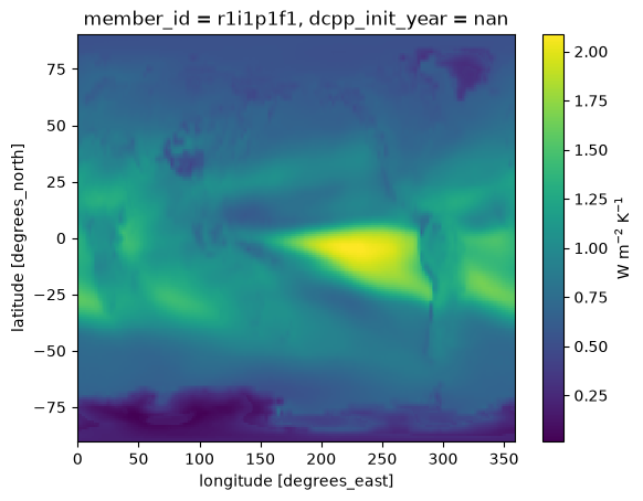
gm_lwq_feedback = global_average(lwq_feedback.mean(dim='month')).load()
gm_lwq_feedbackCould not determine bucket type for bucket name cmip6: Your default credentials were not found. To set up Application Default Credentials, see https://cloud.google.com/docs/authentication/external/set-up-adc for more information., falling back to GCSFileSystem
Could not determine bucket type for bucket name cmip6: Your default credentials were not found. To set up Application Default Credentials, see https://cloud.google.com/docs/authentication/external/set-up-adc for more information., falling back to GCSFileSystem
Could not determine bucket type for bucket name cmip6: Your default credentials were not found. To set up Application Default Credentials, see https://cloud.google.com/docs/authentication/external/set-up-adc for more information., falling back to GCSFileSystem
Could not determine bucket type for bucket name cmip6: Your default credentials were not found. To set up Application Default Credentials, see https://cloud.google.com/docs/authentication/external/set-up-adc for more information., falling back to GCSFileSystem
Could not determine bucket type for bucket name cmip6: Your default credentials were not found. To set up Application Default Credentials, see https://cloud.google.com/docs/authentication/external/set-up-adc for more information., falling back to GCSFileSystem
Could not determine bucket type for bucket name cmip6: Your default credentials were not found. To set up Application Default Credentials, see https://cloud.google.com/docs/authentication/external/set-up-adc for more information., falling back to GCSFileSystem
Could not determine bucket type for bucket name cmip6: Your default credentials were not found. To set up Application Default Credentials, see https://cloud.google.com/docs/authentication/external/set-up-adc for more information., falling back to GCSFileSystem
Could not determine bucket type for bucket name cmip6: Your default credentials were not found. To set up Application Default Credentials, see https://cloud.google.com/docs/authentication/external/set-up-adc for more information., falling back to GCSFileSystem
Could not determine bucket type for bucket name cmip6: Your default credentials were not found. To set up Application Default Credentials, see https://cloud.google.com/docs/authentication/external/set-up-adc for more information., falling back to GCSFileSystem
Could not determine bucket type for bucket name cmip6: Your default credentials were not found. To set up Application Default Credentials, see https://cloud.google.com/docs/authentication/external/set-up-adc for more information., falling back to GCSFileSystem
Could not determine bucket type for bucket name cmip6: Your default credentials were not found. To set up Application Default Credentials, see https://cloud.google.com/docs/authentication/external/set-up-adc for more information., falling back to GCSFileSystem
Could not determine bucket type for bucket name cmip6: Your default credentials were not found. To set up Application Default Credentials, see https://cloud.google.com/docs/authentication/external/set-up-adc for more information., falling back to GCSFileSystem
Could not determine bucket type for bucket name cmip6: Your default credentials were not found. To set up Application Default Credentials, see https://cloud.google.com/docs/authentication/external/set-up-adc for more information., falling back to GCSFileSystem
Could not determine bucket type for bucket name cmip6: Your default credentials were not found. To set up Application Default Credentials, see https://cloud.google.com/docs/authentication/external/set-up-adc for more information., falling back to GCSFileSystem
Could not determine bucket type for bucket name cmip6: Your default credentials were not found. To set up Application Default Credentials, see https://cloud.google.com/docs/authentication/external/set-up-adc for more information., falling back to GCSFileSystem
Could not determine bucket type for bucket name cmip6: Your default credentials were not found. To set up Application Default Credentials, see https://cloud.google.com/docs/authentication/external/set-up-adc for more information., falling back to GCSFileSystem
Could not determine bucket type for bucket name cmip6: Your default credentials were not found. To set up Application Default Credentials, see https://cloud.google.com/docs/authentication/external/set-up-adc for more information., falling back to GCSFileSystem
Could not determine bucket type for bucket name cmip6: Your default credentials were not found. To set up Application Default Credentials, see https://cloud.google.com/docs/authentication/external/set-up-adc for more information., falling back to GCSFileSystem
Could not determine bucket type for bucket name cmip6: Your default credentials were not found. To set up Application Default Credentials, see https://cloud.google.com/docs/authentication/external/set-up-adc for more information., falling back to GCSFileSystem
Could not determine bucket type for bucket name cmip6: Your default credentials were not found. To set up Application Default Credentials, see https://cloud.google.com/docs/authentication/external/set-up-adc for more information., falling back to GCSFileSystem
Could not determine bucket type for bucket name cmip6: Your default credentials were not found. To set up Application Default Credentials, see https://cloud.google.com/docs/authentication/external/set-up-adc for more information., falling back to GCSFileSystem
Could not determine bucket type for bucket name cmip6: Your default credentials were not found. To set up Application Default Credentials, see https://cloud.google.com/docs/authentication/external/set-up-adc for more information., falling back to GCSFileSystem
Could not determine bucket type for bucket name cmip6: Your default credentials were not found. To set up Application Default Credentials, see https://cloud.google.com/docs/authentication/external/set-up-adc for more information., falling back to GCSFileSystem
Could not determine bucket type for bucket name cmip6: Your default credentials were not found. To set up Application Default Credentials, see https://cloud.google.com/docs/authentication/external/set-up-adc for more information., falling back to GCSFileSystem
Could not determine bucket type for bucket name cmip6: Your default credentials were not found. To set up Application Default Credentials, see https://cloud.google.com/docs/authentication/external/set-up-adc for more information., falling back to GCSFileSystem
Could not determine bucket type for bucket name cmip6: Your default credentials were not found. To set up Application Default Credentials, see https://cloud.google.com/docs/authentication/external/set-up-adc for more information., falling back to GCSFileSystem
Could not determine bucket type for bucket name cmip6: Your default credentials were not found. To set up Application Default Credentials, see https://cloud.google.com/docs/authentication/external/set-up-adc for more information., falling back to GCSFileSystem
Could not determine bucket type for bucket name cmip6: Your default credentials were not found. To set up Application Default Credentials, see https://cloud.google.com/docs/authentication/external/set-up-adc for more information., falling back to GCSFileSystem
Could not determine bucket type for bucket name cmip6: Your default credentials were not found. To set up Application Default Credentials, see https://cloud.google.com/docs/authentication/external/set-up-adc for more information., falling back to GCSFileSystem
Could not determine bucket type for bucket name cmip6: Your default credentials were not found. To set up Application Default Credentials, see https://cloud.google.com/docs/authentication/external/set-up-adc for more information., falling back to GCSFileSystem
Could not determine bucket type for bucket name cmip6: Your default credentials were not found. To set up Application Default Credentials, see https://cloud.google.com/docs/authentication/external/set-up-adc for more information., falling back to GCSFileSystem
Could not determine bucket type for bucket name cmip6: Your default credentials were not found. To set up Application Default Credentials, see https://cloud.google.com/docs/authentication/external/set-up-adc for more information., falling back to GCSFileSystem
Could not determine bucket type for bucket name cmip6: Your default credentials were not found. To set up Application Default Credentials, see https://cloud.google.com/docs/authentication/external/set-up-adc for more information., falling back to GCSFileSystem
Could not determine bucket type for bucket name cmip6: Your default credentials were not found. To set up Application Default Credentials, see https://cloud.google.com/docs/authentication/external/set-up-adc for more information., falling back to GCSFileSystem
Could not determine bucket type for bucket name cmip6: Your default credentials were not found. To set up Application Default Credentials, see https://cloud.google.com/docs/authentication/external/set-up-adc for more information., falling back to GCSFileSystem
Could not determine bucket type for bucket name cmip6: Your default credentials were not found. To set up Application Default Credentials, see https://cloud.google.com/docs/authentication/external/set-up-adc for more information., falling back to GCSFileSystem
Could not determine bucket type for bucket name cmip6: Your default credentials were not found. To set up Application Default Credentials, see https://cloud.google.com/docs/authentication/external/set-up-adc for more information., falling back to GCSFileSystem
Could not determine bucket type for bucket name cmip6: Your default credentials were not found. To set up Application Default Credentials, see https://cloud.google.com/docs/authentication/external/set-up-adc for more information., falling back to GCSFileSystem
Could not determine bucket type for bucket name cmip6: Your default credentials were not found. To set up Application Default Credentials, see https://cloud.google.com/docs/authentication/external/set-up-adc for more information., falling back to GCSFileSystem
Could not determine bucket type for bucket name cmip6: Your default credentials were not found. To set up Application Default Credentials, see https://cloud.google.com/docs/authentication/external/set-up-adc for more information., falling back to GCSFileSystem
Could not determine bucket type for bucket name cmip6: Your default credentials were not found. To set up Application Default Credentials, see https://cloud.google.com/docs/authentication/external/set-up-adc for more information., falling back to GCSFileSystem
Could not determine bucket type for bucket name cmip6: Your default credentials were not found. To set up Application Default Credentials, see https://cloud.google.com/docs/authentication/external/set-up-adc for more information., falling back to GCSFileSystem
Could not determine bucket type for bucket name cmip6: Your default credentials were not found. To set up Application Default Credentials, see https://cloud.google.com/docs/authentication/external/set-up-adc for more information., falling back to GCSFileSystem
Could not determine bucket type for bucket name cmip6: Your default credentials were not found. To set up Application Default Credentials, see https://cloud.google.com/docs/authentication/external/set-up-adc for more information., falling back to GCSFileSystem
Could not determine bucket type for bucket name cmip6: Your default credentials were not found. To set up Application Default Credentials, see https://cloud.google.com/docs/authentication/external/set-up-adc for more information., falling back to GCSFileSystem
Could not determine bucket type for bucket name cmip6: Your default credentials were not found. To set up Application Default Credentials, see https://cloud.google.com/docs/authentication/external/set-up-adc for more information., falling back to GCSFileSystem
Could not determine bucket type for bucket name cmip6: Your default credentials were not found. To set up Application Default Credentials, see https://cloud.google.com/docs/authentication/external/set-up-adc for more information., falling back to GCSFileSystem
Could not determine bucket type for bucket name cmip6: Your default credentials were not found. To set up Application Default Credentials, see https://cloud.google.com/docs/authentication/external/set-up-adc for more information., falling back to GCSFileSystem
Could not determine bucket type for bucket name cmip6: Your default credentials were not found. To set up Application Default Credentials, see https://cloud.google.com/docs/authentication/external/set-up-adc for more information., falling back to GCSFileSystem
Could not determine bucket type for bucket name cmip6: Your default credentials were not found. To set up Application Default Credentials, see https://cloud.google.com/docs/authentication/external/set-up-adc for more information., falling back to GCSFileSystem
Could not determine bucket type for bucket name cmip6: Your default credentials were not found. To set up Application Default Credentials, see https://cloud.google.com/docs/authentication/external/set-up-adc for more information., falling back to GCSFileSystem
Could not determine bucket type for bucket name cmip6: Your default credentials were not found. To set up Application Default Credentials, see https://cloud.google.com/docs/authentication/external/set-up-adc for more information., falling back to GCSFileSystem
Could not determine bucket type for bucket name cmip6: Your default credentials were not found. To set up Application Default Credentials, see https://cloud.google.com/docs/authentication/external/set-up-adc for more information., falling back to GCSFileSystem
Could not determine bucket type for bucket name cmip6: Your default credentials were not found. To set up Application Default Credentials, see https://cloud.google.com/docs/authentication/external/set-up-adc for more information., falling back to GCSFileSystem
Could not determine bucket type for bucket name cmip6: Your default credentials were not found. To set up Application Default Credentials, see https://cloud.google.com/docs/authentication/external/set-up-adc for more information., falling back to GCSFileSystem
Could not determine bucket type for bucket name cmip6: Your default credentials were not found. To set up Application Default Credentials, see https://cloud.google.com/docs/authentication/external/set-up-adc for more information., falling back to GCSFileSystem
Could not determine bucket type for bucket name cmip6: Your default credentials were not found. To set up Application Default Credentials, see https://cloud.google.com/docs/authentication/external/set-up-adc for more information., falling back to GCSFileSystem
Could not determine bucket type for bucket name cmip6: Your default credentials were not found. To set up Application Default Credentials, see https://cloud.google.com/docs/authentication/external/set-up-adc for more information., falling back to GCSFileSystem
Could not determine bucket type for bucket name cmip6: Your default credentials were not found. To set up Application Default Credentials, see https://cloud.google.com/docs/authentication/external/set-up-adc for more information., falling back to GCSFileSystem
Could not determine bucket type for bucket name cmip6: Your default credentials were not found. To set up Application Default Credentials, see https://cloud.google.com/docs/authentication/external/set-up-adc for more information., falling back to GCSFileSystem
Could not determine bucket type for bucket name cmip6: Your default credentials were not found. To set up Application Default Credentials, see https://cloud.google.com/docs/authentication/external/set-up-adc for more information., falling back to GCSFileSystem
Could not determine bucket type for bucket name cmip6: Your default credentials were not found. To set up Application Default Credentials, see https://cloud.google.com/docs/authentication/external/set-up-adc for more information., falling back to GCSFileSystem
Could not determine bucket type for bucket name cmip6: Your default credentials were not found. To set up Application Default Credentials, see https://cloud.google.com/docs/authentication/external/set-up-adc for more information., falling back to GCSFileSystem
Could not determine bucket type for bucket name cmip6: Your default credentials were not found. To set up Application Default Credentials, see https://cloud.google.com/docs/authentication/external/set-up-adc for more information., falling back to GCSFileSystem
Could not determine bucket type for bucket name cmip6: Your default credentials were not found. To set up Application Default Credentials, see https://cloud.google.com/docs/authentication/external/set-up-adc for more information., falling back to GCSFileSystem
Could not determine bucket type for bucket name cmip6: Your default credentials were not found. To set up Application Default Credentials, see https://cloud.google.com/docs/authentication/external/set-up-adc for more information., falling back to GCSFileSystem
Could not determine bucket type for bucket name cmip6: Your default credentials were not found. To set up Application Default Credentials, see https://cloud.google.com/docs/authentication/external/set-up-adc for more information., falling back to GCSFileSystem
Could not determine bucket type for bucket name cmip6: Your default credentials were not found. To set up Application Default Credentials, see https://cloud.google.com/docs/authentication/external/set-up-adc for more information., falling back to GCSFileSystem
Could not determine bucket type for bucket name cmip6: Your default credentials were not found. To set up Application Default Credentials, see https://cloud.google.com/docs/authentication/external/set-up-adc for more information., falling back to GCSFileSystem
Could not determine bucket type for bucket name cmip6: Your default credentials were not found. To set up Application Default Credentials, see https://cloud.google.com/docs/authentication/external/set-up-adc for more information., falling back to GCSFileSystem
Could not determine bucket type for bucket name cmip6: Your default credentials were not found. To set up Application Default Credentials, see https://cloud.google.com/docs/authentication/external/set-up-adc for more information., falling back to GCSFileSystem
Could not determine bucket type for bucket name cmip6: Your default credentials were not found. To set up Application Default Credentials, see https://cloud.google.com/docs/authentication/external/set-up-adc for more information., falling back to GCSFileSystem
Could not determine bucket type for bucket name cmip6: Your default credentials were not found. To set up Application Default Credentials, see https://cloud.google.com/docs/authentication/external/set-up-adc for more information., falling back to GCSFileSystem
Could not determine bucket type for bucket name cmip6: Your default credentials were not found. To set up Application Default Credentials, see https://cloud.google.com/docs/authentication/external/set-up-adc for more information., falling back to GCSFileSystem
Could not determine bucket type for bucket name cmip6: Your default credentials were not found. To set up Application Default Credentials, see https://cloud.google.com/docs/authentication/external/set-up-adc for more information., falling back to GCSFileSystem
Could not determine bucket type for bucket name cmip6: Your default credentials were not found. To set up Application Default Credentials, see https://cloud.google.com/docs/authentication/external/set-up-adc for more information., falling back to GCSFileSystem
Could not determine bucket type for bucket name cmip6: Your default credentials were not found. To set up Application Default Credentials, see https://cloud.google.com/docs/authentication/external/set-up-adc for more information., falling back to GCSFileSystem
Could not determine bucket type for bucket name cmip6: Your default credentials were not found. To set up Application Default Credentials, see https://cloud.google.com/docs/authentication/external/set-up-adc for more information., falling back to GCSFileSystem
Could not determine bucket type for bucket name cmip6: Your default credentials were not found. To set up Application Default Credentials, see https://cloud.google.com/docs/authentication/external/set-up-adc for more information., falling back to GCSFileSystem
Could not determine bucket type for bucket name cmip6: Your default credentials were not found. To set up Application Default Credentials, see https://cloud.google.com/docs/authentication/external/set-up-adc for more information., falling back to GCSFileSystem
Could not determine bucket type for bucket name cmip6: Your default credentials were not found. To set up Application Default Credentials, see https://cloud.google.com/docs/authentication/external/set-up-adc for more information., falling back to GCSFileSystem
Could not determine bucket type for bucket name cmip6: Your default credentials were not found. To set up Application Default Credentials, see https://cloud.google.com/docs/authentication/external/set-up-adc for more information., falling back to GCSFileSystem
Could not determine bucket type for bucket name cmip6: Your default credentials were not found. To set up Application Default Credentials, see https://cloud.google.com/docs/authentication/external/set-up-adc for more information., falling back to GCSFileSystem
Could not determine bucket type for bucket name cmip6: Your default credentials were not found. To set up Application Default Credentials, see https://cloud.google.com/docs/authentication/external/set-up-adc for more information., falling back to GCSFileSystem
Could not determine bucket type for bucket name cmip6: Your default credentials were not found. To set up Application Default Credentials, see https://cloud.google.com/docs/authentication/external/set-up-adc for more information., falling back to GCSFileSystem
Could not determine bucket type for bucket name cmip6: Your default credentials were not found. To set up Application Default Credentials, see https://cloud.google.com/docs/authentication/external/set-up-adc for more information., falling back to GCSFileSystem
Could not determine bucket type for bucket name cmip6: Your default credentials were not found. To set up Application Default Credentials, see https://cloud.google.com/docs/authentication/external/set-up-adc for more information., falling back to GCSFileSystem
Could not determine bucket type for bucket name cmip6: Your default credentials were not found. To set up Application Default Credentials, see https://cloud.google.com/docs/authentication/external/set-up-adc for more information., falling back to GCSFileSystem
Could not determine bucket type for bucket name cmip6: Your default credentials were not found. To set up Application Default Credentials, see https://cloud.google.com/docs/authentication/external/set-up-adc for more information., falling back to GCSFileSystem
Could not determine bucket type for bucket name cmip6: Your default credentials were not found. To set up Application Default Credentials, see https://cloud.google.com/docs/authentication/external/set-up-adc for more information., falling back to GCSFileSystem
Could not determine bucket type for bucket name cmip6: Your default credentials were not found. To set up Application Default Credentials, see https://cloud.google.com/docs/authentication/external/set-up-adc for more information., falling back to GCSFileSystem
Could not determine bucket type for bucket name cmip6: Your default credentials were not found. To set up Application Default Credentials, see https://cloud.google.com/docs/authentication/external/set-up-adc for more information., falling back to GCSFileSystem
Could not determine bucket type for bucket name cmip6: Your default credentials were not found. To set up Application Default Credentials, see https://cloud.google.com/docs/authentication/external/set-up-adc for more information., falling back to GCSFileSystem
Could not determine bucket type for bucket name cmip6: Your default credentials were not found. To set up Application Default Credentials, see https://cloud.google.com/docs/authentication/external/set-up-adc for more information., falling back to GCSFileSystem
Could not determine bucket type for bucket name cmip6: Your default credentials were not found. To set up Application Default Credentials, see https://cloud.google.com/docs/authentication/external/set-up-adc for more information., falling back to GCSFileSystem
Could not determine bucket type for bucket name cmip6: Your default credentials were not found. To set up Application Default Credentials, see https://cloud.google.com/docs/authentication/external/set-up-adc for more information., falling back to GCSFileSystem
Could not determine bucket type for bucket name cmip6: Your default credentials were not found. To set up Application Default Credentials, see https://cloud.google.com/docs/authentication/external/set-up-adc for more information., falling back to GCSFileSystem
Could not determine bucket type for bucket name cmip6: Your default credentials were not found. To set up Application Default Credentials, see https://cloud.google.com/docs/authentication/external/set-up-adc for more information., falling back to GCSFileSystem
Could not determine bucket type for bucket name cmip6: Your default credentials were not found. To set up Application Default Credentials, see https://cloud.google.com/docs/authentication/external/set-up-adc for more information., falling back to GCSFileSystem
Could not determine bucket type for bucket name cmip6: Your default credentials were not found. To set up Application Default Credentials, see https://cloud.google.com/docs/authentication/external/set-up-adc for more information., falling back to GCSFileSystem
Could not determine bucket type for bucket name cmip6: Your default credentials were not found. To set up Application Default Credentials, see https://cloud.google.com/docs/authentication/external/set-up-adc for more information., falling back to GCSFileSystem
Could not determine bucket type for bucket name cmip6: Your default credentials were not found. To set up Application Default Credentials, see https://cloud.google.com/docs/authentication/external/set-up-adc for more information., falling back to GCSFileSystem
Could not determine bucket type for bucket name cmip6: Your default credentials were not found. To set up Application Default Credentials, see https://cloud.google.com/docs/authentication/external/set-up-adc for more information., falling back to GCSFileSystem
Could not determine bucket type for bucket name cmip6: Your default credentials were not found. To set up Application Default Credentials, see https://cloud.google.com/docs/authentication/external/set-up-adc for more information., falling back to GCSFileSystem
Could not determine bucket type for bucket name cmip6: Your default credentials were not found. To set up Application Default Credentials, see https://cloud.google.com/docs/authentication/external/set-up-adc for more information., falling back to GCSFileSystem
Could not determine bucket type for bucket name cmip6: Your default credentials were not found. To set up Application Default Credentials, see https://cloud.google.com/docs/authentication/external/set-up-adc for more information., falling back to GCSFileSystem
Could not determine bucket type for bucket name cmip6: Your default credentials were not found. To set up Application Default Credentials, see https://cloud.google.com/docs/authentication/external/set-up-adc for more information., falling back to GCSFileSystem
Could not determine bucket type for bucket name cmip6: Your default credentials were not found. To set up Application Default Credentials, see https://cloud.google.com/docs/authentication/external/set-up-adc for more information., falling back to GCSFileSystem
Could not determine bucket type for bucket name cmip6: Your default credentials were not found. To set up Application Default Credentials, see https://cloud.google.com/docs/authentication/external/set-up-adc for more information., falling back to GCSFileSystem
Could not determine bucket type for bucket name cmip6: Your default credentials were not found. To set up Application Default Credentials, see https://cloud.google.com/docs/authentication/external/set-up-adc for more information., falling back to GCSFileSystem
Could not determine bucket type for bucket name cmip6: Your default credentials were not found. To set up Application Default Credentials, see https://cloud.google.com/docs/authentication/external/set-up-adc for more information., falling back to GCSFileSystem
Could not determine bucket type for bucket name cmip6: Your default credentials were not found. To set up Application Default Credentials, see https://cloud.google.com/docs/authentication/external/set-up-adc for more information., falling back to GCSFileSystem
Could not determine bucket type for bucket name cmip6: Your default credentials were not found. To set up Application Default Credentials, see https://cloud.google.com/docs/authentication/external/set-up-adc for more information., falling back to GCSFileSystem
Could not determine bucket type for bucket name cmip6: Your default credentials were not found. To set up Application Default Credentials, see https://cloud.google.com/docs/authentication/external/set-up-adc for more information., falling back to GCSFileSystem
Could not determine bucket type for bucket name cmip6: Your default credentials were not found. To set up Application Default Credentials, see https://cloud.google.com/docs/authentication/external/set-up-adc for more information., falling back to GCSFileSystem
Could not determine bucket type for bucket name cmip6: Your default credentials were not found. To set up Application Default Credentials, see https://cloud.google.com/docs/authentication/external/set-up-adc for more information., falling back to GCSFileSystem
Could not determine bucket type for bucket name cmip6: Your default credentials were not found. To set up Application Default Credentials, see https://cloud.google.com/docs/authentication/external/set-up-adc for more information., falling back to GCSFileSystem
Could not determine bucket type for bucket name cmip6: Your default credentials were not found. To set up Application Default Credentials, see https://cloud.google.com/docs/authentication/external/set-up-adc for more information., falling back to GCSFileSystem
Could not determine bucket type for bucket name cmip6: Your default credentials were not found. To set up Application Default Credentials, see https://cloud.google.com/docs/authentication/external/set-up-adc for more information., falling back to GCSFileSystem
Could not determine bucket type for bucket name cmip6: Your default credentials were not found. To set up Application Default Credentials, see https://cloud.google.com/docs/authentication/external/set-up-adc for more information., falling back to GCSFileSystem
Could not determine bucket type for bucket name cmip6: Your default credentials were not found. To set up Application Default Credentials, see https://cloud.google.com/docs/authentication/external/set-up-adc for more information., falling back to GCSFileSystem
Could not determine bucket type for bucket name cmip6: Your default credentials were not found. To set up Application Default Credentials, see https://cloud.google.com/docs/authentication/external/set-up-adc for more information., falling back to GCSFileSystem
Could not determine bucket type for bucket name cmip6: Your default credentials were not found. To set up Application Default Credentials, see https://cloud.google.com/docs/authentication/external/set-up-adc for more information., falling back to GCSFileSystem
Could not determine bucket type for bucket name cmip6: Your default credentials were not found. To set up Application Default Credentials, see https://cloud.google.com/docs/authentication/external/set-up-adc for more information., falling back to GCSFileSystem
Could not determine bucket type for bucket name cmip6: Your default credentials were not found. To set up Application Default Credentials, see https://cloud.google.com/docs/authentication/external/set-up-adc for more information., falling back to GCSFileSystem
Could not determine bucket type for bucket name cmip6: Your default credentials were not found. To set up Application Default Credentials, see https://cloud.google.com/docs/authentication/external/set-up-adc for more information., falling back to GCSFileSystem
Could not determine bucket type for bucket name cmip6: Your default credentials were not found. To set up Application Default Credentials, see https://cloud.google.com/docs/authentication/external/set-up-adc for more information., falling back to GCSFileSystem
Could not determine bucket type for bucket name cmip6: Your default credentials were not found. To set up Application Default Credentials, see https://cloud.google.com/docs/authentication/external/set-up-adc for more information., falling back to GCSFileSystem
Could not determine bucket type for bucket name cmip6: Your default credentials were not found. To set up Application Default Credentials, see https://cloud.google.com/docs/authentication/external/set-up-adc for more information., falling back to GCSFileSystem
Could not determine bucket type for bucket name cmip6: Your default credentials were not found. To set up Application Default Credentials, see https://cloud.google.com/docs/authentication/external/set-up-adc for more information., falling back to GCSFileSystem
Could not determine bucket type for bucket name cmip6: Your default credentials were not found. To set up Application Default Credentials, see https://cloud.google.com/docs/authentication/external/set-up-adc for more information., falling back to GCSFileSystem
Could not determine bucket type for bucket name cmip6: Your default credentials were not found. To set up Application Default Credentials, see https://cloud.google.com/docs/authentication/external/set-up-adc for more information., falling back to GCSFileSystem
Could not determine bucket type for bucket name cmip6: Your default credentials were not found. To set up Application Default Credentials, see https://cloud.google.com/docs/authentication/external/set-up-adc for more information., falling back to GCSFileSystem
Could not determine bucket type for bucket name cmip6: Your default credentials were not found. To set up Application Default Credentials, see https://cloud.google.com/docs/authentication/external/set-up-adc for more information., falling back to GCSFileSystem
Could not determine bucket type for bucket name cmip6: Your default credentials were not found. To set up Application Default Credentials, see https://cloud.google.com/docs/authentication/external/set-up-adc for more information., falling back to GCSFileSystem
Could not determine bucket type for bucket name cmip6: Your default credentials were not found. To set up Application Default Credentials, see https://cloud.google.com/docs/authentication/external/set-up-adc for more information., falling back to GCSFileSystem
Could not determine bucket type for bucket name cmip6: Your default credentials were not found. To set up Application Default Credentials, see https://cloud.google.com/docs/authentication/external/set-up-adc for more information., falling back to GCSFileSystem
Could not determine bucket type for bucket name cmip6: Your default credentials were not found. To set up Application Default Credentials, see https://cloud.google.com/docs/authentication/external/set-up-adc for more information., falling back to GCSFileSystem
Could not determine bucket type for bucket name cmip6: Your default credentials were not found. To set up Application Default Credentials, see https://cloud.google.com/docs/authentication/external/set-up-adc for more information., falling back to GCSFileSystem
Could not determine bucket type for bucket name cmip6: Your default credentials were not found. To set up Application Default Credentials, see https://cloud.google.com/docs/authentication/external/set-up-adc for more information., falling back to GCSFileSystem
Could not determine bucket type for bucket name cmip6: Your default credentials were not found. To set up Application Default Credentials, see https://cloud.google.com/docs/authentication/external/set-up-adc for more information., falling back to GCSFileSystem
Could not determine bucket type for bucket name cmip6: Your default credentials were not found. To set up Application Default Credentials, see https://cloud.google.com/docs/authentication/external/set-up-adc for more information., falling back to GCSFileSystem
Could not determine bucket type for bucket name cmip6: Your default credentials were not found. To set up Application Default Credentials, see https://cloud.google.com/docs/authentication/external/set-up-adc for more information., falling back to GCSFileSystem
Could not determine bucket type for bucket name cmip6: Your default credentials were not found. To set up Application Default Credentials, see https://cloud.google.com/docs/authentication/external/set-up-adc for more information., falling back to GCSFileSystem
Could not determine bucket type for bucket name cmip6: Your default credentials were not found. To set up Application Default Credentials, see https://cloud.google.com/docs/authentication/external/set-up-adc for more information., falling back to GCSFileSystem
Could not determine bucket type for bucket name cmip6: Your default credentials were not found. To set up Application Default Credentials, see https://cloud.google.com/docs/authentication/external/set-up-adc for more information., falling back to GCSFileSystem
Could not determine bucket type for bucket name cmip6: Your default credentials were not found. To set up Application Default Credentials, see https://cloud.google.com/docs/authentication/external/set-up-adc for more information., falling back to GCSFileSystem
Could not determine bucket type for bucket name cmip6: Your default credentials were not found. To set up Application Default Credentials, see https://cloud.google.com/docs/authentication/external/set-up-adc for more information., falling back to GCSFileSystem
Could not determine bucket type for bucket name cmip6: Your default credentials were not found. To set up Application Default Credentials, see https://cloud.google.com/docs/authentication/external/set-up-adc for more information., falling back to GCSFileSystem
Could not determine bucket type for bucket name cmip6: Your default credentials were not found. To set up Application Default Credentials, see https://cloud.google.com/docs/authentication/external/set-up-adc for more information., falling back to GCSFileSystem
Could not determine bucket type for bucket name cmip6: Your default credentials were not found. To set up Application Default Credentials, see https://cloud.google.com/docs/authentication/external/set-up-adc for more information., falling back to GCSFileSystem
Could not determine bucket type for bucket name cmip6: Your default credentials were not found. To set up Application Default Credentials, see https://cloud.google.com/docs/authentication/external/set-up-adc for more information., falling back to GCSFileSystem
Could not determine bucket type for bucket name cmip6: Your default credentials were not found. To set up Application Default Credentials, see https://cloud.google.com/docs/authentication/external/set-up-adc for more information., falling back to GCSFileSystem
Could not determine bucket type for bucket name cmip6: Your default credentials were not found. To set up Application Default Credentials, see https://cloud.google.com/docs/authentication/external/set-up-adc for more information., falling back to GCSFileSystem
Could not determine bucket type for bucket name cmip6: Your default credentials were not found. To set up Application Default Credentials, see https://cloud.google.com/docs/authentication/external/set-up-adc for more information., falling back to GCSFileSystem
Could not determine bucket type for bucket name cmip6: Your default credentials were not found. To set up Application Default Credentials, see https://cloud.google.com/docs/authentication/external/set-up-adc for more information., falling back to GCSFileSystem
Could not determine bucket type for bucket name cmip6: Your default credentials were not found. To set up Application Default Credentials, see https://cloud.google.com/docs/authentication/external/set-up-adc for more information., falling back to GCSFileSystem
Could not determine bucket type for bucket name cmip6: Your default credentials were not found. To set up Application Default Credentials, see https://cloud.google.com/docs/authentication/external/set-up-adc for more information., falling back to GCSFileSystem
Could not determine bucket type for bucket name cmip6: Your default credentials were not found. To set up Application Default Credentials, see https://cloud.google.com/docs/authentication/external/set-up-adc for more information., falling back to GCSFileSystem
Could not determine bucket type for bucket name cmip6: Your default credentials were not found. To set up Application Default Credentials, see https://cloud.google.com/docs/authentication/external/set-up-adc for more information., falling back to GCSFileSystem
Could not determine bucket type for bucket name cmip6: Your default credentials were not found. To set up Application Default Credentials, see https://cloud.google.com/docs/authentication/external/set-up-adc for more information., falling back to GCSFileSystem
Could not determine bucket type for bucket name cmip6: Your default credentials were not found. To set up Application Default Credentials, see https://cloud.google.com/docs/authentication/external/set-up-adc for more information., falling back to GCSFileSystem
Could not determine bucket type for bucket name cmip6: Your default credentials were not found. To set up Application Default Credentials, see https://cloud.google.com/docs/authentication/external/set-up-adc for more information., falling back to GCSFileSystem
Could not determine bucket type for bucket name cmip6: Your default credentials were not found. To set up Application Default Credentials, see https://cloud.google.com/docs/authentication/external/set-up-adc for more information., falling back to GCSFileSystem
Could not determine bucket type for bucket name cmip6: Your default credentials were not found. To set up Application Default Credentials, see https://cloud.google.com/docs/authentication/external/set-up-adc for more information., falling back to GCSFileSystem
Could not determine bucket type for bucket name cmip6: Your default credentials were not found. To set up Application Default Credentials, see https://cloud.google.com/docs/authentication/external/set-up-adc for more information., falling back to GCSFileSystem
Could not determine bucket type for bucket name cmip6: Your default credentials were not found. To set up Application Default Credentials, see https://cloud.google.com/docs/authentication/external/set-up-adc for more information., falling back to GCSFileSystem
Could not determine bucket type for bucket name cmip6: Your default credentials were not found. To set up Application Default Credentials, see https://cloud.google.com/docs/authentication/external/set-up-adc for more information., falling back to GCSFileSystem
Could not determine bucket type for bucket name cmip6: Your default credentials were not found. To set up Application Default Credentials, see https://cloud.google.com/docs/authentication/external/set-up-adc for more information., falling back to GCSFileSystem
Could not determine bucket type for bucket name cmip6: Your default credentials were not found. To set up Application Default Credentials, see https://cloud.google.com/docs/authentication/external/set-up-adc for more information., falling back to GCSFileSystem
Could not determine bucket type for bucket name cmip6: Your default credentials were not found. To set up Application Default Credentials, see https://cloud.google.com/docs/authentication/external/set-up-adc for more information., falling back to GCSFileSystem
Could not determine bucket type for bucket name cmip6: Your default credentials were not found. To set up Application Default Credentials, see https://cloud.google.com/docs/authentication/external/set-up-adc for more information., falling back to GCSFileSystem
Could not determine bucket type for bucket name cmip6: Your default credentials were not found. To set up Application Default Credentials, see https://cloud.google.com/docs/authentication/external/set-up-adc for more information., falling back to GCSFileSystem
Could not determine bucket type for bucket name cmip6: Your default credentials were not found. To set up Application Default Credentials, see https://cloud.google.com/docs/authentication/external/set-up-adc for more information., falling back to GCSFileSystem
Could not determine bucket type for bucket name cmip6: Your default credentials were not found. To set up Application Default Credentials, see https://cloud.google.com/docs/authentication/external/set-up-adc for more information., falling back to GCSFileSystem
Could not determine bucket type for bucket name cmip6: Your default credentials were not found. To set up Application Default Credentials, see https://cloud.google.com/docs/authentication/external/set-up-adc for more information., falling back to GCSFileSystem
Could not determine bucket type for bucket name cmip6: Your default credentials were not found. To set up Application Default Credentials, see https://cloud.google.com/docs/authentication/external/set-up-adc for more information., falling back to GCSFileSystem
Could not determine bucket type for bucket name cmip6: Your default credentials were not found. To set up Application Default Credentials, see https://cloud.google.com/docs/authentication/external/set-up-adc for more information., falling back to GCSFileSystem
Could not determine bucket type for bucket name cmip6: Your default credentials were not found. To set up Application Default Credentials, see https://cloud.google.com/docs/authentication/external/set-up-adc for more information., falling back to GCSFileSystem
Could not determine bucket type for bucket name cmip6: Your default credentials were not found. To set up Application Default Credentials, see https://cloud.google.com/docs/authentication/external/set-up-adc for more information., falling back to GCSFileSystem
Could not determine bucket type for bucket name cmip6: Your default credentials were not found. To set up Application Default Credentials, see https://cloud.google.com/docs/authentication/external/set-up-adc for more information., falling back to GCSFileSystem
Could not determine bucket type for bucket name cmip6: Your default credentials were not found. To set up Application Default Credentials, see https://cloud.google.com/docs/authentication/external/set-up-adc for more information., falling back to GCSFileSystem
Could not determine bucket type for bucket name cmip6: Your default credentials were not found. To set up Application Default Credentials, see https://cloud.google.com/docs/authentication/external/set-up-adc for more information., falling back to GCSFileSystem
Could not determine bucket type for bucket name cmip6: Your default credentials were not found. To set up Application Default Credentials, see https://cloud.google.com/docs/authentication/external/set-up-adc for more information., falling back to GCSFileSystem
Could not determine bucket type for bucket name cmip6: Your default credentials were not found. To set up Application Default Credentials, see https://cloud.google.com/docs/authentication/external/set-up-adc for more information., falling back to GCSFileSystem
Could not determine bucket type for bucket name cmip6: Your default credentials were not found. To set up Application Default Credentials, see https://cloud.google.com/docs/authentication/external/set-up-adc for more information., falling back to GCSFileSystem
Could not determine bucket type for bucket name cmip6: Your default credentials were not found. To set up Application Default Credentials, see https://cloud.google.com/docs/authentication/external/set-up-adc for more information., falling back to GCSFileSystem
Could not determine bucket type for bucket name cmip6: Your default credentials were not found. To set up Application Default Credentials, see https://cloud.google.com/docs/authentication/external/set-up-adc for more information., falling back to GCSFileSystem
Could not determine bucket type for bucket name cmip6: Your default credentials were not found. To set up Application Default Credentials, see https://cloud.google.com/docs/authentication/external/set-up-adc for more information., falling back to GCSFileSystem
Could not determine bucket type for bucket name cmip6: Your default credentials were not found. To set up Application Default Credentials, see https://cloud.google.com/docs/authentication/external/set-up-adc for more information., falling back to GCSFileSystem
Could not determine bucket type for bucket name cmip6: Your default credentials were not found. To set up Application Default Credentials, see https://cloud.google.com/docs/authentication/external/set-up-adc for more information., falling back to GCSFileSystem
Could not determine bucket type for bucket name cmip6: Your default credentials were not found. To set up Application Default Credentials, see https://cloud.google.com/docs/authentication/external/set-up-adc for more information., falling back to GCSFileSystem
Could not determine bucket type for bucket name cmip6: Your default credentials were not found. To set up Application Default Credentials, see https://cloud.google.com/docs/authentication/external/set-up-adc for more information., falling back to GCSFileSystem
Could not determine bucket type for bucket name cmip6: Your default credentials were not found. To set up Application Default Credentials, see https://cloud.google.com/docs/authentication/external/set-up-adc for more information., falling back to GCSFileSystem
Could not determine bucket type for bucket name cmip6: Your default credentials were not found. To set up Application Default Credentials, see https://cloud.google.com/docs/authentication/external/set-up-adc for more information., falling back to GCSFileSystem
Could not determine bucket type for bucket name cmip6: Your default credentials were not found. To set up Application Default Credentials, see https://cloud.google.com/docs/authentication/external/set-up-adc for more information., falling back to GCSFileSystem
Could not determine bucket type for bucket name cmip6: Your default credentials were not found. To set up Application Default Credentials, see https://cloud.google.com/docs/authentication/external/set-up-adc for more information., falling back to GCSFileSystem
Could not determine bucket type for bucket name cmip6: Your default credentials were not found. To set up Application Default Credentials, see https://cloud.google.com/docs/authentication/external/set-up-adc for more information., falling back to GCSFileSystem
Could not determine bucket type for bucket name cmip6: Your default credentials were not found. To set up Application Default Credentials, see https://cloud.google.com/docs/authentication/external/set-up-adc for more information., falling back to GCSFileSystem
Could not determine bucket type for bucket name cmip6: Your default credentials were not found. To set up Application Default Credentials, see https://cloud.google.com/docs/authentication/external/set-up-adc for more information., falling back to GCSFileSystem
Could not determine bucket type for bucket name cmip6: Your default credentials were not found. To set up Application Default Credentials, see https://cloud.google.com/docs/authentication/external/set-up-adc for more information., falling back to GCSFileSystem
Could not determine bucket type for bucket name cmip6: Your default credentials were not found. To set up Application Default Credentials, see https://cloud.google.com/docs/authentication/external/set-up-adc for more information., falling back to GCSFileSystem
Could not determine bucket type for bucket name cmip6: Your default credentials were not found. To set up Application Default Credentials, see https://cloud.google.com/docs/authentication/external/set-up-adc for more information., falling back to GCSFileSystem
Could not determine bucket type for bucket name cmip6: Your default credentials were not found. To set up Application Default Credentials, see https://cloud.google.com/docs/authentication/external/set-up-adc for more information., falling back to GCSFileSystem
Could not determine bucket type for bucket name cmip6: Your default credentials were not found. To set up Application Default Credentials, see https://cloud.google.com/docs/authentication/external/set-up-adc for more information., falling back to GCSFileSystem
Could not determine bucket type for bucket name cmip6: Your default credentials were not found. To set up Application Default Credentials, see https://cloud.google.com/docs/authentication/external/set-up-adc for more information., falling back to GCSFileSystem
Could not determine bucket type for bucket name cmip6: Your default credentials were not found. To set up Application Default Credentials, see https://cloud.google.com/docs/authentication/external/set-up-adc for more information., falling back to GCSFileSystem
Could not determine bucket type for bucket name cmip6: Your default credentials were not found. To set up Application Default Credentials, see https://cloud.google.com/docs/authentication/external/set-up-adc for more information., falling back to GCSFileSystem
Could not determine bucket type for bucket name cmip6: Your default credentials were not found. To set up Application Default Credentials, see https://cloud.google.com/docs/authentication/external/set-up-adc for more information., falling back to GCSFileSystem
Could not determine bucket type for bucket name cmip6: Your default credentials were not found. To set up Application Default Credentials, see https://cloud.google.com/docs/authentication/external/set-up-adc for more information., falling back to GCSFileSystem
Could not determine bucket type for bucket name cmip6: Your default credentials were not found. To set up Application Default Credentials, see https://cloud.google.com/docs/authentication/external/set-up-adc for more information., falling back to GCSFileSystem
Could not determine bucket type for bucket name cmip6: Your default credentials were not found. To set up Application Default Credentials, see https://cloud.google.com/docs/authentication/external/set-up-adc for more information., falling back to GCSFileSystem
Could not determine bucket type for bucket name cmip6: Your default credentials were not found. To set up Application Default Credentials, see https://cloud.google.com/docs/authentication/external/set-up-adc for more information., falling back to GCSFileSystem
Could not determine bucket type for bucket name cmip6: Your default credentials were not found. To set up Application Default Credentials, see https://cloud.google.com/docs/authentication/external/set-up-adc for more information., falling back to GCSFileSystem
Could not determine bucket type for bucket name cmip6: Your default credentials were not found. To set up Application Default Credentials, see https://cloud.google.com/docs/authentication/external/set-up-adc for more information., falling back to GCSFileSystem
Could not determine bucket type for bucket name cmip6: Your default credentials were not found. To set up Application Default Credentials, see https://cloud.google.com/docs/authentication/external/set-up-adc for more information., falling back to GCSFileSystem
Could not determine bucket type for bucket name cmip6: Your default credentials were not found. To set up Application Default Credentials, see https://cloud.google.com/docs/authentication/external/set-up-adc for more information., falling back to GCSFileSystem
Could not determine bucket type for bucket name cmip6: Your default credentials were not found. To set up Application Default Credentials, see https://cloud.google.com/docs/authentication/external/set-up-adc for more information., falling back to GCSFileSystem
Could not determine bucket type for bucket name cmip6: Your default credentials were not found. To set up Application Default Credentials, see https://cloud.google.com/docs/authentication/external/set-up-adc for more information., falling back to GCSFileSystem
Could not determine bucket type for bucket name cmip6: Your default credentials were not found. To set up Application Default Credentials, see https://cloud.google.com/docs/authentication/external/set-up-adc for more information., falling back to GCSFileSystem
Could not determine bucket type for bucket name cmip6: Your default credentials were not found. To set up Application Default Credentials, see https://cloud.google.com/docs/authentication/external/set-up-adc for more information., falling back to GCSFileSystem
Could not determine bucket type for bucket name cmip6: Your default credentials were not found. To set up Application Default Credentials, see https://cloud.google.com/docs/authentication/external/set-up-adc for more information., falling back to GCSFileSystem
Could not determine bucket type for bucket name cmip6: Your default credentials were not found. To set up Application Default Credentials, see https://cloud.google.com/docs/authentication/external/set-up-adc for more information., falling back to GCSFileSystem
Could not determine bucket type for bucket name cmip6: Your default credentials were not found. To set up Application Default Credentials, see https://cloud.google.com/docs/authentication/external/set-up-adc for more information., falling back to GCSFileSystem
Could not determine bucket type for bucket name cmip6: Your default credentials were not found. To set up Application Default Credentials, see https://cloud.google.com/docs/authentication/external/set-up-adc for more information., falling back to GCSFileSystem
Could not determine bucket type for bucket name cmip6: Your default credentials were not found. To set up Application Default Credentials, see https://cloud.google.com/docs/authentication/external/set-up-adc for more information., falling back to GCSFileSystem
Could not determine bucket type for bucket name cmip6: Your default credentials were not found. To set up Application Default Credentials, see https://cloud.google.com/docs/authentication/external/set-up-adc for more information., falling back to GCSFileSystem
Could not determine bucket type for bucket name cmip6: Your default credentials were not found. To set up Application Default Credentials, see https://cloud.google.com/docs/authentication/external/set-up-adc for more information., falling back to GCSFileSystem
Could not determine bucket type for bucket name cmip6: Your default credentials were not found. To set up Application Default Credentials, see https://cloud.google.com/docs/authentication/external/set-up-adc for more information., falling back to GCSFileSystem
Could not determine bucket type for bucket name cmip6: Your default credentials were not found. To set up Application Default Credentials, see https://cloud.google.com/docs/authentication/external/set-up-adc for more information., falling back to GCSFileSystem
Could not determine bucket type for bucket name cmip6: Your default credentials were not found. To set up Application Default Credentials, see https://cloud.google.com/docs/authentication/external/set-up-adc for more information., falling back to GCSFileSystem
Could not determine bucket type for bucket name cmip6: Your default credentials were not found. To set up Application Default Credentials, see https://cloud.google.com/docs/authentication/external/set-up-adc for more information., falling back to GCSFileSystem
Could not determine bucket type for bucket name cmip6: Your default credentials were not found. To set up Application Default Credentials, see https://cloud.google.com/docs/authentication/external/set-up-adc for more information., falling back to GCSFileSystem
Could not determine bucket type for bucket name cmip6: Your default credentials were not found. To set up Application Default Credentials, see https://cloud.google.com/docs/authentication/external/set-up-adc for more information., falling back to GCSFileSystem
Could not determine bucket type for bucket name cmip6: Your default credentials were not found. To set up Application Default Credentials, see https://cloud.google.com/docs/authentication/external/set-up-adc for more information., falling back to GCSFileSystem
Could not determine bucket type for bucket name cmip6: Your default credentials were not found. To set up Application Default Credentials, see https://cloud.google.com/docs/authentication/external/set-up-adc for more information., falling back to GCSFileSystem
Could not determine bucket type for bucket name cmip6: Your default credentials were not found. To set up Application Default Credentials, see https://cloud.google.com/docs/authentication/external/set-up-adc for more information., falling back to GCSFileSystem
Could not determine bucket type for bucket name cmip6: Your default credentials were not found. To set up Application Default Credentials, see https://cloud.google.com/docs/authentication/external/set-up-adc for more information., falling back to GCSFileSystem
Could not determine bucket type for bucket name cmip6: Your default credentials were not found. To set up Application Default Credentials, see https://cloud.google.com/docs/authentication/external/set-up-adc for more information., falling back to GCSFileSystem
Could not determine bucket type for bucket name cmip6: Your default credentials were not found. To set up Application Default Credentials, see https://cloud.google.com/docs/authentication/external/set-up-adc for more information., falling back to GCSFileSystem
Could not determine bucket type for bucket name cmip6: Your default credentials were not found. To set up Application Default Credentials, see https://cloud.google.com/docs/authentication/external/set-up-adc for more information., falling back to GCSFileSystem
Could not determine bucket type for bucket name cmip6: Your default credentials were not found. To set up Application Default Credentials, see https://cloud.google.com/docs/authentication/external/set-up-adc for more information., falling back to GCSFileSystem
Could not determine bucket type for bucket name cmip6: Your default credentials were not found. To set up Application Default Credentials, see https://cloud.google.com/docs/authentication/external/set-up-adc for more information., falling back to GCSFileSystem
Could not determine bucket type for bucket name cmip6: Your default credentials were not found. To set up Application Default Credentials, see https://cloud.google.com/docs/authentication/external/set-up-adc for more information., falling back to GCSFileSystem
Could not determine bucket type for bucket name cmip6: Your default credentials were not found. To set up Application Default Credentials, see https://cloud.google.com/docs/authentication/external/set-up-adc for more information., falling back to GCSFileSystem
Could not determine bucket type for bucket name cmip6: Your default credentials were not found. To set up Application Default Credentials, see https://cloud.google.com/docs/authentication/external/set-up-adc for more information., falling back to GCSFileSystem
Could not determine bucket type for bucket name cmip6: Your default credentials were not found. To set up Application Default Credentials, see https://cloud.google.com/docs/authentication/external/set-up-adc for more information., falling back to GCSFileSystem
Could not determine bucket type for bucket name cmip6: Your default credentials were not found. To set up Application Default Credentials, see https://cloud.google.com/docs/authentication/external/set-up-adc for more information., falling back to GCSFileSystem
Could not determine bucket type for bucket name cmip6: Your default credentials were not found. To set up Application Default Credentials, see https://cloud.google.com/docs/authentication/external/set-up-adc for more information., falling back to GCSFileSystem
Could not determine bucket type for bucket name cmip6: Your default credentials were not found. To set up Application Default Credentials, see https://cloud.google.com/docs/authentication/external/set-up-adc for more information., falling back to GCSFileSystem
Could not determine bucket type for bucket name cmip6: Your default credentials were not found. To set up Application Default Credentials, see https://cloud.google.com/docs/authentication/external/set-up-adc for more information., falling back to GCSFileSystem
Could not determine bucket type for bucket name cmip6: Your default credentials were not found. To set up Application Default Credentials, see https://cloud.google.com/docs/authentication/external/set-up-adc for more information., falling back to GCSFileSystem
Could not determine bucket type for bucket name cmip6: Your default credentials were not found. To set up Application Default Credentials, see https://cloud.google.com/docs/authentication/external/set-up-adc for more information., falling back to GCSFileSystem
Could not determine bucket type for bucket name cmip6: Your default credentials were not found. To set up Application Default Credentials, see https://cloud.google.com/docs/authentication/external/set-up-adc for more information., falling back to GCSFileSystem
Could not determine bucket type for bucket name cmip6: Your default credentials were not found. To set up Application Default Credentials, see https://cloud.google.com/docs/authentication/external/set-up-adc for more information., falling back to GCSFileSystem
Could not determine bucket type for bucket name cmip6: Your default credentials were not found. To set up Application Default Credentials, see https://cloud.google.com/docs/authentication/external/set-up-adc for more information., falling back to GCSFileSystem
Could not determine bucket type for bucket name cmip6: Your default credentials were not found. To set up Application Default Credentials, see https://cloud.google.com/docs/authentication/external/set-up-adc for more information., falling back to GCSFileSystem
Could not determine bucket type for bucket name cmip6: Your default credentials were not found. To set up Application Default Credentials, see https://cloud.google.com/docs/authentication/external/set-up-adc for more information., falling back to GCSFileSystem
Could not determine bucket type for bucket name cmip6: Your default credentials were not found. To set up Application Default Credentials, see https://cloud.google.com/docs/authentication/external/set-up-adc for more information., falling back to GCSFileSystem
Could not determine bucket type for bucket name cmip6: Your default credentials were not found. To set up Application Default Credentials, see https://cloud.google.com/docs/authentication/external/set-up-adc for more information., falling back to GCSFileSystem
Could not determine bucket type for bucket name cmip6: Your default credentials were not found. To set up Application Default Credentials, see https://cloud.google.com/docs/authentication/external/set-up-adc for more information., falling back to GCSFileSystem
Could not determine bucket type for bucket name cmip6: Your default credentials were not found. To set up Application Default Credentials, see https://cloud.google.com/docs/authentication/external/set-up-adc for more information., falling back to GCSFileSystem
Could not determine bucket type for bucket name cmip6: Your default credentials were not found. To set up Application Default Credentials, see https://cloud.google.com/docs/authentication/external/set-up-adc for more information., falling back to GCSFileSystem
Could not determine bucket type for bucket name cmip6: Your default credentials were not found. To set up Application Default Credentials, see https://cloud.google.com/docs/authentication/external/set-up-adc for more information., falling back to GCSFileSystem
Could not determine bucket type for bucket name cmip6: Your default credentials were not found. To set up Application Default Credentials, see https://cloud.google.com/docs/authentication/external/set-up-adc for more information., falling back to GCSFileSystem
Could not determine bucket type for bucket name cmip6: Your default credentials were not found. To set up Application Default Credentials, see https://cloud.google.com/docs/authentication/external/set-up-adc for more information., falling back to GCSFileSystem
Could not determine bucket type for bucket name cmip6: Your default credentials were not found. To set up Application Default Credentials, see https://cloud.google.com/docs/authentication/external/set-up-adc for more information., falling back to GCSFileSystem
Could not determine bucket type for bucket name cmip6: Your default credentials were not found. To set up Application Default Credentials, see https://cloud.google.com/docs/authentication/external/set-up-adc for more information., falling back to GCSFileSystem
Could not determine bucket type for bucket name cmip6: Your default credentials were not found. To set up Application Default Credentials, see https://cloud.google.com/docs/authentication/external/set-up-adc for more information., falling back to GCSFileSystem
Could not determine bucket type for bucket name cmip6: Your default credentials were not found. To set up Application Default Credentials, see https://cloud.google.com/docs/authentication/external/set-up-adc for more information., falling back to GCSFileSystem
Could not determine bucket type for bucket name cmip6: Your default credentials were not found. To set up Application Default Credentials, see https://cloud.google.com/docs/authentication/external/set-up-adc for more information., falling back to GCSFileSystem
Could not determine bucket type for bucket name cmip6: Your default credentials were not found. To set up Application Default Credentials, see https://cloud.google.com/docs/authentication/external/set-up-adc for more information., falling back to GCSFileSystem
Could not determine bucket type for bucket name cmip6: Your default credentials were not found. To set up Application Default Credentials, see https://cloud.google.com/docs/authentication/external/set-up-adc for more information., falling back to GCSFileSystem
Could not determine bucket type for bucket name cmip6: Your default credentials were not found. To set up Application Default Credentials, see https://cloud.google.com/docs/authentication/external/set-up-adc for more information., falling back to GCSFileSystem
Could not determine bucket type for bucket name cmip6: Your default credentials were not found. To set up Application Default Credentials, see https://cloud.google.com/docs/authentication/external/set-up-adc for more information., falling back to GCSFileSystem
Could not determine bucket type for bucket name cmip6: Your default credentials were not found. To set up Application Default Credentials, see https://cloud.google.com/docs/authentication/external/set-up-adc for more information., falling back to GCSFileSystem
Could not determine bucket type for bucket name cmip6: Your default credentials were not found. To set up Application Default Credentials, see https://cloud.google.com/docs/authentication/external/set-up-adc for more information., falling back to GCSFileSystem
Could not determine bucket type for bucket name cmip6: Your default credentials were not found. To set up Application Default Credentials, see https://cloud.google.com/docs/authentication/external/set-up-adc for more information., falling back to GCSFileSystem
Could not determine bucket type for bucket name cmip6: Your default credentials were not found. To set up Application Default Credentials, see https://cloud.google.com/docs/authentication/external/set-up-adc for more information., falling back to GCSFileSystem
Could not determine bucket type for bucket name cmip6: Your default credentials were not found. To set up Application Default Credentials, see https://cloud.google.com/docs/authentication/external/set-up-adc for more information., falling back to GCSFileSystem
Could not determine bucket type for bucket name cmip6: Your default credentials were not found. To set up Application Default Credentials, see https://cloud.google.com/docs/authentication/external/set-up-adc for more information., falling back to GCSFileSystem
Could not determine bucket type for bucket name cmip6: Your default credentials were not found. To set up Application Default Credentials, see https://cloud.google.com/docs/authentication/external/set-up-adc for more information., falling back to GCSFileSystem
Could not determine bucket type for bucket name cmip6: Your default credentials were not found. To set up Application Default Credentials, see https://cloud.google.com/docs/authentication/external/set-up-adc for more information., falling back to GCSFileSystem
/home/runner/micromamba/envs/feedback-cookbook-dev/lib/python3.14/site-packages/dask/_task_spec.py:768: RuntimeWarning: invalid value encountered in log
return self.func(*new_argspec)
Could not determine bucket type for bucket name cmip6: Your default credentials were not found. To set up Application Default Credentials, see https://cloud.google.com/docs/authentication/external/set-up-adc for more information., falling back to GCSFileSystem
Could not determine bucket type for bucket name cmip6: Your default credentials were not found. To set up Application Default Credentials, see https://cloud.google.com/docs/authentication/external/set-up-adc for more information., falling back to GCSFileSystem
Could not determine bucket type for bucket name cmip6: Your default credentials were not found. To set up Application Default Credentials, see https://cloud.google.com/docs/authentication/external/set-up-adc for more information., falling back to GCSFileSystem
Could not determine bucket type for bucket name cmip6: Your default credentials were not found. To set up Application Default Credentials, see https://cloud.google.com/docs/authentication/external/set-up-adc for more information., falling back to GCSFileSystem
Could not determine bucket type for bucket name cmip6: Your default credentials were not found. To set up Application Default Credentials, see https://cloud.google.com/docs/authentication/external/set-up-adc for more information., falling back to GCSFileSystem
Could not determine bucket type for bucket name cmip6: Your default credentials were not found. To set up Application Default Credentials, see https://cloud.google.com/docs/authentication/external/set-up-adc for more information., falling back to GCSFileSystem
Could not determine bucket type for bucket name cmip6: Your default credentials were not found. To set up Application Default Credentials, see https://cloud.google.com/docs/authentication/external/set-up-adc for more information., falling back to GCSFileSystem
Could not determine bucket type for bucket name cmip6: Your default credentials were not found. To set up Application Default Credentials, see https://cloud.google.com/docs/authentication/external/set-up-adc for more information., falling back to GCSFileSystem
Could not determine bucket type for bucket name cmip6: Your default credentials were not found. To set up Application Default Credentials, see https://cloud.google.com/docs/authentication/external/set-up-adc for more information., falling back to GCSFileSystem
Could not determine bucket type for bucket name cmip6: Your default credentials were not found. To set up Application Default Credentials, see https://cloud.google.com/docs/authentication/external/set-up-adc for more information., falling back to GCSFileSystem
Could not determine bucket type for bucket name cmip6: Your default credentials were not found. To set up Application Default Credentials, see https://cloud.google.com/docs/authentication/external/set-up-adc for more information., falling back to GCSFileSystem
Could not determine bucket type for bucket name cmip6: Your default credentials were not found. To set up Application Default Credentials, see https://cloud.google.com/docs/authentication/external/set-up-adc for more information., falling back to GCSFileSystem
Could not determine bucket type for bucket name cmip6: Your default credentials were not found. To set up Application Default Credentials, see https://cloud.google.com/docs/authentication/external/set-up-adc for more information., falling back to GCSFileSystem
Could not determine bucket type for bucket name cmip6: Your default credentials were not found. To set up Application Default Credentials, see https://cloud.google.com/docs/authentication/external/set-up-adc for more information., falling back to GCSFileSystem
Could not determine bucket type for bucket name cmip6: Your default credentials were not found. To set up Application Default Credentials, see https://cloud.google.com/docs/authentication/external/set-up-adc for more information., falling back to GCSFileSystem
Could not determine bucket type for bucket name cmip6: Your default credentials were not found. To set up Application Default Credentials, see https://cloud.google.com/docs/authentication/external/set-up-adc for more information., falling back to GCSFileSystem
Could not determine bucket type for bucket name cmip6: Your default credentials were not found. To set up Application Default Credentials, see https://cloud.google.com/docs/authentication/external/set-up-adc for more information., falling back to GCSFileSystem
Could not determine bucket type for bucket name cmip6: Your default credentials were not found. To set up Application Default Credentials, see https://cloud.google.com/docs/authentication/external/set-up-adc for more information., falling back to GCSFileSystem
Could not determine bucket type for bucket name cmip6: Your default credentials were not found. To set up Application Default Credentials, see https://cloud.google.com/docs/authentication/external/set-up-adc for more information., falling back to GCSFileSystem
Could not determine bucket type for bucket name cmip6: Your default credentials were not found. To set up Application Default Credentials, see https://cloud.google.com/docs/authentication/external/set-up-adc for more information., falling back to GCSFileSystem
Could not determine bucket type for bucket name cmip6: Your default credentials were not found. To set up Application Default Credentials, see https://cloud.google.com/docs/authentication/external/set-up-adc for more information., falling back to GCSFileSystem
Could not determine bucket type for bucket name cmip6: Your default credentials were not found. To set up Application Default Credentials, see https://cloud.google.com/docs/authentication/external/set-up-adc for more information., falling back to GCSFileSystem
Could not determine bucket type for bucket name cmip6: Your default credentials were not found. To set up Application Default Credentials, see https://cloud.google.com/docs/authentication/external/set-up-adc for more information., falling back to GCSFileSystem
Could not determine bucket type for bucket name cmip6: Your default credentials were not found. To set up Application Default Credentials, see https://cloud.google.com/docs/authentication/external/set-up-adc for more information., falling back to GCSFileSystem
Could not determine bucket type for bucket name cmip6: Your default credentials were not found. To set up Application Default Credentials, see https://cloud.google.com/docs/authentication/external/set-up-adc for more information., falling back to GCSFileSystem
Could not determine bucket type for bucket name cmip6: Your default credentials were not found. To set up Application Default Credentials, see https://cloud.google.com/docs/authentication/external/set-up-adc for more information., falling back to GCSFileSystem
Could not determine bucket type for bucket name cmip6: Your default credentials were not found. To set up Application Default Credentials, see https://cloud.google.com/docs/authentication/external/set-up-adc for more information., falling back to GCSFileSystem
Could not determine bucket type for bucket name cmip6: Your default credentials were not found. To set up Application Default Credentials, see https://cloud.google.com/docs/authentication/external/set-up-adc for more information., falling back to GCSFileSystem
Could not determine bucket type for bucket name cmip6: Your default credentials were not found. To set up Application Default Credentials, see https://cloud.google.com/docs/authentication/external/set-up-adc for more information., falling back to GCSFileSystem
Could not determine bucket type for bucket name cmip6: Your default credentials were not found. To set up Application Default Credentials, see https://cloud.google.com/docs/authentication/external/set-up-adc for more information., falling back to GCSFileSystem
Could not determine bucket type for bucket name cmip6: Your default credentials were not found. To set up Application Default Credentials, see https://cloud.google.com/docs/authentication/external/set-up-adc for more information., falling back to GCSFileSystem
Could not determine bucket type for bucket name cmip6: Your default credentials were not found. To set up Application Default Credentials, see https://cloud.google.com/docs/authentication/external/set-up-adc for more information., falling back to GCSFileSystem
Could not determine bucket type for bucket name cmip6: Your default credentials were not found. To set up Application Default Credentials, see https://cloud.google.com/docs/authentication/external/set-up-adc for more information., falling back to GCSFileSystem
Could not determine bucket type for bucket name cmip6: Your default credentials were not found. To set up Application Default Credentials, see https://cloud.google.com/docs/authentication/external/set-up-adc for more information., falling back to GCSFileSystem
Could not determine bucket type for bucket name cmip6: Your default credentials were not found. To set up Application Default Credentials, see https://cloud.google.com/docs/authentication/external/set-up-adc for more information., falling back to GCSFileSystem
Could not determine bucket type for bucket name cmip6: Your default credentials were not found. To set up Application Default Credentials, see https://cloud.google.com/docs/authentication/external/set-up-adc for more information., falling back to GCSFileSystem
Could not determine bucket type for bucket name cmip6: Your default credentials were not found. To set up Application Default Credentials, see https://cloud.google.com/docs/authentication/external/set-up-adc for more information., falling back to GCSFileSystem
Could not determine bucket type for bucket name cmip6: Your default credentials were not found. To set up Application Default Credentials, see https://cloud.google.com/docs/authentication/external/set-up-adc for more information., falling back to GCSFileSystem
Could not determine bucket type for bucket name cmip6: Your default credentials were not found. To set up Application Default Credentials, see https://cloud.google.com/docs/authentication/external/set-up-adc for more information., falling back to GCSFileSystem
Could not determine bucket type for bucket name cmip6: Your default credentials were not found. To set up Application Default Credentials, see https://cloud.google.com/docs/authentication/external/set-up-adc for more information., falling back to GCSFileSystem
Could not determine bucket type for bucket name cmip6: Your default credentials were not found. To set up Application Default Credentials, see https://cloud.google.com/docs/authentication/external/set-up-adc for more information., falling back to GCSFileSystem
Could not determine bucket type for bucket name cmip6: Your default credentials were not found. To set up Application Default Credentials, see https://cloud.google.com/docs/authentication/external/set-up-adc for more information., falling back to GCSFileSystem
Could not determine bucket type for bucket name cmip6: Your default credentials were not found. To set up Application Default Credentials, see https://cloud.google.com/docs/authentication/external/set-up-adc for more information., falling back to GCSFileSystem
Could not determine bucket type for bucket name cmip6: Your default credentials were not found. To set up Application Default Credentials, see https://cloud.google.com/docs/authentication/external/set-up-adc for more information., falling back to GCSFileSystem
Could not determine bucket type for bucket name cmip6: Your default credentials were not found. To set up Application Default Credentials, see https://cloud.google.com/docs/authentication/external/set-up-adc for more information., falling back to GCSFileSystem
Could not determine bucket type for bucket name cmip6: Your default credentials were not found. To set up Application Default Credentials, see https://cloud.google.com/docs/authentication/external/set-up-adc for more information., falling back to GCSFileSystem
Could not determine bucket type for bucket name cmip6: Your default credentials were not found. To set up Application Default Credentials, see https://cloud.google.com/docs/authentication/external/set-up-adc for more information., falling back to GCSFileSystem
Could not determine bucket type for bucket name cmip6: Your default credentials were not found. To set up Application Default Credentials, see https://cloud.google.com/docs/authentication/external/set-up-adc for more information., falling back to GCSFileSystem
Could not determine bucket type for bucket name cmip6: Your default credentials were not found. To set up Application Default Credentials, see https://cloud.google.com/docs/authentication/external/set-up-adc for more information., falling back to GCSFileSystem
Could not determine bucket type for bucket name cmip6: Your default credentials were not found. To set up Application Default Credentials, see https://cloud.google.com/docs/authentication/external/set-up-adc for more information., falling back to GCSFileSystem
Could not determine bucket type for bucket name cmip6: Your default credentials were not found. To set up Application Default Credentials, see https://cloud.google.com/docs/authentication/external/set-up-adc for more information., falling back to GCSFileSystem
Could not determine bucket type for bucket name cmip6: Your default credentials were not found. To set up Application Default Credentials, see https://cloud.google.com/docs/authentication/external/set-up-adc for more information., falling back to GCSFileSystem
Could not determine bucket type for bucket name cmip6: Your default credentials were not found. To set up Application Default Credentials, see https://cloud.google.com/docs/authentication/external/set-up-adc for more information., falling back to GCSFileSystem
Could not determine bucket type for bucket name cmip6: Your default credentials were not found. To set up Application Default Credentials, see https://cloud.google.com/docs/authentication/external/set-up-adc for more information., falling back to GCSFileSystem
Could not determine bucket type for bucket name cmip6: Your default credentials were not found. To set up Application Default Credentials, see https://cloud.google.com/docs/authentication/external/set-up-adc for more information., falling back to GCSFileSystem
Could not determine bucket type for bucket name cmip6: Your default credentials were not found. To set up Application Default Credentials, see https://cloud.google.com/docs/authentication/external/set-up-adc for more information., falling back to GCSFileSystem
Could not determine bucket type for bucket name cmip6: Your default credentials were not found. To set up Application Default Credentials, see https://cloud.google.com/docs/authentication/external/set-up-adc for more information., falling back to GCSFileSystem
Could not determine bucket type for bucket name cmip6: Your default credentials were not found. To set up Application Default Credentials, see https://cloud.google.com/docs/authentication/external/set-up-adc for more information., falling back to GCSFileSystem
Could not determine bucket type for bucket name cmip6: Your default credentials were not found. To set up Application Default Credentials, see https://cloud.google.com/docs/authentication/external/set-up-adc for more information., falling back to GCSFileSystem
Could not determine bucket type for bucket name cmip6: Your default credentials were not found. To set up Application Default Credentials, see https://cloud.google.com/docs/authentication/external/set-up-adc for more information., falling back to GCSFileSystem
Could not determine bucket type for bucket name cmip6: Your default credentials were not found. To set up Application Default Credentials, see https://cloud.google.com/docs/authentication/external/set-up-adc for more information., falling back to GCSFileSystem
Could not determine bucket type for bucket name cmip6: Your default credentials were not found. To set up Application Default Credentials, see https://cloud.google.com/docs/authentication/external/set-up-adc for more information., falling back to GCSFileSystem
Could not determine bucket type for bucket name cmip6: Your default credentials were not found. To set up Application Default Credentials, see https://cloud.google.com/docs/authentication/external/set-up-adc for more information., falling back to GCSFileSystem
Could not determine bucket type for bucket name cmip6: Your default credentials were not found. To set up Application Default Credentials, see https://cloud.google.com/docs/authentication/external/set-up-adc for more information., falling back to GCSFileSystem
Could not determine bucket type for bucket name cmip6: Your default credentials were not found. To set up Application Default Credentials, see https://cloud.google.com/docs/authentication/external/set-up-adc for more information., falling back to GCSFileSystem
Could not determine bucket type for bucket name cmip6: Your default credentials were not found. To set up Application Default Credentials, see https://cloud.google.com/docs/authentication/external/set-up-adc for more information., falling back to GCSFileSystem
Could not determine bucket type for bucket name cmip6: Your default credentials were not found. To set up Application Default Credentials, see https://cloud.google.com/docs/authentication/external/set-up-adc for more information., falling back to GCSFileSystem
Could not determine bucket type for bucket name cmip6: Your default credentials were not found. To set up Application Default Credentials, see https://cloud.google.com/docs/authentication/external/set-up-adc for more information., falling back to GCSFileSystem
Could not determine bucket type for bucket name cmip6: Your default credentials were not found. To set up Application Default Credentials, see https://cloud.google.com/docs/authentication/external/set-up-adc for more information., falling back to GCSFileSystem
Could not determine bucket type for bucket name cmip6: Your default credentials were not found. To set up Application Default Credentials, see https://cloud.google.com/docs/authentication/external/set-up-adc for more information., falling back to GCSFileSystem
Could not determine bucket type for bucket name cmip6: Your default credentials were not found. To set up Application Default Credentials, see https://cloud.google.com/docs/authentication/external/set-up-adc for more information., falling back to GCSFileSystem
Could not determine bucket type for bucket name cmip6: Your default credentials were not found. To set up Application Default Credentials, see https://cloud.google.com/docs/authentication/external/set-up-adc for more information., falling back to GCSFileSystem
Could not determine bucket type for bucket name cmip6: Your default credentials were not found. To set up Application Default Credentials, see https://cloud.google.com/docs/authentication/external/set-up-adc for more information., falling back to GCSFileSystem
Could not determine bucket type for bucket name cmip6: Your default credentials were not found. To set up Application Default Credentials, see https://cloud.google.com/docs/authentication/external/set-up-adc for more information., falling back to GCSFileSystem
Could not determine bucket type for bucket name cmip6: Your default credentials were not found. To set up Application Default Credentials, see https://cloud.google.com/docs/authentication/external/set-up-adc for more information., falling back to GCSFileSystem
Could not determine bucket type for bucket name cmip6: Your default credentials were not found. To set up Application Default Credentials, see https://cloud.google.com/docs/authentication/external/set-up-adc for more information., falling back to GCSFileSystem
Could not determine bucket type for bucket name cmip6: Your default credentials were not found. To set up Application Default Credentials, see https://cloud.google.com/docs/authentication/external/set-up-adc for more information., falling back to GCSFileSystem
Could not determine bucket type for bucket name cmip6: Your default credentials were not found. To set up Application Default Credentials, see https://cloud.google.com/docs/authentication/external/set-up-adc for more information., falling back to GCSFileSystem
Could not determine bucket type for bucket name cmip6: Your default credentials were not found. To set up Application Default Credentials, see https://cloud.google.com/docs/authentication/external/set-up-adc for more information., falling back to GCSFileSystem
Could not determine bucket type for bucket name cmip6: Your default credentials were not found. To set up Application Default Credentials, see https://cloud.google.com/docs/authentication/external/set-up-adc for more information., falling back to GCSFileSystem
Could not determine bucket type for bucket name cmip6: Your default credentials were not found. To set up Application Default Credentials, see https://cloud.google.com/docs/authentication/external/set-up-adc for more information., falling back to GCSFileSystem
Could not determine bucket type for bucket name cmip6: Your default credentials were not found. To set up Application Default Credentials, see https://cloud.google.com/docs/authentication/external/set-up-adc for more information., falling back to GCSFileSystem
Could not determine bucket type for bucket name cmip6: Your default credentials were not found. To set up Application Default Credentials, see https://cloud.google.com/docs/authentication/external/set-up-adc for more information., falling back to GCSFileSystem
Could not determine bucket type for bucket name cmip6: Your default credentials were not found. To set up Application Default Credentials, see https://cloud.google.com/docs/authentication/external/set-up-adc for more information., falling back to GCSFileSystem
Could not determine bucket type for bucket name cmip6: Your default credentials were not found. To set up Application Default Credentials, see https://cloud.google.com/docs/authentication/external/set-up-adc for more information., falling back to GCSFileSystem
Could not determine bucket type for bucket name cmip6: Your default credentials were not found. To set up Application Default Credentials, see https://cloud.google.com/docs/authentication/external/set-up-adc for more information., falling back to GCSFileSystem
Could not determine bucket type for bucket name cmip6: Your default credentials were not found. To set up Application Default Credentials, see https://cloud.google.com/docs/authentication/external/set-up-adc for more information., falling back to GCSFileSystem
Could not determine bucket type for bucket name cmip6: Your default credentials were not found. To set up Application Default Credentials, see https://cloud.google.com/docs/authentication/external/set-up-adc for more information., falling back to GCSFileSystem
Could not determine bucket type for bucket name cmip6: Your default credentials were not found. To set up Application Default Credentials, see https://cloud.google.com/docs/authentication/external/set-up-adc for more information., falling back to GCSFileSystem
Could not determine bucket type for bucket name cmip6: Your default credentials were not found. To set up Application Default Credentials, see https://cloud.google.com/docs/authentication/external/set-up-adc for more information., falling back to GCSFileSystem
Could not determine bucket type for bucket name cmip6: Your default credentials were not found. To set up Application Default Credentials, see https://cloud.google.com/docs/authentication/external/set-up-adc for more information., falling back to GCSFileSystem
Could not determine bucket type for bucket name cmip6: Your default credentials were not found. To set up Application Default Credentials, see https://cloud.google.com/docs/authentication/external/set-up-adc for more information., falling back to GCSFileSystem
Could not determine bucket type for bucket name cmip6: Your default credentials were not found. To set up Application Default Credentials, see https://cloud.google.com/docs/authentication/external/set-up-adc for more information., falling back to GCSFileSystem
Could not determine bucket type for bucket name cmip6: Your default credentials were not found. To set up Application Default Credentials, see https://cloud.google.com/docs/authentication/external/set-up-adc for more information., falling back to GCSFileSystem
Could not determine bucket type for bucket name cmip6: Your default credentials were not found. To set up Application Default Credentials, see https://cloud.google.com/docs/authentication/external/set-up-adc for more information., falling back to GCSFileSystem
Could not determine bucket type for bucket name cmip6: Your default credentials were not found. To set up Application Default Credentials, see https://cloud.google.com/docs/authentication/external/set-up-adc for more information., falling back to GCSFileSystem
Could not determine bucket type for bucket name cmip6: Your default credentials were not found. To set up Application Default Credentials, see https://cloud.google.com/docs/authentication/external/set-up-adc for more information., falling back to GCSFileSystem
Could not determine bucket type for bucket name cmip6: Your default credentials were not found. To set up Application Default Credentials, see https://cloud.google.com/docs/authentication/external/set-up-adc for more information., falling back to GCSFileSystem
Could not determine bucket type for bucket name cmip6: Your default credentials were not found. To set up Application Default Credentials, see https://cloud.google.com/docs/authentication/external/set-up-adc for more information., falling back to GCSFileSystem
Could not determine bucket type for bucket name cmip6: Your default credentials were not found. To set up Application Default Credentials, see https://cloud.google.com/docs/authentication/external/set-up-adc for more information., falling back to GCSFileSystem
Could not determine bucket type for bucket name cmip6: Your default credentials were not found. To set up Application Default Credentials, see https://cloud.google.com/docs/authentication/external/set-up-adc for more information., falling back to GCSFileSystem
Could not determine bucket type for bucket name cmip6: Your default credentials were not found. To set up Application Default Credentials, see https://cloud.google.com/docs/authentication/external/set-up-adc for more information., falling back to GCSFileSystem
Could not determine bucket type for bucket name cmip6: Your default credentials were not found. To set up Application Default Credentials, see https://cloud.google.com/docs/authentication/external/set-up-adc for more information., falling back to GCSFileSystem
Could not determine bucket type for bucket name cmip6: Your default credentials were not found. To set up Application Default Credentials, see https://cloud.google.com/docs/authentication/external/set-up-adc for more information., falling back to GCSFileSystem
Could not determine bucket type for bucket name cmip6: Your default credentials were not found. To set up Application Default Credentials, see https://cloud.google.com/docs/authentication/external/set-up-adc for more information., falling back to GCSFileSystem
Could not determine bucket type for bucket name cmip6: Your default credentials were not found. To set up Application Default Credentials, see https://cloud.google.com/docs/authentication/external/set-up-adc for more information., falling back to GCSFileSystem
Could not determine bucket type for bucket name cmip6: Your default credentials were not found. To set up Application Default Credentials, see https://cloud.google.com/docs/authentication/external/set-up-adc for more information., falling back to GCSFileSystem
Could not determine bucket type for bucket name cmip6: Your default credentials were not found. To set up Application Default Credentials, see https://cloud.google.com/docs/authentication/external/set-up-adc for more information., falling back to GCSFileSystem
Could not determine bucket type for bucket name cmip6: Your default credentials were not found. To set up Application Default Credentials, see https://cloud.google.com/docs/authentication/external/set-up-adc for more information., falling back to GCSFileSystem
Could not determine bucket type for bucket name cmip6: Your default credentials were not found. To set up Application Default Credentials, see https://cloud.google.com/docs/authentication/external/set-up-adc for more information., falling back to GCSFileSystem
Could not determine bucket type for bucket name cmip6: Your default credentials were not found. To set up Application Default Credentials, see https://cloud.google.com/docs/authentication/external/set-up-adc for more information., falling back to GCSFileSystem
Could not determine bucket type for bucket name cmip6: Your default credentials were not found. To set up Application Default Credentials, see https://cloud.google.com/docs/authentication/external/set-up-adc for more information., falling back to GCSFileSystem
Could not determine bucket type for bucket name cmip6: Your default credentials were not found. To set up Application Default Credentials, see https://cloud.google.com/docs/authentication/external/set-up-adc for more information., falling back to GCSFileSystem
Could not determine bucket type for bucket name cmip6: Your default credentials were not found. To set up Application Default Credentials, see https://cloud.google.com/docs/authentication/external/set-up-adc for more information., falling back to GCSFileSystem
Could not determine bucket type for bucket name cmip6: Your default credentials were not found. To set up Application Default Credentials, see https://cloud.google.com/docs/authentication/external/set-up-adc for more information., falling back to GCSFileSystem
Could not determine bucket type for bucket name cmip6: Your default credentials were not found. To set up Application Default Credentials, see https://cloud.google.com/docs/authentication/external/set-up-adc for more information., falling back to GCSFileSystem
Could not determine bucket type for bucket name cmip6: Your default credentials were not found. To set up Application Default Credentials, see https://cloud.google.com/docs/authentication/external/set-up-adc for more information., falling back to GCSFileSystem
Could not determine bucket type for bucket name cmip6: Your default credentials were not found. To set up Application Default Credentials, see https://cloud.google.com/docs/authentication/external/set-up-adc for more information., falling back to GCSFileSystem
Could not determine bucket type for bucket name cmip6: Your default credentials were not found. To set up Application Default Credentials, see https://cloud.google.com/docs/authentication/external/set-up-adc for more information., falling back to GCSFileSystem
Could not determine bucket type for bucket name cmip6: Your default credentials were not found. To set up Application Default Credentials, see https://cloud.google.com/docs/authentication/external/set-up-adc for more information., falling back to GCSFileSystem
Could not determine bucket type for bucket name cmip6: Your default credentials were not found. To set up Application Default Credentials, see https://cloud.google.com/docs/authentication/external/set-up-adc for more information., falling back to GCSFileSystem
Could not determine bucket type for bucket name cmip6: Your default credentials were not found. To set up Application Default Credentials, see https://cloud.google.com/docs/authentication/external/set-up-adc for more information., falling back to GCSFileSystem
Could not determine bucket type for bucket name cmip6: Your default credentials were not found. To set up Application Default Credentials, see https://cloud.google.com/docs/authentication/external/set-up-adc for more information., falling back to GCSFileSystem
Could not determine bucket type for bucket name cmip6: Your default credentials were not found. To set up Application Default Credentials, see https://cloud.google.com/docs/authentication/external/set-up-adc for more information., falling back to GCSFileSystem
Could not determine bucket type for bucket name cmip6: Your default credentials were not found. To set up Application Default Credentials, see https://cloud.google.com/docs/authentication/external/set-up-adc for more information., falling back to GCSFileSystem
Could not determine bucket type for bucket name cmip6: Your default credentials were not found. To set up Application Default Credentials, see https://cloud.google.com/docs/authentication/external/set-up-adc for more information., falling back to GCSFileSystem
Could not determine bucket type for bucket name cmip6: Your default credentials were not found. To set up Application Default Credentials, see https://cloud.google.com/docs/authentication/external/set-up-adc for more information., falling back to GCSFileSystem
Could not determine bucket type for bucket name cmip6: Your default credentials were not found. To set up Application Default Credentials, see https://cloud.google.com/docs/authentication/external/set-up-adc for more information., falling back to GCSFileSystem
Could not determine bucket type for bucket name cmip6: Your default credentials were not found. To set up Application Default Credentials, see https://cloud.google.com/docs/authentication/external/set-up-adc for more information., falling back to GCSFileSystem
Could not determine bucket type for bucket name cmip6: Your default credentials were not found. To set up Application Default Credentials, see https://cloud.google.com/docs/authentication/external/set-up-adc for more information., falling back to GCSFileSystem
Could not determine bucket type for bucket name cmip6: Your default credentials were not found. To set up Application Default Credentials, see https://cloud.google.com/docs/authentication/external/set-up-adc for more information., falling back to GCSFileSystem
Could not determine bucket type for bucket name cmip6: Your default credentials were not found. To set up Application Default Credentials, see https://cloud.google.com/docs/authentication/external/set-up-adc for more information., falling back to GCSFileSystem
Could not determine bucket type for bucket name cmip6: Your default credentials were not found. To set up Application Default Credentials, see https://cloud.google.com/docs/authentication/external/set-up-adc for more information., falling back to GCSFileSystem
Could not determine bucket type for bucket name cmip6: Your default credentials were not found. To set up Application Default Credentials, see https://cloud.google.com/docs/authentication/external/set-up-adc for more information., falling back to GCSFileSystem
Could not determine bucket type for bucket name cmip6: Your default credentials were not found. To set up Application Default Credentials, see https://cloud.google.com/docs/authentication/external/set-up-adc for more information., falling back to GCSFileSystem
Could not determine bucket type for bucket name cmip6: Your default credentials were not found. To set up Application Default Credentials, see https://cloud.google.com/docs/authentication/external/set-up-adc for more information., falling back to GCSFileSystem
Could not determine bucket type for bucket name cmip6: Your default credentials were not found. To set up Application Default Credentials, see https://cloud.google.com/docs/authentication/external/set-up-adc for more information., falling back to GCSFileSystem
Could not determine bucket type for bucket name cmip6: Your default credentials were not found. To set up Application Default Credentials, see https://cloud.google.com/docs/authentication/external/set-up-adc for more information., falling back to GCSFileSystem
Could not determine bucket type for bucket name cmip6: Your default credentials were not found. To set up Application Default Credentials, see https://cloud.google.com/docs/authentication/external/set-up-adc for more information., falling back to GCSFileSystem
Could not determine bucket type for bucket name cmip6: Your default credentials were not found. To set up Application Default Credentials, see https://cloud.google.com/docs/authentication/external/set-up-adc for more information., falling back to GCSFileSystem
Could not determine bucket type for bucket name cmip6: Your default credentials were not found. To set up Application Default Credentials, see https://cloud.google.com/docs/authentication/external/set-up-adc for more information., falling back to GCSFileSystem
Could not determine bucket type for bucket name cmip6: Your default credentials were not found. To set up Application Default Credentials, see https://cloud.google.com/docs/authentication/external/set-up-adc for more information., falling back to GCSFileSystem
Could not determine bucket type for bucket name cmip6: Your default credentials were not found. To set up Application Default Credentials, see https://cloud.google.com/docs/authentication/external/set-up-adc for more information., falling back to GCSFileSystem
Could not determine bucket type for bucket name cmip6: Your default credentials were not found. To set up Application Default Credentials, see https://cloud.google.com/docs/authentication/external/set-up-adc for more information., falling back to GCSFileSystem
Could not determine bucket type for bucket name cmip6: Your default credentials were not found. To set up Application Default Credentials, see https://cloud.google.com/docs/authentication/external/set-up-adc for more information., falling back to GCSFileSystem
Could not determine bucket type for bucket name cmip6: Your default credentials were not found. To set up Application Default Credentials, see https://cloud.google.com/docs/authentication/external/set-up-adc for more information., falling back to GCSFileSystem
Could not determine bucket type for bucket name cmip6: Your default credentials were not found. To set up Application Default Credentials, see https://cloud.google.com/docs/authentication/external/set-up-adc for more information., falling back to GCSFileSystem
Could not determine bucket type for bucket name cmip6: Your default credentials were not found. To set up Application Default Credentials, see https://cloud.google.com/docs/authentication/external/set-up-adc for more information., falling back to GCSFileSystem
Could not determine bucket type for bucket name cmip6: Your default credentials were not found. To set up Application Default Credentials, see https://cloud.google.com/docs/authentication/external/set-up-adc for more information., falling back to GCSFileSystem
Could not determine bucket type for bucket name cmip6: Your default credentials were not found. To set up Application Default Credentials, see https://cloud.google.com/docs/authentication/external/set-up-adc for more information., falling back to GCSFileSystem
Could not determine bucket type for bucket name cmip6: Your default credentials were not found. To set up Application Default Credentials, see https://cloud.google.com/docs/authentication/external/set-up-adc for more information., falling back to GCSFileSystem
Could not determine bucket type for bucket name cmip6: Your default credentials were not found. To set up Application Default Credentials, see https://cloud.google.com/docs/authentication/external/set-up-adc for more information., falling back to GCSFileSystem
Could not determine bucket type for bucket name cmip6: Your default credentials were not found. To set up Application Default Credentials, see https://cloud.google.com/docs/authentication/external/set-up-adc for more information., falling back to GCSFileSystem
Could not determine bucket type for bucket name cmip6: Your default credentials were not found. To set up Application Default Credentials, see https://cloud.google.com/docs/authentication/external/set-up-adc for more information., falling back to GCSFileSystem
Could not determine bucket type for bucket name cmip6: Your default credentials were not found. To set up Application Default Credentials, see https://cloud.google.com/docs/authentication/external/set-up-adc for more information., falling back to GCSFileSystem
Could not determine bucket type for bucket name cmip6: Your default credentials were not found. To set up Application Default Credentials, see https://cloud.google.com/docs/authentication/external/set-up-adc for more information., falling back to GCSFileSystem
Could not determine bucket type for bucket name cmip6: Your default credentials were not found. To set up Application Default Credentials, see https://cloud.google.com/docs/authentication/external/set-up-adc for more information., falling back to GCSFileSystem
Could not determine bucket type for bucket name cmip6: Your default credentials were not found. To set up Application Default Credentials, see https://cloud.google.com/docs/authentication/external/set-up-adc for more information., falling back to GCSFileSystem
Could not determine bucket type for bucket name cmip6: Your default credentials were not found. To set up Application Default Credentials, see https://cloud.google.com/docs/authentication/external/set-up-adc for more information., falling back to GCSFileSystem
Could not determine bucket type for bucket name cmip6: Your default credentials were not found. To set up Application Default Credentials, see https://cloud.google.com/docs/authentication/external/set-up-adc for more information., falling back to GCSFileSystem
Could not determine bucket type for bucket name cmip6: Your default credentials were not found. To set up Application Default Credentials, see https://cloud.google.com/docs/authentication/external/set-up-adc for more information., falling back to GCSFileSystem
Could not determine bucket type for bucket name cmip6: Your default credentials were not found. To set up Application Default Credentials, see https://cloud.google.com/docs/authentication/external/set-up-adc for more information., falling back to GCSFileSystem
Could not determine bucket type for bucket name cmip6: Your default credentials were not found. To set up Application Default Credentials, see https://cloud.google.com/docs/authentication/external/set-up-adc for more information., falling back to GCSFileSystem
Could not determine bucket type for bucket name cmip6: Your default credentials were not found. To set up Application Default Credentials, see https://cloud.google.com/docs/authentication/external/set-up-adc for more information., falling back to GCSFileSystem
Could not determine bucket type for bucket name cmip6: Your default credentials were not found. To set up Application Default Credentials, see https://cloud.google.com/docs/authentication/external/set-up-adc for more information., falling back to GCSFileSystem
Could not determine bucket type for bucket name cmip6: Your default credentials were not found. To set up Application Default Credentials, see https://cloud.google.com/docs/authentication/external/set-up-adc for more information., falling back to GCSFileSystem
Could not determine bucket type for bucket name cmip6: Your default credentials were not found. To set up Application Default Credentials, see https://cloud.google.com/docs/authentication/external/set-up-adc for more information., falling back to GCSFileSystem
Could not determine bucket type for bucket name cmip6: Your default credentials were not found. To set up Application Default Credentials, see https://cloud.google.com/docs/authentication/external/set-up-adc for more information., falling back to GCSFileSystem
Could not determine bucket type for bucket name cmip6: Your default credentials were not found. To set up Application Default Credentials, see https://cloud.google.com/docs/authentication/external/set-up-adc for more information., falling back to GCSFileSystem
Could not determine bucket type for bucket name cmip6: Your default credentials were not found. To set up Application Default Credentials, see https://cloud.google.com/docs/authentication/external/set-up-adc for more information., falling back to GCSFileSystem
Could not determine bucket type for bucket name cmip6: Your default credentials were not found. To set up Application Default Credentials, see https://cloud.google.com/docs/authentication/external/set-up-adc for more information., falling back to GCSFileSystem
Could not determine bucket type for bucket name cmip6: Your default credentials were not found. To set up Application Default Credentials, see https://cloud.google.com/docs/authentication/external/set-up-adc for more information., falling back to GCSFileSystem
Could not determine bucket type for bucket name cmip6: Your default credentials were not found. To set up Application Default Credentials, see https://cloud.google.com/docs/authentication/external/set-up-adc for more information., falling back to GCSFileSystem
Could not determine bucket type for bucket name cmip6: Your default credentials were not found. To set up Application Default Credentials, see https://cloud.google.com/docs/authentication/external/set-up-adc for more information., falling back to GCSFileSystem
Could not determine bucket type for bucket name cmip6: Your default credentials were not found. To set up Application Default Credentials, see https://cloud.google.com/docs/authentication/external/set-up-adc for more information., falling back to GCSFileSystem
Could not determine bucket type for bucket name cmip6: Your default credentials were not found. To set up Application Default Credentials, see https://cloud.google.com/docs/authentication/external/set-up-adc for more information., falling back to GCSFileSystem
Could not determine bucket type for bucket name cmip6: Your default credentials were not found. To set up Application Default Credentials, see https://cloud.google.com/docs/authentication/external/set-up-adc for more information., falling back to GCSFileSystem
Could not determine bucket type for bucket name cmip6: Your default credentials were not found. To set up Application Default Credentials, see https://cloud.google.com/docs/authentication/external/set-up-adc for more information., falling back to GCSFileSystem
Could not determine bucket type for bucket name cmip6: Your default credentials were not found. To set up Application Default Credentials, see https://cloud.google.com/docs/authentication/external/set-up-adc for more information., falling back to GCSFileSystem
Could not determine bucket type for bucket name cmip6: Your default credentials were not found. To set up Application Default Credentials, see https://cloud.google.com/docs/authentication/external/set-up-adc for more information., falling back to GCSFileSystem
Could not determine bucket type for bucket name cmip6: Your default credentials were not found. To set up Application Default Credentials, see https://cloud.google.com/docs/authentication/external/set-up-adc for more information., falling back to GCSFileSystem
Could not determine bucket type for bucket name cmip6: Your default credentials were not found. To set up Application Default Credentials, see https://cloud.google.com/docs/authentication/external/set-up-adc for more information., falling back to GCSFileSystem
Could not determine bucket type for bucket name cmip6: Your default credentials were not found. To set up Application Default Credentials, see https://cloud.google.com/docs/authentication/external/set-up-adc for more information., falling back to GCSFileSystem
Could not determine bucket type for bucket name cmip6: Your default credentials were not found. To set up Application Default Credentials, see https://cloud.google.com/docs/authentication/external/set-up-adc for more information., falling back to GCSFileSystem
Could not determine bucket type for bucket name cmip6: Your default credentials were not found. To set up Application Default Credentials, see https://cloud.google.com/docs/authentication/external/set-up-adc for more information., falling back to GCSFileSystem
Could not determine bucket type for bucket name cmip6: Your default credentials were not found. To set up Application Default Credentials, see https://cloud.google.com/docs/authentication/external/set-up-adc for more information., falling back to GCSFileSystem
Could not determine bucket type for bucket name cmip6: Your default credentials were not found. To set up Application Default Credentials, see https://cloud.google.com/docs/authentication/external/set-up-adc for more information., falling back to GCSFileSystem
Could not determine bucket type for bucket name cmip6: Your default credentials were not found. To set up Application Default Credentials, see https://cloud.google.com/docs/authentication/external/set-up-adc for more information., falling back to GCSFileSystem
Could not determine bucket type for bucket name cmip6: Your default credentials were not found. To set up Application Default Credentials, see https://cloud.google.com/docs/authentication/external/set-up-adc for more information., falling back to GCSFileSystem
Could not determine bucket type for bucket name cmip6: Your default credentials were not found. To set up Application Default Credentials, see https://cloud.google.com/docs/authentication/external/set-up-adc for more information., falling back to GCSFileSystem
Could not determine bucket type for bucket name cmip6: Your default credentials were not found. To set up Application Default Credentials, see https://cloud.google.com/docs/authentication/external/set-up-adc for more information., falling back to GCSFileSystem
Could not determine bucket type for bucket name cmip6: Your default credentials were not found. To set up Application Default Credentials, see https://cloud.google.com/docs/authentication/external/set-up-adc for more information., falling back to GCSFileSystem
Could not determine bucket type for bucket name cmip6: Your default credentials were not found. To set up Application Default Credentials, see https://cloud.google.com/docs/authentication/external/set-up-adc for more information., falling back to GCSFileSystem
Could not determine bucket type for bucket name cmip6: Your default credentials were not found. To set up Application Default Credentials, see https://cloud.google.com/docs/authentication/external/set-up-adc for more information., falling back to GCSFileSystem
Could not determine bucket type for bucket name cmip6: Your default credentials were not found. To set up Application Default Credentials, see https://cloud.google.com/docs/authentication/external/set-up-adc for more information., falling back to GCSFileSystem
Could not determine bucket type for bucket name cmip6: Your default credentials were not found. To set up Application Default Credentials, see https://cloud.google.com/docs/authentication/external/set-up-adc for more information., falling back to GCSFileSystem
Could not determine bucket type for bucket name cmip6: Your default credentials were not found. To set up Application Default Credentials, see https://cloud.google.com/docs/authentication/external/set-up-adc for more information., falling back to GCSFileSystem
Could not determine bucket type for bucket name cmip6: Your default credentials were not found. To set up Application Default Credentials, see https://cloud.google.com/docs/authentication/external/set-up-adc for more information., falling back to GCSFileSystem
Could not determine bucket type for bucket name cmip6: Your default credentials were not found. To set up Application Default Credentials, see https://cloud.google.com/docs/authentication/external/set-up-adc for more information., falling back to GCSFileSystem
Could not determine bucket type for bucket name cmip6: Your default credentials were not found. To set up Application Default Credentials, see https://cloud.google.com/docs/authentication/external/set-up-adc for more information., falling back to GCSFileSystem
Could not determine bucket type for bucket name cmip6: Your default credentials were not found. To set up Application Default Credentials, see https://cloud.google.com/docs/authentication/external/set-up-adc for more information., falling back to GCSFileSystem
Could not determine bucket type for bucket name cmip6: Your default credentials were not found. To set up Application Default Credentials, see https://cloud.google.com/docs/authentication/external/set-up-adc for more information., falling back to GCSFileSystem
Could not determine bucket type for bucket name cmip6: Your default credentials were not found. To set up Application Default Credentials, see https://cloud.google.com/docs/authentication/external/set-up-adc for more information., falling back to GCSFileSystem
Could not determine bucket type for bucket name cmip6: Your default credentials were not found. To set up Application Default Credentials, see https://cloud.google.com/docs/authentication/external/set-up-adc for more information., falling back to GCSFileSystem
Could not determine bucket type for bucket name cmip6: Your default credentials were not found. To set up Application Default Credentials, see https://cloud.google.com/docs/authentication/external/set-up-adc for more information., falling back to GCSFileSystem
Could not determine bucket type for bucket name cmip6: Your default credentials were not found. To set up Application Default Credentials, see https://cloud.google.com/docs/authentication/external/set-up-adc for more information., falling back to GCSFileSystem
Could not determine bucket type for bucket name cmip6: Your default credentials were not found. To set up Application Default Credentials, see https://cloud.google.com/docs/authentication/external/set-up-adc for more information., falling back to GCSFileSystem
Could not determine bucket type for bucket name cmip6: Your default credentials were not found. To set up Application Default Credentials, see https://cloud.google.com/docs/authentication/external/set-up-adc for more information., falling back to GCSFileSystem
Could not determine bucket type for bucket name cmip6: Your default credentials were not found. To set up Application Default Credentials, see https://cloud.google.com/docs/authentication/external/set-up-adc for more information., falling back to GCSFileSystem
Could not determine bucket type for bucket name cmip6: Your default credentials were not found. To set up Application Default Credentials, see https://cloud.google.com/docs/authentication/external/set-up-adc for more information., falling back to GCSFileSystem
Could not determine bucket type for bucket name cmip6: Your default credentials were not found. To set up Application Default Credentials, see https://cloud.google.com/docs/authentication/external/set-up-adc for more information., falling back to GCSFileSystem
Could not determine bucket type for bucket name cmip6: Your default credentials were not found. To set up Application Default Credentials, see https://cloud.google.com/docs/authentication/external/set-up-adc for more information., falling back to GCSFileSystem
Could not determine bucket type for bucket name cmip6: Your default credentials were not found. To set up Application Default Credentials, see https://cloud.google.com/docs/authentication/external/set-up-adc for more information., falling back to GCSFileSystem
Could not determine bucket type for bucket name cmip6: Your default credentials were not found. To set up Application Default Credentials, see https://cloud.google.com/docs/authentication/external/set-up-adc for more information., falling back to GCSFileSystem
Could not determine bucket type for bucket name cmip6: Your default credentials were not found. To set up Application Default Credentials, see https://cloud.google.com/docs/authentication/external/set-up-adc for more information., falling back to GCSFileSystem
Could not determine bucket type for bucket name cmip6: Your default credentials were not found. To set up Application Default Credentials, see https://cloud.google.com/docs/authentication/external/set-up-adc for more information., falling back to GCSFileSystem
Could not determine bucket type for bucket name cmip6: Your default credentials were not found. To set up Application Default Credentials, see https://cloud.google.com/docs/authentication/external/set-up-adc for more information., falling back to GCSFileSystem
Could not determine bucket type for bucket name cmip6: Your default credentials were not found. To set up Application Default Credentials, see https://cloud.google.com/docs/authentication/external/set-up-adc for more information., falling back to GCSFileSystem
Could not determine bucket type for bucket name cmip6: Your default credentials were not found. To set up Application Default Credentials, see https://cloud.google.com/docs/authentication/external/set-up-adc for more information., falling back to GCSFileSystem
Could not determine bucket type for bucket name cmip6: Your default credentials were not found. To set up Application Default Credentials, see https://cloud.google.com/docs/authentication/external/set-up-adc for more information., falling back to GCSFileSystem
Could not determine bucket type for bucket name cmip6: Your default credentials were not found. To set up Application Default Credentials, see https://cloud.google.com/docs/authentication/external/set-up-adc for more information., falling back to GCSFileSystem
Could not determine bucket type for bucket name cmip6: Your default credentials were not found. To set up Application Default Credentials, see https://cloud.google.com/docs/authentication/external/set-up-adc for more information., falling back to GCSFileSystem
Could not determine bucket type for bucket name cmip6: Your default credentials were not found. To set up Application Default Credentials, see https://cloud.google.com/docs/authentication/external/set-up-adc for more information., falling back to GCSFileSystem
Could not determine bucket type for bucket name cmip6: Your default credentials were not found. To set up Application Default Credentials, see https://cloud.google.com/docs/authentication/external/set-up-adc for more information., falling back to GCSFileSystem
Could not determine bucket type for bucket name cmip6: Your default credentials were not found. To set up Application Default Credentials, see https://cloud.google.com/docs/authentication/external/set-up-adc for more information., falling back to GCSFileSystem
Could not determine bucket type for bucket name cmip6: Your default credentials were not found. To set up Application Default Credentials, see https://cloud.google.com/docs/authentication/external/set-up-adc for more information., falling back to GCSFileSystem
Could not determine bucket type for bucket name cmip6: Your default credentials were not found. To set up Application Default Credentials, see https://cloud.google.com/docs/authentication/external/set-up-adc for more information., falling back to GCSFileSystem
Could not determine bucket type for bucket name cmip6: Your default credentials were not found. To set up Application Default Credentials, see https://cloud.google.com/docs/authentication/external/set-up-adc for more information., falling back to GCSFileSystem
Could not determine bucket type for bucket name cmip6: Your default credentials were not found. To set up Application Default Credentials, see https://cloud.google.com/docs/authentication/external/set-up-adc for more information., falling back to GCSFileSystem
Could not determine bucket type for bucket name cmip6: Your default credentials were not found. To set up Application Default Credentials, see https://cloud.google.com/docs/authentication/external/set-up-adc for more information., falling back to GCSFileSystem
Could not determine bucket type for bucket name cmip6: Your default credentials were not found. To set up Application Default Credentials, see https://cloud.google.com/docs/authentication/external/set-up-adc for more information., falling back to GCSFileSystem
Could not determine bucket type for bucket name cmip6: Your default credentials were not found. To set up Application Default Credentials, see https://cloud.google.com/docs/authentication/external/set-up-adc for more information., falling back to GCSFileSystem
Could not determine bucket type for bucket name cmip6: Your default credentials were not found. To set up Application Default Credentials, see https://cloud.google.com/docs/authentication/external/set-up-adc for more information., falling back to GCSFileSystem
Could not determine bucket type for bucket name cmip6: Your default credentials were not found. To set up Application Default Credentials, see https://cloud.google.com/docs/authentication/external/set-up-adc for more information., falling back to GCSFileSystem
Could not determine bucket type for bucket name cmip6: Your default credentials were not found. To set up Application Default Credentials, see https://cloud.google.com/docs/authentication/external/set-up-adc for more information., falling back to GCSFileSystem
Could not determine bucket type for bucket name cmip6: Your default credentials were not found. To set up Application Default Credentials, see https://cloud.google.com/docs/authentication/external/set-up-adc for more information., falling back to GCSFileSystem
Could not determine bucket type for bucket name cmip6: Your default credentials were not found. To set up Application Default Credentials, see https://cloud.google.com/docs/authentication/external/set-up-adc for more information., falling back to GCSFileSystem
Could not determine bucket type for bucket name cmip6: Your default credentials were not found. To set up Application Default Credentials, see https://cloud.google.com/docs/authentication/external/set-up-adc for more information., falling back to GCSFileSystem
Could not determine bucket type for bucket name cmip6: Your default credentials were not found. To set up Application Default Credentials, see https://cloud.google.com/docs/authentication/external/set-up-adc for more information., falling back to GCSFileSystem
/home/runner/micromamba/envs/feedback-cookbook-dev/lib/python3.14/site-packages/dask/_task_spec.py:768: RuntimeWarning: invalid value encountered in divide
return self.func(*new_argspec)
Cloud
We will use the Soden et al. (2008) adjustment method to estimate the cloud feedbacks.
Cloud radiative effect
The cloud radiative effect (CRE) is the change in TOA radiation due to the existence of clouds, so it is the difference between all-sky and clear-sky net TOA radiation. We will use the convention that a positive CRE indicates a warming effect of clouds, and a negative CRE indicates a cooling effect of clouds. We therefore need to take note of the sign convention being used for the radiation. Here are the SW TOA radiation variables:
ctrl_state.rsut.mean(dim='month').plot(cbar_kwargs={'label': 'W m$^{-2}$'})Could not determine bucket type for bucket name cmip6: Your default credentials were not found. To set up Application Default Credentials, see https://cloud.google.com/docs/authentication/external/set-up-adc for more information., falling back to GCSFileSystem
Could not determine bucket type for bucket name cmip6: Your default credentials were not found. To set up Application Default Credentials, see https://cloud.google.com/docs/authentication/external/set-up-adc for more information., falling back to GCSFileSystem
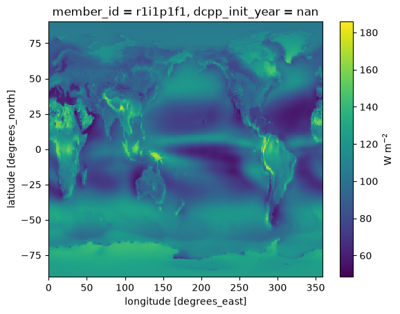
Positive values for rsut indicate a positive-up convention. For SW we want to compute:
where the “Down” terms cancel because clouds have no effect on insolation.
ctrl_SWCRE = -ctrl_state.rsut + ctrl_state.rsutcs
pert_SWCRE = -pert_state.rsut + pert_state.rsutcs
dSWCRE = pert_SWCRE - ctrl_SWCRECheck the CRE to make sure the sign is correct:
ctrl_SWCRE.mean(dim='month').plot(cbar_kwargs={'label': 'W m$^{-2}$'})Could not determine bucket type for bucket name cmip6: Your default credentials were not found. To set up Application Default Credentials, see https://cloud.google.com/docs/authentication/external/set-up-adc for more information., falling back to GCSFileSystem
Could not determine bucket type for bucket name cmip6: Your default credentials were not found. To set up Application Default Credentials, see https://cloud.google.com/docs/authentication/external/set-up-adc for more information., falling back to GCSFileSystem
Could not determine bucket type for bucket name cmip6: Your default credentials were not found. To set up Application Default Credentials, see https://cloud.google.com/docs/authentication/external/set-up-adc for more information., falling back to GCSFileSystem
Could not determine bucket type for bucket name cmip6: Your default credentials were not found. To set up Application Default Credentials, see https://cloud.google.com/docs/authentication/external/set-up-adc for more information., falling back to GCSFileSystem
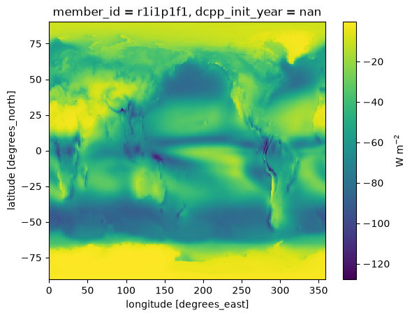
As expected, negative values indicate that on the SW side, clouds have a cooling effect. Here is the change in SW CRE:
dSWCRE.mean(dim='month').plot(cbar_kwargs={'label': 'W m$^{-2}$'})Could not determine bucket type for bucket name cmip6: Your default credentials were not found. To set up Application Default Credentials, see https://cloud.google.com/docs/authentication/external/set-up-adc for more information., falling back to GCSFileSystem
Could not determine bucket type for bucket name cmip6: Your default credentials were not found. To set up Application Default Credentials, see https://cloud.google.com/docs/authentication/external/set-up-adc for more information., falling back to GCSFileSystem
Could not determine bucket type for bucket name cmip6: Your default credentials were not found. To set up Application Default Credentials, see https://cloud.google.com/docs/authentication/external/set-up-adc for more information., falling back to GCSFileSystem
Could not determine bucket type for bucket name cmip6: Your default credentials were not found. To set up Application Default Credentials, see https://cloud.google.com/docs/authentication/external/set-up-adc for more information., falling back to GCSFileSystem
Could not determine bucket type for bucket name cmip6: Your default credentials were not found. To set up Application Default Credentials, see https://cloud.google.com/docs/authentication/external/set-up-adc for more information., falling back to GCSFileSystem
Could not determine bucket type for bucket name cmip6: Your default credentials were not found. To set up Application Default Credentials, see https://cloud.google.com/docs/authentication/external/set-up-adc for more information., falling back to GCSFileSystem
Could not determine bucket type for bucket name cmip6: Your default credentials were not found. To set up Application Default Credentials, see https://cloud.google.com/docs/authentication/external/set-up-adc for more information., falling back to GCSFileSystem
Could not determine bucket type for bucket name cmip6: Your default credentials were not found. To set up Application Default Credentials, see https://cloud.google.com/docs/authentication/external/set-up-adc for more information., falling back to GCSFileSystem
Could not determine bucket type for bucket name cmip6: Your default credentials were not found. To set up Application Default Credentials, see https://cloud.google.com/docs/authentication/external/set-up-adc for more information., falling back to GCSFileSystem
Could not determine bucket type for bucket name cmip6: Your default credentials were not found. To set up Application Default Credentials, see https://cloud.google.com/docs/authentication/external/set-up-adc for more information., falling back to GCSFileSystem
Could not determine bucket type for bucket name cmip6: Your default credentials were not found. To set up Application Default Credentials, see https://cloud.google.com/docs/authentication/external/set-up-adc for more information., falling back to GCSFileSystem
Could not determine bucket type for bucket name cmip6: Your default credentials were not found. To set up Application Default Credentials, see https://cloud.google.com/docs/authentication/external/set-up-adc for more information., falling back to GCSFileSystem
Could not determine bucket type for bucket name cmip6: Your default credentials were not found. To set up Application Default Credentials, see https://cloud.google.com/docs/authentication/external/set-up-adc for more information., falling back to GCSFileSystem
Could not determine bucket type for bucket name cmip6: Your default credentials were not found. To set up Application Default Credentials, see https://cloud.google.com/docs/authentication/external/set-up-adc for more information., falling back to GCSFileSystem
Could not determine bucket type for bucket name cmip6: Your default credentials were not found. To set up Application Default Credentials, see https://cloud.google.com/docs/authentication/external/set-up-adc for more information., falling back to GCSFileSystem
Could not determine bucket type for bucket name cmip6: Your default credentials were not found. To set up Application Default Credentials, see https://cloud.google.com/docs/authentication/external/set-up-adc for more information., falling back to GCSFileSystem
Could not determine bucket type for bucket name cmip6: Your default credentials were not found. To set up Application Default Credentials, see https://cloud.google.com/docs/authentication/external/set-up-adc for more information., falling back to GCSFileSystem
Could not determine bucket type for bucket name cmip6: Your default credentials were not found. To set up Application Default Credentials, see https://cloud.google.com/docs/authentication/external/set-up-adc for more information., falling back to GCSFileSystem
Could not determine bucket type for bucket name cmip6: Your default credentials were not found. To set up Application Default Credentials, see https://cloud.google.com/docs/authentication/external/set-up-adc for more information., falling back to GCSFileSystem
Could not determine bucket type for bucket name cmip6: Your default credentials were not found. To set up Application Default Credentials, see https://cloud.google.com/docs/authentication/external/set-up-adc for more information., falling back to GCSFileSystem
Could not determine bucket type for bucket name cmip6: Your default credentials were not found. To set up Application Default Credentials, see https://cloud.google.com/docs/authentication/external/set-up-adc for more information., falling back to GCSFileSystem
Could not determine bucket type for bucket name cmip6: Your default credentials were not found. To set up Application Default Credentials, see https://cloud.google.com/docs/authentication/external/set-up-adc for more information., falling back to GCSFileSystem
Could not determine bucket type for bucket name cmip6: Your default credentials were not found. To set up Application Default Credentials, see https://cloud.google.com/docs/authentication/external/set-up-adc for more information., falling back to GCSFileSystem
Could not determine bucket type for bucket name cmip6: Your default credentials were not found. To set up Application Default Credentials, see https://cloud.google.com/docs/authentication/external/set-up-adc for more information., falling back to GCSFileSystem
Could not determine bucket type for bucket name cmip6: Your default credentials were not found. To set up Application Default Credentials, see https://cloud.google.com/docs/authentication/external/set-up-adc for more information., falling back to GCSFileSystem
Could not determine bucket type for bucket name cmip6: Your default credentials were not found. To set up Application Default Credentials, see https://cloud.google.com/docs/authentication/external/set-up-adc for more information., falling back to GCSFileSystem
Could not determine bucket type for bucket name cmip6: Your default credentials were not found. To set up Application Default Credentials, see https://cloud.google.com/docs/authentication/external/set-up-adc for more information., falling back to GCSFileSystem
Could not determine bucket type for bucket name cmip6: Your default credentials were not found. To set up Application Default Credentials, see https://cloud.google.com/docs/authentication/external/set-up-adc for more information., falling back to GCSFileSystem
Could not determine bucket type for bucket name cmip6: Your default credentials were not found. To set up Application Default Credentials, see https://cloud.google.com/docs/authentication/external/set-up-adc for more information., falling back to GCSFileSystem
Could not determine bucket type for bucket name cmip6: Your default credentials were not found. To set up Application Default Credentials, see https://cloud.google.com/docs/authentication/external/set-up-adc for more information., falling back to GCSFileSystem
Could not determine bucket type for bucket name cmip6: Your default credentials were not found. To set up Application Default Credentials, see https://cloud.google.com/docs/authentication/external/set-up-adc for more information., falling back to GCSFileSystem
Could not determine bucket type for bucket name cmip6: Your default credentials were not found. To set up Application Default Credentials, see https://cloud.google.com/docs/authentication/external/set-up-adc for more information., falling back to GCSFileSystem
Could not determine bucket type for bucket name cmip6: Your default credentials were not found. To set up Application Default Credentials, see https://cloud.google.com/docs/authentication/external/set-up-adc for more information., falling back to GCSFileSystem
Could not determine bucket type for bucket name cmip6: Your default credentials were not found. To set up Application Default Credentials, see https://cloud.google.com/docs/authentication/external/set-up-adc for more information., falling back to GCSFileSystem
Could not determine bucket type for bucket name cmip6: Your default credentials were not found. To set up Application Default Credentials, see https://cloud.google.com/docs/authentication/external/set-up-adc for more information., falling back to GCSFileSystem
Could not determine bucket type for bucket name cmip6: Your default credentials were not found. To set up Application Default Credentials, see https://cloud.google.com/docs/authentication/external/set-up-adc for more information., falling back to GCSFileSystem
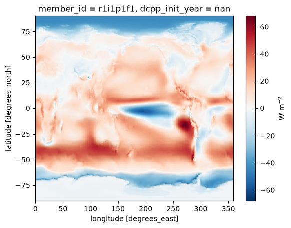
There is reduced (low) cloud cover under the CO2 forcing, so we can interpret this as clouds cooling the planet less under CO2 forcing, implying a positive feedback. Next, the LW version, where we use TOA outgoing longwave radiation:
ctrl_state.rlut.mean(dim='month').plot(cbar_kwargs={'label': 'W m$^{-2}$'})Could not determine bucket type for bucket name cmip6: Your default credentials were not found. To set up Application Default Credentials, see https://cloud.google.com/docs/authentication/external/set-up-adc for more information., falling back to GCSFileSystem
Could not determine bucket type for bucket name cmip6: Your default credentials were not found. To set up Application Default Credentials, see https://cloud.google.com/docs/authentication/external/set-up-adc for more information., falling back to GCSFileSystem
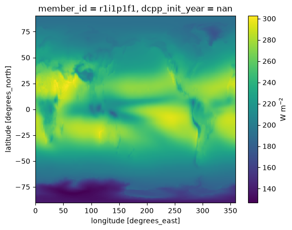
Positive-up is also used for rlut, so the calculation is similar:
where the “Down” terms here are just zero.
ctrl_LWCRE = -(ctrl_state.rlut - ctrl_state.rlutcs)
pert_LWCRE = -(pert_state.rlut - pert_state.rlutcs)
dLWCRE = pert_LWCRE - ctrl_LWCREctrl_LWCRE.mean(dim='month').plot(cbar_kwargs={'label': 'W m$^{-2}$'})Could not determine bucket type for bucket name cmip6: Your default credentials were not found. To set up Application Default Credentials, see https://cloud.google.com/docs/authentication/external/set-up-adc for more information., falling back to GCSFileSystem
Could not determine bucket type for bucket name cmip6: Your default credentials were not found. To set up Application Default Credentials, see https://cloud.google.com/docs/authentication/external/set-up-adc for more information., falling back to GCSFileSystem
Could not determine bucket type for bucket name cmip6: Your default credentials were not found. To set up Application Default Credentials, see https://cloud.google.com/docs/authentication/external/set-up-adc for more information., falling back to GCSFileSystem
Could not determine bucket type for bucket name cmip6: Your default credentials were not found. To set up Application Default Credentials, see https://cloud.google.com/docs/authentication/external/set-up-adc for more information., falling back to GCSFileSystem
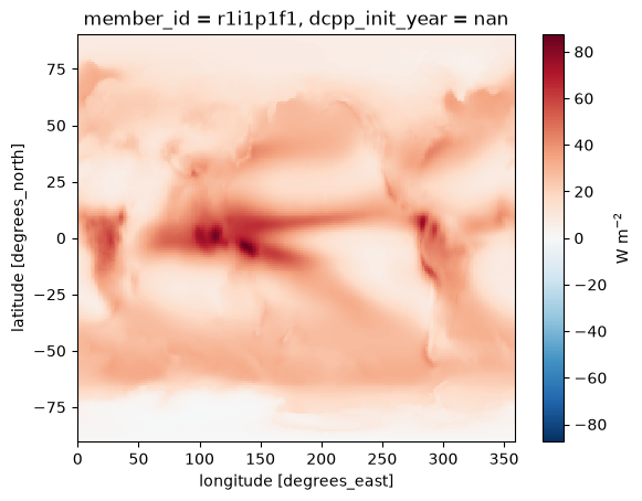
On the LW side, clouds have a warming effect. Here is the change in LW CRE under the CO2 forcing:
dLWCRE.mean(dim='month').plot(cbar_kwargs={'label': 'W m$^{-2}$'})Could not determine bucket type for bucket name cmip6: Your default credentials were not found. To set up Application Default Credentials, see https://cloud.google.com/docs/authentication/external/set-up-adc for more information., falling back to GCSFileSystem
Could not determine bucket type for bucket name cmip6: Your default credentials were not found. To set up Application Default Credentials, see https://cloud.google.com/docs/authentication/external/set-up-adc for more information., falling back to GCSFileSystem
Could not determine bucket type for bucket name cmip6: Your default credentials were not found. To set up Application Default Credentials, see https://cloud.google.com/docs/authentication/external/set-up-adc for more information., falling back to GCSFileSystem
Could not determine bucket type for bucket name cmip6: Your default credentials were not found. To set up Application Default Credentials, see https://cloud.google.com/docs/authentication/external/set-up-adc for more information., falling back to GCSFileSystem
Could not determine bucket type for bucket name cmip6: Your default credentials were not found. To set up Application Default Credentials, see https://cloud.google.com/docs/authentication/external/set-up-adc for more information., falling back to GCSFileSystem
Could not determine bucket type for bucket name cmip6: Your default credentials were not found. To set up Application Default Credentials, see https://cloud.google.com/docs/authentication/external/set-up-adc for more information., falling back to GCSFileSystem
Could not determine bucket type for bucket name cmip6: Your default credentials were not found. To set up Application Default Credentials, see https://cloud.google.com/docs/authentication/external/set-up-adc for more information., falling back to GCSFileSystem
Could not determine bucket type for bucket name cmip6: Your default credentials were not found. To set up Application Default Credentials, see https://cloud.google.com/docs/authentication/external/set-up-adc for more information., falling back to GCSFileSystem
Could not determine bucket type for bucket name cmip6: Your default credentials were not found. To set up Application Default Credentials, see https://cloud.google.com/docs/authentication/external/set-up-adc for more information., falling back to GCSFileSystem
Could not determine bucket type for bucket name cmip6: Your default credentials were not found. To set up Application Default Credentials, see https://cloud.google.com/docs/authentication/external/set-up-adc for more information., falling back to GCSFileSystem
Could not determine bucket type for bucket name cmip6: Your default credentials were not found. To set up Application Default Credentials, see https://cloud.google.com/docs/authentication/external/set-up-adc for more information., falling back to GCSFileSystem
Could not determine bucket type for bucket name cmip6: Your default credentials were not found. To set up Application Default Credentials, see https://cloud.google.com/docs/authentication/external/set-up-adc for more information., falling back to GCSFileSystem
Could not determine bucket type for bucket name cmip6: Your default credentials were not found. To set up Application Default Credentials, see https://cloud.google.com/docs/authentication/external/set-up-adc for more information., falling back to GCSFileSystem
Could not determine bucket type for bucket name cmip6: Your default credentials were not found. To set up Application Default Credentials, see https://cloud.google.com/docs/authentication/external/set-up-adc for more information., falling back to GCSFileSystem
Could not determine bucket type for bucket name cmip6: Your default credentials were not found. To set up Application Default Credentials, see https://cloud.google.com/docs/authentication/external/set-up-adc for more information., falling back to GCSFileSystem
Could not determine bucket type for bucket name cmip6: Your default credentials were not found. To set up Application Default Credentials, see https://cloud.google.com/docs/authentication/external/set-up-adc for more information., falling back to GCSFileSystem
Could not determine bucket type for bucket name cmip6: Your default credentials were not found. To set up Application Default Credentials, see https://cloud.google.com/docs/authentication/external/set-up-adc for more information., falling back to GCSFileSystem
Could not determine bucket type for bucket name cmip6: Your default credentials were not found. To set up Application Default Credentials, see https://cloud.google.com/docs/authentication/external/set-up-adc for more information., falling back to GCSFileSystem
Could not determine bucket type for bucket name cmip6: Your default credentials were not found. To set up Application Default Credentials, see https://cloud.google.com/docs/authentication/external/set-up-adc for more information., falling back to GCSFileSystem
Could not determine bucket type for bucket name cmip6: Your default credentials were not found. To set up Application Default Credentials, see https://cloud.google.com/docs/authentication/external/set-up-adc for more information., falling back to GCSFileSystem
Could not determine bucket type for bucket name cmip6: Your default credentials were not found. To set up Application Default Credentials, see https://cloud.google.com/docs/authentication/external/set-up-adc for more information., falling back to GCSFileSystem
Could not determine bucket type for bucket name cmip6: Your default credentials were not found. To set up Application Default Credentials, see https://cloud.google.com/docs/authentication/external/set-up-adc for more information., falling back to GCSFileSystem
Could not determine bucket type for bucket name cmip6: Your default credentials were not found. To set up Application Default Credentials, see https://cloud.google.com/docs/authentication/external/set-up-adc for more information., falling back to GCSFileSystem
Could not determine bucket type for bucket name cmip6: Your default credentials were not found. To set up Application Default Credentials, see https://cloud.google.com/docs/authentication/external/set-up-adc for more information., falling back to GCSFileSystem
Could not determine bucket type for bucket name cmip6: Your default credentials were not found. To set up Application Default Credentials, see https://cloud.google.com/docs/authentication/external/set-up-adc for more information., falling back to GCSFileSystem
Could not determine bucket type for bucket name cmip6: Your default credentials were not found. To set up Application Default Credentials, see https://cloud.google.com/docs/authentication/external/set-up-adc for more information., falling back to GCSFileSystem
Could not determine bucket type for bucket name cmip6: Your default credentials were not found. To set up Application Default Credentials, see https://cloud.google.com/docs/authentication/external/set-up-adc for more information., falling back to GCSFileSystem
Could not determine bucket type for bucket name cmip6: Your default credentials were not found. To set up Application Default Credentials, see https://cloud.google.com/docs/authentication/external/set-up-adc for more information., falling back to GCSFileSystem
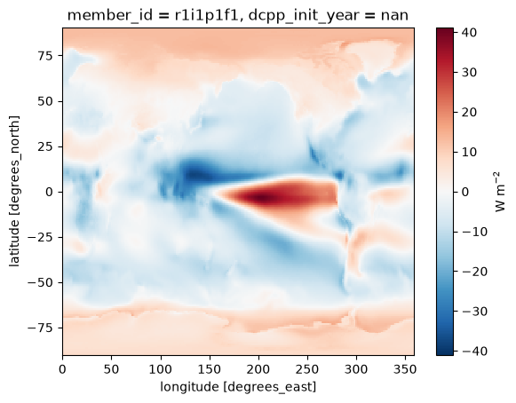
Adjusting CRE to get cloud feebacks
CRE partially masks some non-cloud feedbacks, so CRE needs to be adjusted to account for this.
Plots
def add_cyclic_point(xarray_obj, dim='lon', period=360):
if period is None:
period = xarray_obj.sizes[dim] / xarray_obj.coords[dim][:2].diff(dim).item()
first_point = xarray_obj.isel({dim: slice(1)})
first_point.coords[dim] = first_point.coords[dim]+period
return xr.concat([xarray_obj, first_point], dim=dim)ann_planck_feedback = planck_feedback.mean(dim='month').load()
ann_lapserate_feedback = lapserate_feedback.mean(dim='month').load()
ann_lwq_feedback = lwq_feedback.mean(dim='month').load()
ann_swq_feedback = swq_feedback.mean(dim='month').load()Could not determine bucket type for bucket name cmip6: Your default credentials were not found. To set up Application Default Credentials, see https://cloud.google.com/docs/authentication/external/set-up-adc for more information., falling back to GCSFileSystem
Could not determine bucket type for bucket name cmip6: Your default credentials were not found. To set up Application Default Credentials, see https://cloud.google.com/docs/authentication/external/set-up-adc for more information., falling back to GCSFileSystem
Could not determine bucket type for bucket name cmip6: Your default credentials were not found. To set up Application Default Credentials, see https://cloud.google.com/docs/authentication/external/set-up-adc for more information., falling back to GCSFileSystem
Could not determine bucket type for bucket name cmip6: Your default credentials were not found. To set up Application Default Credentials, see https://cloud.google.com/docs/authentication/external/set-up-adc for more information., falling back to GCSFileSystem
Could not determine bucket type for bucket name cmip6: Your default credentials were not found. To set up Application Default Credentials, see https://cloud.google.com/docs/authentication/external/set-up-adc for more information., falling back to GCSFileSystem
Could not determine bucket type for bucket name cmip6: Your default credentials were not found. To set up Application Default Credentials, see https://cloud.google.com/docs/authentication/external/set-up-adc for more information., falling back to GCSFileSystem
Could not determine bucket type for bucket name cmip6: Your default credentials were not found. To set up Application Default Credentials, see https://cloud.google.com/docs/authentication/external/set-up-adc for more information., falling back to GCSFileSystem
Could not determine bucket type for bucket name cmip6: Your default credentials were not found. To set up Application Default Credentials, see https://cloud.google.com/docs/authentication/external/set-up-adc for more information., falling back to GCSFileSystem
Could not determine bucket type for bucket name cmip6: Your default credentials were not found. To set up Application Default Credentials, see https://cloud.google.com/docs/authentication/external/set-up-adc for more information., falling back to GCSFileSystem
Could not determine bucket type for bucket name cmip6: Your default credentials were not found. To set up Application Default Credentials, see https://cloud.google.com/docs/authentication/external/set-up-adc for more information., falling back to GCSFileSystem
Could not determine bucket type for bucket name cmip6: Your default credentials were not found. To set up Application Default Credentials, see https://cloud.google.com/docs/authentication/external/set-up-adc for more information., falling back to GCSFileSystem
Could not determine bucket type for bucket name cmip6: Your default credentials were not found. To set up Application Default Credentials, see https://cloud.google.com/docs/authentication/external/set-up-adc for more information., falling back to GCSFileSystem
Could not determine bucket type for bucket name cmip6: Your default credentials were not found. To set up Application Default Credentials, see https://cloud.google.com/docs/authentication/external/set-up-adc for more information., falling back to GCSFileSystem
Could not determine bucket type for bucket name cmip6: Your default credentials were not found. To set up Application Default Credentials, see https://cloud.google.com/docs/authentication/external/set-up-adc for more information., falling back to GCSFileSystem
Could not determine bucket type for bucket name cmip6: Your default credentials were not found. To set up Application Default Credentials, see https://cloud.google.com/docs/authentication/external/set-up-adc for more information., falling back to GCSFileSystem
Could not determine bucket type for bucket name cmip6: Your default credentials were not found. To set up Application Default Credentials, see https://cloud.google.com/docs/authentication/external/set-up-adc for more information., falling back to GCSFileSystem
Could not determine bucket type for bucket name cmip6: Your default credentials were not found. To set up Application Default Credentials, see https://cloud.google.com/docs/authentication/external/set-up-adc for more information., falling back to GCSFileSystem
Could not determine bucket type for bucket name cmip6: Your default credentials were not found. To set up Application Default Credentials, see https://cloud.google.com/docs/authentication/external/set-up-adc for more information., falling back to GCSFileSystem
Could not determine bucket type for bucket name cmip6: Your default credentials were not found. To set up Application Default Credentials, see https://cloud.google.com/docs/authentication/external/set-up-adc for more information., falling back to GCSFileSystem
Could not determine bucket type for bucket name cmip6: Your default credentials were not found. To set up Application Default Credentials, see https://cloud.google.com/docs/authentication/external/set-up-adc for more information., falling back to GCSFileSystem
Could not determine bucket type for bucket name cmip6: Your default credentials were not found. To set up Application Default Credentials, see https://cloud.google.com/docs/authentication/external/set-up-adc for more information., falling back to GCSFileSystem
Could not determine bucket type for bucket name cmip6: Your default credentials were not found. To set up Application Default Credentials, see https://cloud.google.com/docs/authentication/external/set-up-adc for more information., falling back to GCSFileSystem
Could not determine bucket type for bucket name cmip6: Your default credentials were not found. To set up Application Default Credentials, see https://cloud.google.com/docs/authentication/external/set-up-adc for more information., falling back to GCSFileSystem
Could not determine bucket type for bucket name cmip6: Your default credentials were not found. To set up Application Default Credentials, see https://cloud.google.com/docs/authentication/external/set-up-adc for more information., falling back to GCSFileSystem
Could not determine bucket type for bucket name cmip6: Your default credentials were not found. To set up Application Default Credentials, see https://cloud.google.com/docs/authentication/external/set-up-adc for more information., falling back to GCSFileSystem
Could not determine bucket type for bucket name cmip6: Your default credentials were not found. To set up Application Default Credentials, see https://cloud.google.com/docs/authentication/external/set-up-adc for more information., falling back to GCSFileSystem
Could not determine bucket type for bucket name cmip6: Your default credentials were not found. To set up Application Default Credentials, see https://cloud.google.com/docs/authentication/external/set-up-adc for more information., falling back to GCSFileSystem
Could not determine bucket type for bucket name cmip6: Your default credentials were not found. To set up Application Default Credentials, see https://cloud.google.com/docs/authentication/external/set-up-adc for more information., falling back to GCSFileSystem
Could not determine bucket type for bucket name cmip6: Your default credentials were not found. To set up Application Default Credentials, see https://cloud.google.com/docs/authentication/external/set-up-adc for more information., falling back to GCSFileSystem
Could not determine bucket type for bucket name cmip6: Your default credentials were not found. To set up Application Default Credentials, see https://cloud.google.com/docs/authentication/external/set-up-adc for more information., falling back to GCSFileSystem
Could not determine bucket type for bucket name cmip6: Your default credentials were not found. To set up Application Default Credentials, see https://cloud.google.com/docs/authentication/external/set-up-adc for more information., falling back to GCSFileSystem
Could not determine bucket type for bucket name cmip6: Your default credentials were not found. To set up Application Default Credentials, see https://cloud.google.com/docs/authentication/external/set-up-adc for more information., falling back to GCSFileSystem
Could not determine bucket type for bucket name cmip6: Your default credentials were not found. To set up Application Default Credentials, see https://cloud.google.com/docs/authentication/external/set-up-adc for more information., falling back to GCSFileSystem
Could not determine bucket type for bucket name cmip6: Your default credentials were not found. To set up Application Default Credentials, see https://cloud.google.com/docs/authentication/external/set-up-adc for more information., falling back to GCSFileSystem
Could not determine bucket type for bucket name cmip6: Your default credentials were not found. To set up Application Default Credentials, see https://cloud.google.com/docs/authentication/external/set-up-adc for more information., falling back to GCSFileSystem
Could not determine bucket type for bucket name cmip6: Your default credentials were not found. To set up Application Default Credentials, see https://cloud.google.com/docs/authentication/external/set-up-adc for more information., falling back to GCSFileSystem
Could not determine bucket type for bucket name cmip6: Your default credentials were not found. To set up Application Default Credentials, see https://cloud.google.com/docs/authentication/external/set-up-adc for more information., falling back to GCSFileSystem
Could not determine bucket type for bucket name cmip6: Your default credentials were not found. To set up Application Default Credentials, see https://cloud.google.com/docs/authentication/external/set-up-adc for more information., falling back to GCSFileSystem
Could not determine bucket type for bucket name cmip6: Your default credentials were not found. To set up Application Default Credentials, see https://cloud.google.com/docs/authentication/external/set-up-adc for more information., falling back to GCSFileSystem
Could not determine bucket type for bucket name cmip6: Your default credentials were not found. To set up Application Default Credentials, see https://cloud.google.com/docs/authentication/external/set-up-adc for more information., falling back to GCSFileSystem
Could not determine bucket type for bucket name cmip6: Your default credentials were not found. To set up Application Default Credentials, see https://cloud.google.com/docs/authentication/external/set-up-adc for more information., falling back to GCSFileSystem
Could not determine bucket type for bucket name cmip6: Your default credentials were not found. To set up Application Default Credentials, see https://cloud.google.com/docs/authentication/external/set-up-adc for more information., falling back to GCSFileSystem
Could not determine bucket type for bucket name cmip6: Your default credentials were not found. To set up Application Default Credentials, see https://cloud.google.com/docs/authentication/external/set-up-adc for more information., falling back to GCSFileSystem
Could not determine bucket type for bucket name cmip6: Your default credentials were not found. To set up Application Default Credentials, see https://cloud.google.com/docs/authentication/external/set-up-adc for more information., falling back to GCSFileSystem
Could not determine bucket type for bucket name cmip6: Your default credentials were not found. To set up Application Default Credentials, see https://cloud.google.com/docs/authentication/external/set-up-adc for more information., falling back to GCSFileSystem
Could not determine bucket type for bucket name cmip6: Your default credentials were not found. To set up Application Default Credentials, see https://cloud.google.com/docs/authentication/external/set-up-adc for more information., falling back to GCSFileSystem
Could not determine bucket type for bucket name cmip6: Your default credentials were not found. To set up Application Default Credentials, see https://cloud.google.com/docs/authentication/external/set-up-adc for more information., falling back to GCSFileSystem
Could not determine bucket type for bucket name cmip6: Your default credentials were not found. To set up Application Default Credentials, see https://cloud.google.com/docs/authentication/external/set-up-adc for more information., falling back to GCSFileSystem
Could not determine bucket type for bucket name cmip6: Your default credentials were not found. To set up Application Default Credentials, see https://cloud.google.com/docs/authentication/external/set-up-adc for more information., falling back to GCSFileSystem
Could not determine bucket type for bucket name cmip6: Your default credentials were not found. To set up Application Default Credentials, see https://cloud.google.com/docs/authentication/external/set-up-adc for more information., falling back to GCSFileSystem
Could not determine bucket type for bucket name cmip6: Your default credentials were not found. To set up Application Default Credentials, see https://cloud.google.com/docs/authentication/external/set-up-adc for more information., falling back to GCSFileSystem
Could not determine bucket type for bucket name cmip6: Your default credentials were not found. To set up Application Default Credentials, see https://cloud.google.com/docs/authentication/external/set-up-adc for more information., falling back to GCSFileSystem
Could not determine bucket type for bucket name cmip6: Your default credentials were not found. To set up Application Default Credentials, see https://cloud.google.com/docs/authentication/external/set-up-adc for more information., falling back to GCSFileSystem
Could not determine bucket type for bucket name cmip6: Your default credentials were not found. To set up Application Default Credentials, see https://cloud.google.com/docs/authentication/external/set-up-adc for more information., falling back to GCSFileSystem
Could not determine bucket type for bucket name cmip6: Your default credentials were not found. To set up Application Default Credentials, see https://cloud.google.com/docs/authentication/external/set-up-adc for more information., falling back to GCSFileSystem
Could not determine bucket type for bucket name cmip6: Your default credentials were not found. To set up Application Default Credentials, see https://cloud.google.com/docs/authentication/external/set-up-adc for more information., falling back to GCSFileSystem
Could not determine bucket type for bucket name cmip6: Your default credentials were not found. To set up Application Default Credentials, see https://cloud.google.com/docs/authentication/external/set-up-adc for more information., falling back to GCSFileSystem
Could not determine bucket type for bucket name cmip6: Your default credentials were not found. To set up Application Default Credentials, see https://cloud.google.com/docs/authentication/external/set-up-adc for more information., falling back to GCSFileSystem
Could not determine bucket type for bucket name cmip6: Your default credentials were not found. To set up Application Default Credentials, see https://cloud.google.com/docs/authentication/external/set-up-adc for more information., falling back to GCSFileSystem
Could not determine bucket type for bucket name cmip6: Your default credentials were not found. To set up Application Default Credentials, see https://cloud.google.com/docs/authentication/external/set-up-adc for more information., falling back to GCSFileSystem
Could not determine bucket type for bucket name cmip6: Your default credentials were not found. To set up Application Default Credentials, see https://cloud.google.com/docs/authentication/external/set-up-adc for more information., falling back to GCSFileSystem
Could not determine bucket type for bucket name cmip6: Your default credentials were not found. To set up Application Default Credentials, see https://cloud.google.com/docs/authentication/external/set-up-adc for more information., falling back to GCSFileSystem
Could not determine bucket type for bucket name cmip6: Your default credentials were not found. To set up Application Default Credentials, see https://cloud.google.com/docs/authentication/external/set-up-adc for more information., falling back to GCSFileSystem
Could not determine bucket type for bucket name cmip6: Your default credentials were not found. To set up Application Default Credentials, see https://cloud.google.com/docs/authentication/external/set-up-adc for more information., falling back to GCSFileSystem
Could not determine bucket type for bucket name cmip6: Your default credentials were not found. To set up Application Default Credentials, see https://cloud.google.com/docs/authentication/external/set-up-adc for more information., falling back to GCSFileSystem
Could not determine bucket type for bucket name cmip6: Your default credentials were not found. To set up Application Default Credentials, see https://cloud.google.com/docs/authentication/external/set-up-adc for more information., falling back to GCSFileSystem
Could not determine bucket type for bucket name cmip6: Your default credentials were not found. To set up Application Default Credentials, see https://cloud.google.com/docs/authentication/external/set-up-adc for more information., falling back to GCSFileSystem
Could not determine bucket type for bucket name cmip6: Your default credentials were not found. To set up Application Default Credentials, see https://cloud.google.com/docs/authentication/external/set-up-adc for more information., falling back to GCSFileSystem
Could not determine bucket type for bucket name cmip6: Your default credentials were not found. To set up Application Default Credentials, see https://cloud.google.com/docs/authentication/external/set-up-adc for more information., falling back to GCSFileSystem
Could not determine bucket type for bucket name cmip6: Your default credentials were not found. To set up Application Default Credentials, see https://cloud.google.com/docs/authentication/external/set-up-adc for more information., falling back to GCSFileSystem
Could not determine bucket type for bucket name cmip6: Your default credentials were not found. To set up Application Default Credentials, see https://cloud.google.com/docs/authentication/external/set-up-adc for more information., falling back to GCSFileSystem
Could not determine bucket type for bucket name cmip6: Your default credentials were not found. To set up Application Default Credentials, see https://cloud.google.com/docs/authentication/external/set-up-adc for more information., falling back to GCSFileSystem
Could not determine bucket type for bucket name cmip6: Your default credentials were not found. To set up Application Default Credentials, see https://cloud.google.com/docs/authentication/external/set-up-adc for more information., falling back to GCSFileSystem
Could not determine bucket type for bucket name cmip6: Your default credentials were not found. To set up Application Default Credentials, see https://cloud.google.com/docs/authentication/external/set-up-adc for more information., falling back to GCSFileSystem
Could not determine bucket type for bucket name cmip6: Your default credentials were not found. To set up Application Default Credentials, see https://cloud.google.com/docs/authentication/external/set-up-adc for more information., falling back to GCSFileSystem
Could not determine bucket type for bucket name cmip6: Your default credentials were not found. To set up Application Default Credentials, see https://cloud.google.com/docs/authentication/external/set-up-adc for more information., falling back to GCSFileSystem
Could not determine bucket type for bucket name cmip6: Your default credentials were not found. To set up Application Default Credentials, see https://cloud.google.com/docs/authentication/external/set-up-adc for more information., falling back to GCSFileSystem
Could not determine bucket type for bucket name cmip6: Your default credentials were not found. To set up Application Default Credentials, see https://cloud.google.com/docs/authentication/external/set-up-adc for more information., falling back to GCSFileSystem
Could not determine bucket type for bucket name cmip6: Your default credentials were not found. To set up Application Default Credentials, see https://cloud.google.com/docs/authentication/external/set-up-adc for more information., falling back to GCSFileSystem
Could not determine bucket type for bucket name cmip6: Your default credentials were not found. To set up Application Default Credentials, see https://cloud.google.com/docs/authentication/external/set-up-adc for more information., falling back to GCSFileSystem
Could not determine bucket type for bucket name cmip6: Your default credentials were not found. To set up Application Default Credentials, see https://cloud.google.com/docs/authentication/external/set-up-adc for more information., falling back to GCSFileSystem
Could not determine bucket type for bucket name cmip6: Your default credentials were not found. To set up Application Default Credentials, see https://cloud.google.com/docs/authentication/external/set-up-adc for more information., falling back to GCSFileSystem
Could not determine bucket type for bucket name cmip6: Your default credentials were not found. To set up Application Default Credentials, see https://cloud.google.com/docs/authentication/external/set-up-adc for more information., falling back to GCSFileSystem
Could not determine bucket type for bucket name cmip6: Your default credentials were not found. To set up Application Default Credentials, see https://cloud.google.com/docs/authentication/external/set-up-adc for more information., falling back to GCSFileSystem
Could not determine bucket type for bucket name cmip6: Your default credentials were not found. To set up Application Default Credentials, see https://cloud.google.com/docs/authentication/external/set-up-adc for more information., falling back to GCSFileSystem
Could not determine bucket type for bucket name cmip6: Your default credentials were not found. To set up Application Default Credentials, see https://cloud.google.com/docs/authentication/external/set-up-adc for more information., falling back to GCSFileSystem
Could not determine bucket type for bucket name cmip6: Your default credentials were not found. To set up Application Default Credentials, see https://cloud.google.com/docs/authentication/external/set-up-adc for more information., falling back to GCSFileSystem
Could not determine bucket type for bucket name cmip6: Your default credentials were not found. To set up Application Default Credentials, see https://cloud.google.com/docs/authentication/external/set-up-adc for more information., falling back to GCSFileSystem
Could not determine bucket type for bucket name cmip6: Your default credentials were not found. To set up Application Default Credentials, see https://cloud.google.com/docs/authentication/external/set-up-adc for more information., falling back to GCSFileSystem
Could not determine bucket type for bucket name cmip6: Your default credentials were not found. To set up Application Default Credentials, see https://cloud.google.com/docs/authentication/external/set-up-adc for more information., falling back to GCSFileSystem
Could not determine bucket type for bucket name cmip6: Your default credentials were not found. To set up Application Default Credentials, see https://cloud.google.com/docs/authentication/external/set-up-adc for more information., falling back to GCSFileSystem
Could not determine bucket type for bucket name cmip6: Your default credentials were not found. To set up Application Default Credentials, see https://cloud.google.com/docs/authentication/external/set-up-adc for more information., falling back to GCSFileSystem
Could not determine bucket type for bucket name cmip6: Your default credentials were not found. To set up Application Default Credentials, see https://cloud.google.com/docs/authentication/external/set-up-adc for more information., falling back to GCSFileSystem
Could not determine bucket type for bucket name cmip6: Your default credentials were not found. To set up Application Default Credentials, see https://cloud.google.com/docs/authentication/external/set-up-adc for more information., falling back to GCSFileSystem
Could not determine bucket type for bucket name cmip6: Your default credentials were not found. To set up Application Default Credentials, see https://cloud.google.com/docs/authentication/external/set-up-adc for more information., falling back to GCSFileSystem
Could not determine bucket type for bucket name cmip6: Your default credentials were not found. To set up Application Default Credentials, see https://cloud.google.com/docs/authentication/external/set-up-adc for more information., falling back to GCSFileSystem
Could not determine bucket type for bucket name cmip6: Your default credentials were not found. To set up Application Default Credentials, see https://cloud.google.com/docs/authentication/external/set-up-adc for more information., falling back to GCSFileSystem
Could not determine bucket type for bucket name cmip6: Your default credentials were not found. To set up Application Default Credentials, see https://cloud.google.com/docs/authentication/external/set-up-adc for more information., falling back to GCSFileSystem
Could not determine bucket type for bucket name cmip6: Your default credentials were not found. To set up Application Default Credentials, see https://cloud.google.com/docs/authentication/external/set-up-adc for more information., falling back to GCSFileSystem
Could not determine bucket type for bucket name cmip6: Your default credentials were not found. To set up Application Default Credentials, see https://cloud.google.com/docs/authentication/external/set-up-adc for more information., falling back to GCSFileSystem
Could not determine bucket type for bucket name cmip6: Your default credentials were not found. To set up Application Default Credentials, see https://cloud.google.com/docs/authentication/external/set-up-adc for more information., falling back to GCSFileSystem
Could not determine bucket type for bucket name cmip6: Your default credentials were not found. To set up Application Default Credentials, see https://cloud.google.com/docs/authentication/external/set-up-adc for more information., falling back to GCSFileSystem
Could not determine bucket type for bucket name cmip6: Your default credentials were not found. To set up Application Default Credentials, see https://cloud.google.com/docs/authentication/external/set-up-adc for more information., falling back to GCSFileSystem
Could not determine bucket type for bucket name cmip6: Your default credentials were not found. To set up Application Default Credentials, see https://cloud.google.com/docs/authentication/external/set-up-adc for more information., falling back to GCSFileSystem
Could not determine bucket type for bucket name cmip6: Your default credentials were not found. To set up Application Default Credentials, see https://cloud.google.com/docs/authentication/external/set-up-adc for more information., falling back to GCSFileSystem
Could not determine bucket type for bucket name cmip6: Your default credentials were not found. To set up Application Default Credentials, see https://cloud.google.com/docs/authentication/external/set-up-adc for more information., falling back to GCSFileSystem
Could not determine bucket type for bucket name cmip6: Your default credentials were not found. To set up Application Default Credentials, see https://cloud.google.com/docs/authentication/external/set-up-adc for more information., falling back to GCSFileSystem
Could not determine bucket type for bucket name cmip6: Your default credentials were not found. To set up Application Default Credentials, see https://cloud.google.com/docs/authentication/external/set-up-adc for more information., falling back to GCSFileSystem
Could not determine bucket type for bucket name cmip6: Your default credentials were not found. To set up Application Default Credentials, see https://cloud.google.com/docs/authentication/external/set-up-adc for more information., falling back to GCSFileSystem
Could not determine bucket type for bucket name cmip6: Your default credentials were not found. To set up Application Default Credentials, see https://cloud.google.com/docs/authentication/external/set-up-adc for more information., falling back to GCSFileSystem
Could not determine bucket type for bucket name cmip6: Your default credentials were not found. To set up Application Default Credentials, see https://cloud.google.com/docs/authentication/external/set-up-adc for more information., falling back to GCSFileSystem
Could not determine bucket type for bucket name cmip6: Your default credentials were not found. To set up Application Default Credentials, see https://cloud.google.com/docs/authentication/external/set-up-adc for more information., falling back to GCSFileSystem
Could not determine bucket type for bucket name cmip6: Your default credentials were not found. To set up Application Default Credentials, see https://cloud.google.com/docs/authentication/external/set-up-adc for more information., falling back to GCSFileSystem
Could not determine bucket type for bucket name cmip6: Your default credentials were not found. To set up Application Default Credentials, see https://cloud.google.com/docs/authentication/external/set-up-adc for more information., falling back to GCSFileSystem
Could not determine bucket type for bucket name cmip6: Your default credentials were not found. To set up Application Default Credentials, see https://cloud.google.com/docs/authentication/external/set-up-adc for more information., falling back to GCSFileSystem
Could not determine bucket type for bucket name cmip6: Your default credentials were not found. To set up Application Default Credentials, see https://cloud.google.com/docs/authentication/external/set-up-adc for more information., falling back to GCSFileSystem
Could not determine bucket type for bucket name cmip6: Your default credentials were not found. To set up Application Default Credentials, see https://cloud.google.com/docs/authentication/external/set-up-adc for more information., falling back to GCSFileSystem
Could not determine bucket type for bucket name cmip6: Your default credentials were not found. To set up Application Default Credentials, see https://cloud.google.com/docs/authentication/external/set-up-adc for more information., falling back to GCSFileSystem
Could not determine bucket type for bucket name cmip6: Your default credentials were not found. To set up Application Default Credentials, see https://cloud.google.com/docs/authentication/external/set-up-adc for more information., falling back to GCSFileSystem
Could not determine bucket type for bucket name cmip6: Your default credentials were not found. To set up Application Default Credentials, see https://cloud.google.com/docs/authentication/external/set-up-adc for more information., falling back to GCSFileSystem
Could not determine bucket type for bucket name cmip6: Your default credentials were not found. To set up Application Default Credentials, see https://cloud.google.com/docs/authentication/external/set-up-adc for more information., falling back to GCSFileSystem
Could not determine bucket type for bucket name cmip6: Your default credentials were not found. To set up Application Default Credentials, see https://cloud.google.com/docs/authentication/external/set-up-adc for more information., falling back to GCSFileSystem
Could not determine bucket type for bucket name cmip6: Your default credentials were not found. To set up Application Default Credentials, see https://cloud.google.com/docs/authentication/external/set-up-adc for more information., falling back to GCSFileSystem
Could not determine bucket type for bucket name cmip6: Your default credentials were not found. To set up Application Default Credentials, see https://cloud.google.com/docs/authentication/external/set-up-adc for more information., falling back to GCSFileSystem
Could not determine bucket type for bucket name cmip6: Your default credentials were not found. To set up Application Default Credentials, see https://cloud.google.com/docs/authentication/external/set-up-adc for more information., falling back to GCSFileSystem
Could not determine bucket type for bucket name cmip6: Your default credentials were not found. To set up Application Default Credentials, see https://cloud.google.com/docs/authentication/external/set-up-adc for more information., falling back to GCSFileSystem
Could not determine bucket type for bucket name cmip6: Your default credentials were not found. To set up Application Default Credentials, see https://cloud.google.com/docs/authentication/external/set-up-adc for more information., falling back to GCSFileSystem
Could not determine bucket type for bucket name cmip6: Your default credentials were not found. To set up Application Default Credentials, see https://cloud.google.com/docs/authentication/external/set-up-adc for more information., falling back to GCSFileSystem
Could not determine bucket type for bucket name cmip6: Your default credentials were not found. To set up Application Default Credentials, see https://cloud.google.com/docs/authentication/external/set-up-adc for more information., falling back to GCSFileSystem
Could not determine bucket type for bucket name cmip6: Your default credentials were not found. To set up Application Default Credentials, see https://cloud.google.com/docs/authentication/external/set-up-adc for more information., falling back to GCSFileSystem
Could not determine bucket type for bucket name cmip6: Your default credentials were not found. To set up Application Default Credentials, see https://cloud.google.com/docs/authentication/external/set-up-adc for more information., falling back to GCSFileSystem
Could not determine bucket type for bucket name cmip6: Your default credentials were not found. To set up Application Default Credentials, see https://cloud.google.com/docs/authentication/external/set-up-adc for more information., falling back to GCSFileSystem
Could not determine bucket type for bucket name cmip6: Your default credentials were not found. To set up Application Default Credentials, see https://cloud.google.com/docs/authentication/external/set-up-adc for more information., falling back to GCSFileSystem
Could not determine bucket type for bucket name cmip6: Your default credentials were not found. To set up Application Default Credentials, see https://cloud.google.com/docs/authentication/external/set-up-adc for more information., falling back to GCSFileSystem
Could not determine bucket type for bucket name cmip6: Your default credentials were not found. To set up Application Default Credentials, see https://cloud.google.com/docs/authentication/external/set-up-adc for more information., falling back to GCSFileSystem
Could not determine bucket type for bucket name cmip6: Your default credentials were not found. To set up Application Default Credentials, see https://cloud.google.com/docs/authentication/external/set-up-adc for more information., falling back to GCSFileSystem
Could not determine bucket type for bucket name cmip6: Your default credentials were not found. To set up Application Default Credentials, see https://cloud.google.com/docs/authentication/external/set-up-adc for more information., falling back to GCSFileSystem
Could not determine bucket type for bucket name cmip6: Your default credentials were not found. To set up Application Default Credentials, see https://cloud.google.com/docs/authentication/external/set-up-adc for more information., falling back to GCSFileSystem
Could not determine bucket type for bucket name cmip6: Your default credentials were not found. To set up Application Default Credentials, see https://cloud.google.com/docs/authentication/external/set-up-adc for more information., falling back to GCSFileSystem
Could not determine bucket type for bucket name cmip6: Your default credentials were not found. To set up Application Default Credentials, see https://cloud.google.com/docs/authentication/external/set-up-adc for more information., falling back to GCSFileSystem
Could not determine bucket type for bucket name cmip6: Your default credentials were not found. To set up Application Default Credentials, see https://cloud.google.com/docs/authentication/external/set-up-adc for more information., falling back to GCSFileSystem
Could not determine bucket type for bucket name cmip6: Your default credentials were not found. To set up Application Default Credentials, see https://cloud.google.com/docs/authentication/external/set-up-adc for more information., falling back to GCSFileSystem
Could not determine bucket type for bucket name cmip6: Your default credentials were not found. To set up Application Default Credentials, see https://cloud.google.com/docs/authentication/external/set-up-adc for more information., falling back to GCSFileSystem
Could not determine bucket type for bucket name cmip6: Your default credentials were not found. To set up Application Default Credentials, see https://cloud.google.com/docs/authentication/external/set-up-adc for more information., falling back to GCSFileSystem
Could not determine bucket type for bucket name cmip6: Your default credentials were not found. To set up Application Default Credentials, see https://cloud.google.com/docs/authentication/external/set-up-adc for more information., falling back to GCSFileSystem
Could not determine bucket type for bucket name cmip6: Your default credentials were not found. To set up Application Default Credentials, see https://cloud.google.com/docs/authentication/external/set-up-adc for more information., falling back to GCSFileSystem
Could not determine bucket type for bucket name cmip6: Your default credentials were not found. To set up Application Default Credentials, see https://cloud.google.com/docs/authentication/external/set-up-adc for more information., falling back to GCSFileSystem
Could not determine bucket type for bucket name cmip6: Your default credentials were not found. To set up Application Default Credentials, see https://cloud.google.com/docs/authentication/external/set-up-adc for more information., falling back to GCSFileSystem
Could not determine bucket type for bucket name cmip6: Your default credentials were not found. To set up Application Default Credentials, see https://cloud.google.com/docs/authentication/external/set-up-adc for more information., falling back to GCSFileSystem
Could not determine bucket type for bucket name cmip6: Your default credentials were not found. To set up Application Default Credentials, see https://cloud.google.com/docs/authentication/external/set-up-adc for more information., falling back to GCSFileSystem
Could not determine bucket type for bucket name cmip6: Your default credentials were not found. To set up Application Default Credentials, see https://cloud.google.com/docs/authentication/external/set-up-adc for more information., falling back to GCSFileSystem
Could not determine bucket type for bucket name cmip6: Your default credentials were not found. To set up Application Default Credentials, see https://cloud.google.com/docs/authentication/external/set-up-adc for more information., falling back to GCSFileSystem
Could not determine bucket type for bucket name cmip6: Your default credentials were not found. To set up Application Default Credentials, see https://cloud.google.com/docs/authentication/external/set-up-adc for more information., falling back to GCSFileSystem
Could not determine bucket type for bucket name cmip6: Your default credentials were not found. To set up Application Default Credentials, see https://cloud.google.com/docs/authentication/external/set-up-adc for more information., falling back to GCSFileSystem
Could not determine bucket type for bucket name cmip6: Your default credentials were not found. To set up Application Default Credentials, see https://cloud.google.com/docs/authentication/external/set-up-adc for more information., falling back to GCSFileSystem
Could not determine bucket type for bucket name cmip6: Your default credentials were not found. To set up Application Default Credentials, see https://cloud.google.com/docs/authentication/external/set-up-adc for more information., falling back to GCSFileSystem
Could not determine bucket type for bucket name cmip6: Your default credentials were not found. To set up Application Default Credentials, see https://cloud.google.com/docs/authentication/external/set-up-adc for more information., falling back to GCSFileSystem
Could not determine bucket type for bucket name cmip6: Your default credentials were not found. To set up Application Default Credentials, see https://cloud.google.com/docs/authentication/external/set-up-adc for more information., falling back to GCSFileSystem
Could not determine bucket type for bucket name cmip6: Your default credentials were not found. To set up Application Default Credentials, see https://cloud.google.com/docs/authentication/external/set-up-adc for more information., falling back to GCSFileSystem
Could not determine bucket type for bucket name cmip6: Your default credentials were not found. To set up Application Default Credentials, see https://cloud.google.com/docs/authentication/external/set-up-adc for more information., falling back to GCSFileSystem
Could not determine bucket type for bucket name cmip6: Your default credentials were not found. To set up Application Default Credentials, see https://cloud.google.com/docs/authentication/external/set-up-adc for more information., falling back to GCSFileSystem
Could not determine bucket type for bucket name cmip6: Your default credentials were not found. To set up Application Default Credentials, see https://cloud.google.com/docs/authentication/external/set-up-adc for more information., falling back to GCSFileSystem
Could not determine bucket type for bucket name cmip6: Your default credentials were not found. To set up Application Default Credentials, see https://cloud.google.com/docs/authentication/external/set-up-adc for more information., falling back to GCSFileSystem
Could not determine bucket type for bucket name cmip6: Your default credentials were not found. To set up Application Default Credentials, see https://cloud.google.com/docs/authentication/external/set-up-adc for more information., falling back to GCSFileSystem
Could not determine bucket type for bucket name cmip6: Your default credentials were not found. To set up Application Default Credentials, see https://cloud.google.com/docs/authentication/external/set-up-adc for more information., falling back to GCSFileSystem
Could not determine bucket type for bucket name cmip6: Your default credentials were not found. To set up Application Default Credentials, see https://cloud.google.com/docs/authentication/external/set-up-adc for more information., falling back to GCSFileSystem
Could not determine bucket type for bucket name cmip6: Your default credentials were not found. To set up Application Default Credentials, see https://cloud.google.com/docs/authentication/external/set-up-adc for more information., falling back to GCSFileSystem
Could not determine bucket type for bucket name cmip6: Your default credentials were not found. To set up Application Default Credentials, see https://cloud.google.com/docs/authentication/external/set-up-adc for more information., falling back to GCSFileSystem
Could not determine bucket type for bucket name cmip6: Your default credentials were not found. To set up Application Default Credentials, see https://cloud.google.com/docs/authentication/external/set-up-adc for more information., falling back to GCSFileSystem
Could not determine bucket type for bucket name cmip6: Your default credentials were not found. To set up Application Default Credentials, see https://cloud.google.com/docs/authentication/external/set-up-adc for more information., falling back to GCSFileSystem
Could not determine bucket type for bucket name cmip6: Your default credentials were not found. To set up Application Default Credentials, see https://cloud.google.com/docs/authentication/external/set-up-adc for more information., falling back to GCSFileSystem
Could not determine bucket type for bucket name cmip6: Your default credentials were not found. To set up Application Default Credentials, see https://cloud.google.com/docs/authentication/external/set-up-adc for more information., falling back to GCSFileSystem
Could not determine bucket type for bucket name cmip6: Your default credentials were not found. To set up Application Default Credentials, see https://cloud.google.com/docs/authentication/external/set-up-adc for more information., falling back to GCSFileSystem
Could not determine bucket type for bucket name cmip6: Your default credentials were not found. To set up Application Default Credentials, see https://cloud.google.com/docs/authentication/external/set-up-adc for more information., falling back to GCSFileSystem
Could not determine bucket type for bucket name cmip6: Your default credentials were not found. To set up Application Default Credentials, see https://cloud.google.com/docs/authentication/external/set-up-adc for more information., falling back to GCSFileSystem
Could not determine bucket type for bucket name cmip6: Your default credentials were not found. To set up Application Default Credentials, see https://cloud.google.com/docs/authentication/external/set-up-adc for more information., falling back to GCSFileSystem
Could not determine bucket type for bucket name cmip6: Your default credentials were not found. To set up Application Default Credentials, see https://cloud.google.com/docs/authentication/external/set-up-adc for more information., falling back to GCSFileSystem
Could not determine bucket type for bucket name cmip6: Your default credentials were not found. To set up Application Default Credentials, see https://cloud.google.com/docs/authentication/external/set-up-adc for more information., falling back to GCSFileSystem
Could not determine bucket type for bucket name cmip6: Your default credentials were not found. To set up Application Default Credentials, see https://cloud.google.com/docs/authentication/external/set-up-adc for more information., falling back to GCSFileSystem
Could not determine bucket type for bucket name cmip6: Your default credentials were not found. To set up Application Default Credentials, see https://cloud.google.com/docs/authentication/external/set-up-adc for more information., falling back to GCSFileSystem
Could not determine bucket type for bucket name cmip6: Your default credentials were not found. To set up Application Default Credentials, see https://cloud.google.com/docs/authentication/external/set-up-adc for more information., falling back to GCSFileSystem
Could not determine bucket type for bucket name cmip6: Your default credentials were not found. To set up Application Default Credentials, see https://cloud.google.com/docs/authentication/external/set-up-adc for more information., falling back to GCSFileSystem
Could not determine bucket type for bucket name cmip6: Your default credentials were not found. To set up Application Default Credentials, see https://cloud.google.com/docs/authentication/external/set-up-adc for more information., falling back to GCSFileSystem
Could not determine bucket type for bucket name cmip6: Your default credentials were not found. To set up Application Default Credentials, see https://cloud.google.com/docs/authentication/external/set-up-adc for more information., falling back to GCSFileSystem
Could not determine bucket type for bucket name cmip6: Your default credentials were not found. To set up Application Default Credentials, see https://cloud.google.com/docs/authentication/external/set-up-adc for more information., falling back to GCSFileSystem
Could not determine bucket type for bucket name cmip6: Your default credentials were not found. To set up Application Default Credentials, see https://cloud.google.com/docs/authentication/external/set-up-adc for more information., falling back to GCSFileSystem
Could not determine bucket type for bucket name cmip6: Your default credentials were not found. To set up Application Default Credentials, see https://cloud.google.com/docs/authentication/external/set-up-adc for more information., falling back to GCSFileSystem
Could not determine bucket type for bucket name cmip6: Your default credentials were not found. To set up Application Default Credentials, see https://cloud.google.com/docs/authentication/external/set-up-adc for more information., falling back to GCSFileSystem
Could not determine bucket type for bucket name cmip6: Your default credentials were not found. To set up Application Default Credentials, see https://cloud.google.com/docs/authentication/external/set-up-adc for more information., falling back to GCSFileSystem
Could not determine bucket type for bucket name cmip6: Your default credentials were not found. To set up Application Default Credentials, see https://cloud.google.com/docs/authentication/external/set-up-adc for more information., falling back to GCSFileSystem
Could not determine bucket type for bucket name cmip6: Your default credentials were not found. To set up Application Default Credentials, see https://cloud.google.com/docs/authentication/external/set-up-adc for more information., falling back to GCSFileSystem
Could not determine bucket type for bucket name cmip6: Your default credentials were not found. To set up Application Default Credentials, see https://cloud.google.com/docs/authentication/external/set-up-adc for more information., falling back to GCSFileSystem
Could not determine bucket type for bucket name cmip6: Your default credentials were not found. To set up Application Default Credentials, see https://cloud.google.com/docs/authentication/external/set-up-adc for more information., falling back to GCSFileSystem
Could not determine bucket type for bucket name cmip6: Your default credentials were not found. To set up Application Default Credentials, see https://cloud.google.com/docs/authentication/external/set-up-adc for more information., falling back to GCSFileSystem
Could not determine bucket type for bucket name cmip6: Your default credentials were not found. To set up Application Default Credentials, see https://cloud.google.com/docs/authentication/external/set-up-adc for more information., falling back to GCSFileSystem
Could not determine bucket type for bucket name cmip6: Your default credentials were not found. To set up Application Default Credentials, see https://cloud.google.com/docs/authentication/external/set-up-adc for more information., falling back to GCSFileSystem
Could not determine bucket type for bucket name cmip6: Your default credentials were not found. To set up Application Default Credentials, see https://cloud.google.com/docs/authentication/external/set-up-adc for more information., falling back to GCSFileSystem
Could not determine bucket type for bucket name cmip6: Your default credentials were not found. To set up Application Default Credentials, see https://cloud.google.com/docs/authentication/external/set-up-adc for more information., falling back to GCSFileSystem
Could not determine bucket type for bucket name cmip6: Your default credentials were not found. To set up Application Default Credentials, see https://cloud.google.com/docs/authentication/external/set-up-adc for more information., falling back to GCSFileSystem
Could not determine bucket type for bucket name cmip6: Your default credentials were not found. To set up Application Default Credentials, see https://cloud.google.com/docs/authentication/external/set-up-adc for more information., falling back to GCSFileSystem
Could not determine bucket type for bucket name cmip6: Your default credentials were not found. To set up Application Default Credentials, see https://cloud.google.com/docs/authentication/external/set-up-adc for more information., falling back to GCSFileSystem
Could not determine bucket type for bucket name cmip6: Your default credentials were not found. To set up Application Default Credentials, see https://cloud.google.com/docs/authentication/external/set-up-adc for more information., falling back to GCSFileSystem
Could not determine bucket type for bucket name cmip6: Your default credentials were not found. To set up Application Default Credentials, see https://cloud.google.com/docs/authentication/external/set-up-adc for more information., falling back to GCSFileSystem
Could not determine bucket type for bucket name cmip6: Your default credentials were not found. To set up Application Default Credentials, see https://cloud.google.com/docs/authentication/external/set-up-adc for more information., falling back to GCSFileSystem
Could not determine bucket type for bucket name cmip6: Your default credentials were not found. To set up Application Default Credentials, see https://cloud.google.com/docs/authentication/external/set-up-adc for more information., falling back to GCSFileSystem
Could not determine bucket type for bucket name cmip6: Your default credentials were not found. To set up Application Default Credentials, see https://cloud.google.com/docs/authentication/external/set-up-adc for more information., falling back to GCSFileSystem
Could not determine bucket type for bucket name cmip6: Your default credentials were not found. To set up Application Default Credentials, see https://cloud.google.com/docs/authentication/external/set-up-adc for more information., falling back to GCSFileSystem
Could not determine bucket type for bucket name cmip6: Your default credentials were not found. To set up Application Default Credentials, see https://cloud.google.com/docs/authentication/external/set-up-adc for more information., falling back to GCSFileSystem
Could not determine bucket type for bucket name cmip6: Your default credentials were not found. To set up Application Default Credentials, see https://cloud.google.com/docs/authentication/external/set-up-adc for more information., falling back to GCSFileSystem
Could not determine bucket type for bucket name cmip6: Your default credentials were not found. To set up Application Default Credentials, see https://cloud.google.com/docs/authentication/external/set-up-adc for more information., falling back to GCSFileSystem
Could not determine bucket type for bucket name cmip6: Your default credentials were not found. To set up Application Default Credentials, see https://cloud.google.com/docs/authentication/external/set-up-adc for more information., falling back to GCSFileSystem
Could not determine bucket type for bucket name cmip6: Your default credentials were not found. To set up Application Default Credentials, see https://cloud.google.com/docs/authentication/external/set-up-adc for more information., falling back to GCSFileSystem
Could not determine bucket type for bucket name cmip6: Your default credentials were not found. To set up Application Default Credentials, see https://cloud.google.com/docs/authentication/external/set-up-adc for more information., falling back to GCSFileSystem
Could not determine bucket type for bucket name cmip6: Your default credentials were not found. To set up Application Default Credentials, see https://cloud.google.com/docs/authentication/external/set-up-adc for more information., falling back to GCSFileSystem
Could not determine bucket type for bucket name cmip6: Your default credentials were not found. To set up Application Default Credentials, see https://cloud.google.com/docs/authentication/external/set-up-adc for more information., falling back to GCSFileSystem
Could not determine bucket type for bucket name cmip6: Your default credentials were not found. To set up Application Default Credentials, see https://cloud.google.com/docs/authentication/external/set-up-adc for more information., falling back to GCSFileSystem
Could not determine bucket type for bucket name cmip6: Your default credentials were not found. To set up Application Default Credentials, see https://cloud.google.com/docs/authentication/external/set-up-adc for more information., falling back to GCSFileSystem
Could not determine bucket type for bucket name cmip6: Your default credentials were not found. To set up Application Default Credentials, see https://cloud.google.com/docs/authentication/external/set-up-adc for more information., falling back to GCSFileSystem
Could not determine bucket type for bucket name cmip6: Your default credentials were not found. To set up Application Default Credentials, see https://cloud.google.com/docs/authentication/external/set-up-adc for more information., falling back to GCSFileSystem
Could not determine bucket type for bucket name cmip6: Your default credentials were not found. To set up Application Default Credentials, see https://cloud.google.com/docs/authentication/external/set-up-adc for more information., falling back to GCSFileSystem
Could not determine bucket type for bucket name cmip6: Your default credentials were not found. To set up Application Default Credentials, see https://cloud.google.com/docs/authentication/external/set-up-adc for more information., falling back to GCSFileSystem
Could not determine bucket type for bucket name cmip6: Your default credentials were not found. To set up Application Default Credentials, see https://cloud.google.com/docs/authentication/external/set-up-adc for more information., falling back to GCSFileSystem
Could not determine bucket type for bucket name cmip6: Your default credentials were not found. To set up Application Default Credentials, see https://cloud.google.com/docs/authentication/external/set-up-adc for more information., falling back to GCSFileSystem
Could not determine bucket type for bucket name cmip6: Your default credentials were not found. To set up Application Default Credentials, see https://cloud.google.com/docs/authentication/external/set-up-adc for more information., falling back to GCSFileSystem
Could not determine bucket type for bucket name cmip6: Your default credentials were not found. To set up Application Default Credentials, see https://cloud.google.com/docs/authentication/external/set-up-adc for more information., falling back to GCSFileSystem
Could not determine bucket type for bucket name cmip6: Your default credentials were not found. To set up Application Default Credentials, see https://cloud.google.com/docs/authentication/external/set-up-adc for more information., falling back to GCSFileSystem
Could not determine bucket type for bucket name cmip6: Your default credentials were not found. To set up Application Default Credentials, see https://cloud.google.com/docs/authentication/external/set-up-adc for more information., falling back to GCSFileSystem
Could not determine bucket type for bucket name cmip6: Your default credentials were not found. To set up Application Default Credentials, see https://cloud.google.com/docs/authentication/external/set-up-adc for more information., falling back to GCSFileSystem
Could not determine bucket type for bucket name cmip6: Your default credentials were not found. To set up Application Default Credentials, see https://cloud.google.com/docs/authentication/external/set-up-adc for more information., falling back to GCSFileSystem
Could not determine bucket type for bucket name cmip6: Your default credentials were not found. To set up Application Default Credentials, see https://cloud.google.com/docs/authentication/external/set-up-adc for more information., falling back to GCSFileSystem
Could not determine bucket type for bucket name cmip6: Your default credentials were not found. To set up Application Default Credentials, see https://cloud.google.com/docs/authentication/external/set-up-adc for more information., falling back to GCSFileSystem
Could not determine bucket type for bucket name cmip6: Your default credentials were not found. To set up Application Default Credentials, see https://cloud.google.com/docs/authentication/external/set-up-adc for more information., falling back to GCSFileSystem
Could not determine bucket type for bucket name cmip6: Your default credentials were not found. To set up Application Default Credentials, see https://cloud.google.com/docs/authentication/external/set-up-adc for more information., falling back to GCSFileSystem
Could not determine bucket type for bucket name cmip6: Your default credentials were not found. To set up Application Default Credentials, see https://cloud.google.com/docs/authentication/external/set-up-adc for more information., falling back to GCSFileSystem
Could not determine bucket type for bucket name cmip6: Your default credentials were not found. To set up Application Default Credentials, see https://cloud.google.com/docs/authentication/external/set-up-adc for more information., falling back to GCSFileSystem
Could not determine bucket type for bucket name cmip6: Your default credentials were not found. To set up Application Default Credentials, see https://cloud.google.com/docs/authentication/external/set-up-adc for more information., falling back to GCSFileSystem
Could not determine bucket type for bucket name cmip6: Your default credentials were not found. To set up Application Default Credentials, see https://cloud.google.com/docs/authentication/external/set-up-adc for more information., falling back to GCSFileSystem
Could not determine bucket type for bucket name cmip6: Your default credentials were not found. To set up Application Default Credentials, see https://cloud.google.com/docs/authentication/external/set-up-adc for more information., falling back to GCSFileSystem
Could not determine bucket type for bucket name cmip6: Your default credentials were not found. To set up Application Default Credentials, see https://cloud.google.com/docs/authentication/external/set-up-adc for more information., falling back to GCSFileSystem
Could not determine bucket type for bucket name cmip6: Your default credentials were not found. To set up Application Default Credentials, see https://cloud.google.com/docs/authentication/external/set-up-adc for more information., falling back to GCSFileSystem
Could not determine bucket type for bucket name cmip6: Your default credentials were not found. To set up Application Default Credentials, see https://cloud.google.com/docs/authentication/external/set-up-adc for more information., falling back to GCSFileSystem
Could not determine bucket type for bucket name cmip6: Your default credentials were not found. To set up Application Default Credentials, see https://cloud.google.com/docs/authentication/external/set-up-adc for more information., falling back to GCSFileSystem
Could not determine bucket type for bucket name cmip6: Your default credentials were not found. To set up Application Default Credentials, see https://cloud.google.com/docs/authentication/external/set-up-adc for more information., falling back to GCSFileSystem
Could not determine bucket type for bucket name cmip6: Your default credentials were not found. To set up Application Default Credentials, see https://cloud.google.com/docs/authentication/external/set-up-adc for more information., falling back to GCSFileSystem
Could not determine bucket type for bucket name cmip6: Your default credentials were not found. To set up Application Default Credentials, see https://cloud.google.com/docs/authentication/external/set-up-adc for more information., falling back to GCSFileSystem
Could not determine bucket type for bucket name cmip6: Your default credentials were not found. To set up Application Default Credentials, see https://cloud.google.com/docs/authentication/external/set-up-adc for more information., falling back to GCSFileSystem
Could not determine bucket type for bucket name cmip6: Your default credentials were not found. To set up Application Default Credentials, see https://cloud.google.com/docs/authentication/external/set-up-adc for more information., falling back to GCSFileSystem
Could not determine bucket type for bucket name cmip6: Your default credentials were not found. To set up Application Default Credentials, see https://cloud.google.com/docs/authentication/external/set-up-adc for more information., falling back to GCSFileSystem
Could not determine bucket type for bucket name cmip6: Your default credentials were not found. To set up Application Default Credentials, see https://cloud.google.com/docs/authentication/external/set-up-adc for more information., falling back to GCSFileSystem
Could not determine bucket type for bucket name cmip6: Your default credentials were not found. To set up Application Default Credentials, see https://cloud.google.com/docs/authentication/external/set-up-adc for more information., falling back to GCSFileSystem
Could not determine bucket type for bucket name cmip6: Your default credentials were not found. To set up Application Default Credentials, see https://cloud.google.com/docs/authentication/external/set-up-adc for more information., falling back to GCSFileSystem
Could not determine bucket type for bucket name cmip6: Your default credentials were not found. To set up Application Default Credentials, see https://cloud.google.com/docs/authentication/external/set-up-adc for more information., falling back to GCSFileSystem
Could not determine bucket type for bucket name cmip6: Your default credentials were not found. To set up Application Default Credentials, see https://cloud.google.com/docs/authentication/external/set-up-adc for more information., falling back to GCSFileSystem
Could not determine bucket type for bucket name cmip6: Your default credentials were not found. To set up Application Default Credentials, see https://cloud.google.com/docs/authentication/external/set-up-adc for more information., falling back to GCSFileSystem
Could not determine bucket type for bucket name cmip6: Your default credentials were not found. To set up Application Default Credentials, see https://cloud.google.com/docs/authentication/external/set-up-adc for more information., falling back to GCSFileSystem
Could not determine bucket type for bucket name cmip6: Your default credentials were not found. To set up Application Default Credentials, see https://cloud.google.com/docs/authentication/external/set-up-adc for more information., falling back to GCSFileSystem
Could not determine bucket type for bucket name cmip6: Your default credentials were not found. To set up Application Default Credentials, see https://cloud.google.com/docs/authentication/external/set-up-adc for more information., falling back to GCSFileSystem
Could not determine bucket type for bucket name cmip6: Your default credentials were not found. To set up Application Default Credentials, see https://cloud.google.com/docs/authentication/external/set-up-adc for more information., falling back to GCSFileSystem
Could not determine bucket type for bucket name cmip6: Your default credentials were not found. To set up Application Default Credentials, see https://cloud.google.com/docs/authentication/external/set-up-adc for more information., falling back to GCSFileSystem
Could not determine bucket type for bucket name cmip6: Your default credentials were not found. To set up Application Default Credentials, see https://cloud.google.com/docs/authentication/external/set-up-adc for more information., falling back to GCSFileSystem
Could not determine bucket type for bucket name cmip6: Your default credentials were not found. To set up Application Default Credentials, see https://cloud.google.com/docs/authentication/external/set-up-adc for more information., falling back to GCSFileSystem
Could not determine bucket type for bucket name cmip6: Your default credentials were not found. To set up Application Default Credentials, see https://cloud.google.com/docs/authentication/external/set-up-adc for more information., falling back to GCSFileSystem
Could not determine bucket type for bucket name cmip6: Your default credentials were not found. To set up Application Default Credentials, see https://cloud.google.com/docs/authentication/external/set-up-adc for more information., falling back to GCSFileSystem
Could not determine bucket type for bucket name cmip6: Your default credentials were not found. To set up Application Default Credentials, see https://cloud.google.com/docs/authentication/external/set-up-adc for more information., falling back to GCSFileSystem
Could not determine bucket type for bucket name cmip6: Your default credentials were not found. To set up Application Default Credentials, see https://cloud.google.com/docs/authentication/external/set-up-adc for more information., falling back to GCSFileSystem
Could not determine bucket type for bucket name cmip6: Your default credentials were not found. To set up Application Default Credentials, see https://cloud.google.com/docs/authentication/external/set-up-adc for more information., falling back to GCSFileSystem
Could not determine bucket type for bucket name cmip6: Your default credentials were not found. To set up Application Default Credentials, see https://cloud.google.com/docs/authentication/external/set-up-adc for more information., falling back to GCSFileSystem
Could not determine bucket type for bucket name cmip6: Your default credentials were not found. To set up Application Default Credentials, see https://cloud.google.com/docs/authentication/external/set-up-adc for more information., falling back to GCSFileSystem
Could not determine bucket type for bucket name cmip6: Your default credentials were not found. To set up Application Default Credentials, see https://cloud.google.com/docs/authentication/external/set-up-adc for more information., falling back to GCSFileSystem
Could not determine bucket type for bucket name cmip6: Your default credentials were not found. To set up Application Default Credentials, see https://cloud.google.com/docs/authentication/external/set-up-adc for more information., falling back to GCSFileSystem
Could not determine bucket type for bucket name cmip6: Your default credentials were not found. To set up Application Default Credentials, see https://cloud.google.com/docs/authentication/external/set-up-adc for more information., falling back to GCSFileSystem
Could not determine bucket type for bucket name cmip6: Your default credentials were not found. To set up Application Default Credentials, see https://cloud.google.com/docs/authentication/external/set-up-adc for more information., falling back to GCSFileSystem
Could not determine bucket type for bucket name cmip6: Your default credentials were not found. To set up Application Default Credentials, see https://cloud.google.com/docs/authentication/external/set-up-adc for more information., falling back to GCSFileSystem
Could not determine bucket type for bucket name cmip6: Your default credentials were not found. To set up Application Default Credentials, see https://cloud.google.com/docs/authentication/external/set-up-adc for more information., falling back to GCSFileSystem
Could not determine bucket type for bucket name cmip6: Your default credentials were not found. To set up Application Default Credentials, see https://cloud.google.com/docs/authentication/external/set-up-adc for more information., falling back to GCSFileSystem
Could not determine bucket type for bucket name cmip6: Your default credentials were not found. To set up Application Default Credentials, see https://cloud.google.com/docs/authentication/external/set-up-adc for more information., falling back to GCSFileSystem
Could not determine bucket type for bucket name cmip6: Your default credentials were not found. To set up Application Default Credentials, see https://cloud.google.com/docs/authentication/external/set-up-adc for more information., falling back to GCSFileSystem
Could not determine bucket type for bucket name cmip6: Your default credentials were not found. To set up Application Default Credentials, see https://cloud.google.com/docs/authentication/external/set-up-adc for more information., falling back to GCSFileSystem
Could not determine bucket type for bucket name cmip6: Your default credentials were not found. To set up Application Default Credentials, see https://cloud.google.com/docs/authentication/external/set-up-adc for more information., falling back to GCSFileSystem
Could not determine bucket type for bucket name cmip6: Your default credentials were not found. To set up Application Default Credentials, see https://cloud.google.com/docs/authentication/external/set-up-adc for more information., falling back to GCSFileSystem
Could not determine bucket type for bucket name cmip6: Your default credentials were not found. To set up Application Default Credentials, see https://cloud.google.com/docs/authentication/external/set-up-adc for more information., falling back to GCSFileSystem
Could not determine bucket type for bucket name cmip6: Your default credentials were not found. To set up Application Default Credentials, see https://cloud.google.com/docs/authentication/external/set-up-adc for more information., falling back to GCSFileSystem
Could not determine bucket type for bucket name cmip6: Your default credentials were not found. To set up Application Default Credentials, see https://cloud.google.com/docs/authentication/external/set-up-adc for more information., falling back to GCSFileSystem
Could not determine bucket type for bucket name cmip6: Your default credentials were not found. To set up Application Default Credentials, see https://cloud.google.com/docs/authentication/external/set-up-adc for more information., falling back to GCSFileSystem
Could not determine bucket type for bucket name cmip6: Your default credentials were not found. To set up Application Default Credentials, see https://cloud.google.com/docs/authentication/external/set-up-adc for more information., falling back to GCSFileSystem
Could not determine bucket type for bucket name cmip6: Your default credentials were not found. To set up Application Default Credentials, see https://cloud.google.com/docs/authentication/external/set-up-adc for more information., falling back to GCSFileSystem
Could not determine bucket type for bucket name cmip6: Your default credentials were not found. To set up Application Default Credentials, see https://cloud.google.com/docs/authentication/external/set-up-adc for more information., falling back to GCSFileSystem
Could not determine bucket type for bucket name cmip6: Your default credentials were not found. To set up Application Default Credentials, see https://cloud.google.com/docs/authentication/external/set-up-adc for more information., falling back to GCSFileSystem
Could not determine bucket type for bucket name cmip6: Your default credentials were not found. To set up Application Default Credentials, see https://cloud.google.com/docs/authentication/external/set-up-adc for more information., falling back to GCSFileSystem
Could not determine bucket type for bucket name cmip6: Your default credentials were not found. To set up Application Default Credentials, see https://cloud.google.com/docs/authentication/external/set-up-adc for more information., falling back to GCSFileSystem
Could not determine bucket type for bucket name cmip6: Your default credentials were not found. To set up Application Default Credentials, see https://cloud.google.com/docs/authentication/external/set-up-adc for more information., falling back to GCSFileSystem
Could not determine bucket type for bucket name cmip6: Your default credentials were not found. To set up Application Default Credentials, see https://cloud.google.com/docs/authentication/external/set-up-adc for more information., falling back to GCSFileSystem
Could not determine bucket type for bucket name cmip6: Your default credentials were not found. To set up Application Default Credentials, see https://cloud.google.com/docs/authentication/external/set-up-adc for more information., falling back to GCSFileSystem
Could not determine bucket type for bucket name cmip6: Your default credentials were not found. To set up Application Default Credentials, see https://cloud.google.com/docs/authentication/external/set-up-adc for more information., falling back to GCSFileSystem
Could not determine bucket type for bucket name cmip6: Your default credentials were not found. To set up Application Default Credentials, see https://cloud.google.com/docs/authentication/external/set-up-adc for more information., falling back to GCSFileSystem
Could not determine bucket type for bucket name cmip6: Your default credentials were not found. To set up Application Default Credentials, see https://cloud.google.com/docs/authentication/external/set-up-adc for more information., falling back to GCSFileSystem
Could not determine bucket type for bucket name cmip6: Your default credentials were not found. To set up Application Default Credentials, see https://cloud.google.com/docs/authentication/external/set-up-adc for more information., falling back to GCSFileSystem
Could not determine bucket type for bucket name cmip6: Your default credentials were not found. To set up Application Default Credentials, see https://cloud.google.com/docs/authentication/external/set-up-adc for more information., falling back to GCSFileSystem
Could not determine bucket type for bucket name cmip6: Your default credentials were not found. To set up Application Default Credentials, see https://cloud.google.com/docs/authentication/external/set-up-adc for more information., falling back to GCSFileSystem
Could not determine bucket type for bucket name cmip6: Your default credentials were not found. To set up Application Default Credentials, see https://cloud.google.com/docs/authentication/external/set-up-adc for more information., falling back to GCSFileSystem
Could not determine bucket type for bucket name cmip6: Your default credentials were not found. To set up Application Default Credentials, see https://cloud.google.com/docs/authentication/external/set-up-adc for more information., falling back to GCSFileSystem
Could not determine bucket type for bucket name cmip6: Your default credentials were not found. To set up Application Default Credentials, see https://cloud.google.com/docs/authentication/external/set-up-adc for more information., falling back to GCSFileSystem
Could not determine bucket type for bucket name cmip6: Your default credentials were not found. To set up Application Default Credentials, see https://cloud.google.com/docs/authentication/external/set-up-adc for more information., falling back to GCSFileSystem
Could not determine bucket type for bucket name cmip6: Your default credentials were not found. To set up Application Default Credentials, see https://cloud.google.com/docs/authentication/external/set-up-adc for more information., falling back to GCSFileSystem
Could not determine bucket type for bucket name cmip6: Your default credentials were not found. To set up Application Default Credentials, see https://cloud.google.com/docs/authentication/external/set-up-adc for more information., falling back to GCSFileSystem
Could not determine bucket type for bucket name cmip6: Your default credentials were not found. To set up Application Default Credentials, see https://cloud.google.com/docs/authentication/external/set-up-adc for more information., falling back to GCSFileSystem
Could not determine bucket type for bucket name cmip6: Your default credentials were not found. To set up Application Default Credentials, see https://cloud.google.com/docs/authentication/external/set-up-adc for more information., falling back to GCSFileSystem
Could not determine bucket type for bucket name cmip6: Your default credentials were not found. To set up Application Default Credentials, see https://cloud.google.com/docs/authentication/external/set-up-adc for more information., falling back to GCSFileSystem
Could not determine bucket type for bucket name cmip6: Your default credentials were not found. To set up Application Default Credentials, see https://cloud.google.com/docs/authentication/external/set-up-adc for more information., falling back to GCSFileSystem
Could not determine bucket type for bucket name cmip6: Your default credentials were not found. To set up Application Default Credentials, see https://cloud.google.com/docs/authentication/external/set-up-adc for more information., falling back to GCSFileSystem
Could not determine bucket type for bucket name cmip6: Your default credentials were not found. To set up Application Default Credentials, see https://cloud.google.com/docs/authentication/external/set-up-adc for more information., falling back to GCSFileSystem
Could not determine bucket type for bucket name cmip6: Your default credentials were not found. To set up Application Default Credentials, see https://cloud.google.com/docs/authentication/external/set-up-adc for more information., falling back to GCSFileSystem
Could not determine bucket type for bucket name cmip6: Your default credentials were not found. To set up Application Default Credentials, see https://cloud.google.com/docs/authentication/external/set-up-adc for more information., falling back to GCSFileSystem
Could not determine bucket type for bucket name cmip6: Your default credentials were not found. To set up Application Default Credentials, see https://cloud.google.com/docs/authentication/external/set-up-adc for more information., falling back to GCSFileSystem
Could not determine bucket type for bucket name cmip6: Your default credentials were not found. To set up Application Default Credentials, see https://cloud.google.com/docs/authentication/external/set-up-adc for more information., falling back to GCSFileSystem
Could not determine bucket type for bucket name cmip6: Your default credentials were not found. To set up Application Default Credentials, see https://cloud.google.com/docs/authentication/external/set-up-adc for more information., falling back to GCSFileSystem
Could not determine bucket type for bucket name cmip6: Your default credentials were not found. To set up Application Default Credentials, see https://cloud.google.com/docs/authentication/external/set-up-adc for more information., falling back to GCSFileSystem
Could not determine bucket type for bucket name cmip6: Your default credentials were not found. To set up Application Default Credentials, see https://cloud.google.com/docs/authentication/external/set-up-adc for more information., falling back to GCSFileSystem
Could not determine bucket type for bucket name cmip6: Your default credentials were not found. To set up Application Default Credentials, see https://cloud.google.com/docs/authentication/external/set-up-adc for more information., falling back to GCSFileSystem
Could not determine bucket type for bucket name cmip6: Your default credentials were not found. To set up Application Default Credentials, see https://cloud.google.com/docs/authentication/external/set-up-adc for more information., falling back to GCSFileSystem
Could not determine bucket type for bucket name cmip6: Your default credentials were not found. To set up Application Default Credentials, see https://cloud.google.com/docs/authentication/external/set-up-adc for more information., falling back to GCSFileSystem
Could not determine bucket type for bucket name cmip6: Your default credentials were not found. To set up Application Default Credentials, see https://cloud.google.com/docs/authentication/external/set-up-adc for more information., falling back to GCSFileSystem
Could not determine bucket type for bucket name cmip6: Your default credentials were not found. To set up Application Default Credentials, see https://cloud.google.com/docs/authentication/external/set-up-adc for more information., falling back to GCSFileSystem
Could not determine bucket type for bucket name cmip6: Your default credentials were not found. To set up Application Default Credentials, see https://cloud.google.com/docs/authentication/external/set-up-adc for more information., falling back to GCSFileSystem
Could not determine bucket type for bucket name cmip6: Your default credentials were not found. To set up Application Default Credentials, see https://cloud.google.com/docs/authentication/external/set-up-adc for more information., falling back to GCSFileSystem
Could not determine bucket type for bucket name cmip6: Your default credentials were not found. To set up Application Default Credentials, see https://cloud.google.com/docs/authentication/external/set-up-adc for more information., falling back to GCSFileSystem
Could not determine bucket type for bucket name cmip6: Your default credentials were not found. To set up Application Default Credentials, see https://cloud.google.com/docs/authentication/external/set-up-adc for more information., falling back to GCSFileSystem
Could not determine bucket type for bucket name cmip6: Your default credentials were not found. To set up Application Default Credentials, see https://cloud.google.com/docs/authentication/external/set-up-adc for more information., falling back to GCSFileSystem
Could not determine bucket type for bucket name cmip6: Your default credentials were not found. To set up Application Default Credentials, see https://cloud.google.com/docs/authentication/external/set-up-adc for more information., falling back to GCSFileSystem
Could not determine bucket type for bucket name cmip6: Your default credentials were not found. To set up Application Default Credentials, see https://cloud.google.com/docs/authentication/external/set-up-adc for more information., falling back to GCSFileSystem
Could not determine bucket type for bucket name cmip6: Your default credentials were not found. To set up Application Default Credentials, see https://cloud.google.com/docs/authentication/external/set-up-adc for more information., falling back to GCSFileSystem
Could not determine bucket type for bucket name cmip6: Your default credentials were not found. To set up Application Default Credentials, see https://cloud.google.com/docs/authentication/external/set-up-adc for more information., falling back to GCSFileSystem
Could not determine bucket type for bucket name cmip6: Your default credentials were not found. To set up Application Default Credentials, see https://cloud.google.com/docs/authentication/external/set-up-adc for more information., falling back to GCSFileSystem
Could not determine bucket type for bucket name cmip6: Your default credentials were not found. To set up Application Default Credentials, see https://cloud.google.com/docs/authentication/external/set-up-adc for more information., falling back to GCSFileSystem
Could not determine bucket type for bucket name cmip6: Your default credentials were not found. To set up Application Default Credentials, see https://cloud.google.com/docs/authentication/external/set-up-adc for more information., falling back to GCSFileSystem
Could not determine bucket type for bucket name cmip6: Your default credentials were not found. To set up Application Default Credentials, see https://cloud.google.com/docs/authentication/external/set-up-adc for more information., falling back to GCSFileSystem
Could not determine bucket type for bucket name cmip6: Your default credentials were not found. To set up Application Default Credentials, see https://cloud.google.com/docs/authentication/external/set-up-adc for more information., falling back to GCSFileSystem
Could not determine bucket type for bucket name cmip6: Your default credentials were not found. To set up Application Default Credentials, see https://cloud.google.com/docs/authentication/external/set-up-adc for more information., falling back to GCSFileSystem
Could not determine bucket type for bucket name cmip6: Your default credentials were not found. To set up Application Default Credentials, see https://cloud.google.com/docs/authentication/external/set-up-adc for more information., falling back to GCSFileSystem
Could not determine bucket type for bucket name cmip6: Your default credentials were not found. To set up Application Default Credentials, see https://cloud.google.com/docs/authentication/external/set-up-adc for more information., falling back to GCSFileSystem
Could not determine bucket type for bucket name cmip6: Your default credentials were not found. To set up Application Default Credentials, see https://cloud.google.com/docs/authentication/external/set-up-adc for more information., falling back to GCSFileSystem
Could not determine bucket type for bucket name cmip6: Your default credentials were not found. To set up Application Default Credentials, see https://cloud.google.com/docs/authentication/external/set-up-adc for more information., falling back to GCSFileSystem
Could not determine bucket type for bucket name cmip6: Your default credentials were not found. To set up Application Default Credentials, see https://cloud.google.com/docs/authentication/external/set-up-adc for more information., falling back to GCSFileSystem
Could not determine bucket type for bucket name cmip6: Your default credentials were not found. To set up Application Default Credentials, see https://cloud.google.com/docs/authentication/external/set-up-adc for more information., falling back to GCSFileSystem
Could not determine bucket type for bucket name cmip6: Your default credentials were not found. To set up Application Default Credentials, see https://cloud.google.com/docs/authentication/external/set-up-adc for more information., falling back to GCSFileSystem
Could not determine bucket type for bucket name cmip6: Your default credentials were not found. To set up Application Default Credentials, see https://cloud.google.com/docs/authentication/external/set-up-adc for more information., falling back to GCSFileSystem
Could not determine bucket type for bucket name cmip6: Your default credentials were not found. To set up Application Default Credentials, see https://cloud.google.com/docs/authentication/external/set-up-adc for more information., falling back to GCSFileSystem
Could not determine bucket type for bucket name cmip6: Your default credentials were not found. To set up Application Default Credentials, see https://cloud.google.com/docs/authentication/external/set-up-adc for more information., falling back to GCSFileSystem
Could not determine bucket type for bucket name cmip6: Your default credentials were not found. To set up Application Default Credentials, see https://cloud.google.com/docs/authentication/external/set-up-adc for more information., falling back to GCSFileSystem
Could not determine bucket type for bucket name cmip6: Your default credentials were not found. To set up Application Default Credentials, see https://cloud.google.com/docs/authentication/external/set-up-adc for more information., falling back to GCSFileSystem
Could not determine bucket type for bucket name cmip6: Your default credentials were not found. To set up Application Default Credentials, see https://cloud.google.com/docs/authentication/external/set-up-adc for more information., falling back to GCSFileSystem
Could not determine bucket type for bucket name cmip6: Your default credentials were not found. To set up Application Default Credentials, see https://cloud.google.com/docs/authentication/external/set-up-adc for more information., falling back to GCSFileSystem
Could not determine bucket type for bucket name cmip6: Your default credentials were not found. To set up Application Default Credentials, see https://cloud.google.com/docs/authentication/external/set-up-adc for more information., falling back to GCSFileSystem
Could not determine bucket type for bucket name cmip6: Your default credentials were not found. To set up Application Default Credentials, see https://cloud.google.com/docs/authentication/external/set-up-adc for more information., falling back to GCSFileSystem
Could not determine bucket type for bucket name cmip6: Your default credentials were not found. To set up Application Default Credentials, see https://cloud.google.com/docs/authentication/external/set-up-adc for more information., falling back to GCSFileSystem
Could not determine bucket type for bucket name cmip6: Your default credentials were not found. To set up Application Default Credentials, see https://cloud.google.com/docs/authentication/external/set-up-adc for more information., falling back to GCSFileSystem
Could not determine bucket type for bucket name cmip6: Your default credentials were not found. To set up Application Default Credentials, see https://cloud.google.com/docs/authentication/external/set-up-adc for more information., falling back to GCSFileSystem
Could not determine bucket type for bucket name cmip6: Your default credentials were not found. To set up Application Default Credentials, see https://cloud.google.com/docs/authentication/external/set-up-adc for more information., falling back to GCSFileSystem
Could not determine bucket type for bucket name cmip6: Your default credentials were not found. To set up Application Default Credentials, see https://cloud.google.com/docs/authentication/external/set-up-adc for more information., falling back to GCSFileSystem
Could not determine bucket type for bucket name cmip6: Your default credentials were not found. To set up Application Default Credentials, see https://cloud.google.com/docs/authentication/external/set-up-adc for more information., falling back to GCSFileSystem
Could not determine bucket type for bucket name cmip6: Your default credentials were not found. To set up Application Default Credentials, see https://cloud.google.com/docs/authentication/external/set-up-adc for more information., falling back to GCSFileSystem
Could not determine bucket type for bucket name cmip6: Your default credentials were not found. To set up Application Default Credentials, see https://cloud.google.com/docs/authentication/external/set-up-adc for more information., falling back to GCSFileSystem
Could not determine bucket type for bucket name cmip6: Your default credentials were not found. To set up Application Default Credentials, see https://cloud.google.com/docs/authentication/external/set-up-adc for more information., falling back to GCSFileSystem
Could not determine bucket type for bucket name cmip6: Your default credentials were not found. To set up Application Default Credentials, see https://cloud.google.com/docs/authentication/external/set-up-adc for more information., falling back to GCSFileSystem
Could not determine bucket type for bucket name cmip6: Your default credentials were not found. To set up Application Default Credentials, see https://cloud.google.com/docs/authentication/external/set-up-adc for more information., falling back to GCSFileSystem
Could not determine bucket type for bucket name cmip6: Your default credentials were not found. To set up Application Default Credentials, see https://cloud.google.com/docs/authentication/external/set-up-adc for more information., falling back to GCSFileSystem
Could not determine bucket type for bucket name cmip6: Your default credentials were not found. To set up Application Default Credentials, see https://cloud.google.com/docs/authentication/external/set-up-adc for more information., falling back to GCSFileSystem
Could not determine bucket type for bucket name cmip6: Your default credentials were not found. To set up Application Default Credentials, see https://cloud.google.com/docs/authentication/external/set-up-adc for more information., falling back to GCSFileSystem
Could not determine bucket type for bucket name cmip6: Your default credentials were not found. To set up Application Default Credentials, see https://cloud.google.com/docs/authentication/external/set-up-adc for more information., falling back to GCSFileSystem
Could not determine bucket type for bucket name cmip6: Your default credentials were not found. To set up Application Default Credentials, see https://cloud.google.com/docs/authentication/external/set-up-adc for more information., falling back to GCSFileSystem
Could not determine bucket type for bucket name cmip6: Your default credentials were not found. To set up Application Default Credentials, see https://cloud.google.com/docs/authentication/external/set-up-adc for more information., falling back to GCSFileSystem
Could not determine bucket type for bucket name cmip6: Your default credentials were not found. To set up Application Default Credentials, see https://cloud.google.com/docs/authentication/external/set-up-adc for more information., falling back to GCSFileSystem
Could not determine bucket type for bucket name cmip6: Your default credentials were not found. To set up Application Default Credentials, see https://cloud.google.com/docs/authentication/external/set-up-adc for more information., falling back to GCSFileSystem
Could not determine bucket type for bucket name cmip6: Your default credentials were not found. To set up Application Default Credentials, see https://cloud.google.com/docs/authentication/external/set-up-adc for more information., falling back to GCSFileSystem
Could not determine bucket type for bucket name cmip6: Your default credentials were not found. To set up Application Default Credentials, see https://cloud.google.com/docs/authentication/external/set-up-adc for more information., falling back to GCSFileSystem
Could not determine bucket type for bucket name cmip6: Your default credentials were not found. To set up Application Default Credentials, see https://cloud.google.com/docs/authentication/external/set-up-adc for more information., falling back to GCSFileSystem
Could not determine bucket type for bucket name cmip6: Your default credentials were not found. To set up Application Default Credentials, see https://cloud.google.com/docs/authentication/external/set-up-adc for more information., falling back to GCSFileSystem
Could not determine bucket type for bucket name cmip6: Your default credentials were not found. To set up Application Default Credentials, see https://cloud.google.com/docs/authentication/external/set-up-adc for more information., falling back to GCSFileSystem
Could not determine bucket type for bucket name cmip6: Your default credentials were not found. To set up Application Default Credentials, see https://cloud.google.com/docs/authentication/external/set-up-adc for more information., falling back to GCSFileSystem
Could not determine bucket type for bucket name cmip6: Your default credentials were not found. To set up Application Default Credentials, see https://cloud.google.com/docs/authentication/external/set-up-adc for more information., falling back to GCSFileSystem
Could not determine bucket type for bucket name cmip6: Your default credentials were not found. To set up Application Default Credentials, see https://cloud.google.com/docs/authentication/external/set-up-adc for more information., falling back to GCSFileSystem
Could not determine bucket type for bucket name cmip6: Your default credentials were not found. To set up Application Default Credentials, see https://cloud.google.com/docs/authentication/external/set-up-adc for more information., falling back to GCSFileSystem
Could not determine bucket type for bucket name cmip6: Your default credentials were not found. To set up Application Default Credentials, see https://cloud.google.com/docs/authentication/external/set-up-adc for more information., falling back to GCSFileSystem
Could not determine bucket type for bucket name cmip6: Your default credentials were not found. To set up Application Default Credentials, see https://cloud.google.com/docs/authentication/external/set-up-adc for more information., falling back to GCSFileSystem
Could not determine bucket type for bucket name cmip6: Your default credentials were not found. To set up Application Default Credentials, see https://cloud.google.com/docs/authentication/external/set-up-adc for more information., falling back to GCSFileSystem
Could not determine bucket type for bucket name cmip6: Your default credentials were not found. To set up Application Default Credentials, see https://cloud.google.com/docs/authentication/external/set-up-adc for more information., falling back to GCSFileSystem
Could not determine bucket type for bucket name cmip6: Your default credentials were not found. To set up Application Default Credentials, see https://cloud.google.com/docs/authentication/external/set-up-adc for more information., falling back to GCSFileSystem
Could not determine bucket type for bucket name cmip6: Your default credentials were not found. To set up Application Default Credentials, see https://cloud.google.com/docs/authentication/external/set-up-adc for more information., falling back to GCSFileSystem
Could not determine bucket type for bucket name cmip6: Your default credentials were not found. To set up Application Default Credentials, see https://cloud.google.com/docs/authentication/external/set-up-adc for more information., falling back to GCSFileSystem
Could not determine bucket type for bucket name cmip6: Your default credentials were not found. To set up Application Default Credentials, see https://cloud.google.com/docs/authentication/external/set-up-adc for more information., falling back to GCSFileSystem
Could not determine bucket type for bucket name cmip6: Your default credentials were not found. To set up Application Default Credentials, see https://cloud.google.com/docs/authentication/external/set-up-adc for more information., falling back to GCSFileSystem
Could not determine bucket type for bucket name cmip6: Your default credentials were not found. To set up Application Default Credentials, see https://cloud.google.com/docs/authentication/external/set-up-adc for more information., falling back to GCSFileSystem
Could not determine bucket type for bucket name cmip6: Your default credentials were not found. To set up Application Default Credentials, see https://cloud.google.com/docs/authentication/external/set-up-adc for more information., falling back to GCSFileSystem
Could not determine bucket type for bucket name cmip6: Your default credentials were not found. To set up Application Default Credentials, see https://cloud.google.com/docs/authentication/external/set-up-adc for more information., falling back to GCSFileSystem
Could not determine bucket type for bucket name cmip6: Your default credentials were not found. To set up Application Default Credentials, see https://cloud.google.com/docs/authentication/external/set-up-adc for more information., falling back to GCSFileSystem
Could not determine bucket type for bucket name cmip6: Your default credentials were not found. To set up Application Default Credentials, see https://cloud.google.com/docs/authentication/external/set-up-adc for more information., falling back to GCSFileSystem
Could not determine bucket type for bucket name cmip6: Your default credentials were not found. To set up Application Default Credentials, see https://cloud.google.com/docs/authentication/external/set-up-adc for more information., falling back to GCSFileSystem
Could not determine bucket type for bucket name cmip6: Your default credentials were not found. To set up Application Default Credentials, see https://cloud.google.com/docs/authentication/external/set-up-adc for more information., falling back to GCSFileSystem
Could not determine bucket type for bucket name cmip6: Your default credentials were not found. To set up Application Default Credentials, see https://cloud.google.com/docs/authentication/external/set-up-adc for more information., falling back to GCSFileSystem
Could not determine bucket type for bucket name cmip6: Your default credentials were not found. To set up Application Default Credentials, see https://cloud.google.com/docs/authentication/external/set-up-adc for more information., falling back to GCSFileSystem
Could not determine bucket type for bucket name cmip6: Your default credentials were not found. To set up Application Default Credentials, see https://cloud.google.com/docs/authentication/external/set-up-adc for more information., falling back to GCSFileSystem
Could not determine bucket type for bucket name cmip6: Your default credentials were not found. To set up Application Default Credentials, see https://cloud.google.com/docs/authentication/external/set-up-adc for more information., falling back to GCSFileSystem
Could not determine bucket type for bucket name cmip6: Your default credentials were not found. To set up Application Default Credentials, see https://cloud.google.com/docs/authentication/external/set-up-adc for more information., falling back to GCSFileSystem
Could not determine bucket type for bucket name cmip6: Your default credentials were not found. To set up Application Default Credentials, see https://cloud.google.com/docs/authentication/external/set-up-adc for more information., falling back to GCSFileSystem
Could not determine bucket type for bucket name cmip6: Your default credentials were not found. To set up Application Default Credentials, see https://cloud.google.com/docs/authentication/external/set-up-adc for more information., falling back to GCSFileSystem
Could not determine bucket type for bucket name cmip6: Your default credentials were not found. To set up Application Default Credentials, see https://cloud.google.com/docs/authentication/external/set-up-adc for more information., falling back to GCSFileSystem
Could not determine bucket type for bucket name cmip6: Your default credentials were not found. To set up Application Default Credentials, see https://cloud.google.com/docs/authentication/external/set-up-adc for more information., falling back to GCSFileSystem
Could not determine bucket type for bucket name cmip6: Your default credentials were not found. To set up Application Default Credentials, see https://cloud.google.com/docs/authentication/external/set-up-adc for more information., falling back to GCSFileSystem
Could not determine bucket type for bucket name cmip6: Your default credentials were not found. To set up Application Default Credentials, see https://cloud.google.com/docs/authentication/external/set-up-adc for more information., falling back to GCSFileSystem
Could not determine bucket type for bucket name cmip6: Your default credentials were not found. To set up Application Default Credentials, see https://cloud.google.com/docs/authentication/external/set-up-adc for more information., falling back to GCSFileSystem
Could not determine bucket type for bucket name cmip6: Your default credentials were not found. To set up Application Default Credentials, see https://cloud.google.com/docs/authentication/external/set-up-adc for more information., falling back to GCSFileSystem
Could not determine bucket type for bucket name cmip6: Your default credentials were not found. To set up Application Default Credentials, see https://cloud.google.com/docs/authentication/external/set-up-adc for more information., falling back to GCSFileSystem
Could not determine bucket type for bucket name cmip6: Your default credentials were not found. To set up Application Default Credentials, see https://cloud.google.com/docs/authentication/external/set-up-adc for more information., falling back to GCSFileSystem
Could not determine bucket type for bucket name cmip6: Your default credentials were not found. To set up Application Default Credentials, see https://cloud.google.com/docs/authentication/external/set-up-adc for more information., falling back to GCSFileSystem
Could not determine bucket type for bucket name cmip6: Your default credentials were not found. To set up Application Default Credentials, see https://cloud.google.com/docs/authentication/external/set-up-adc for more information., falling back to GCSFileSystem
Could not determine bucket type for bucket name cmip6: Your default credentials were not found. To set up Application Default Credentials, see https://cloud.google.com/docs/authentication/external/set-up-adc for more information., falling back to GCSFileSystem
Could not determine bucket type for bucket name cmip6: Your default credentials were not found. To set up Application Default Credentials, see https://cloud.google.com/docs/authentication/external/set-up-adc for more information., falling back to GCSFileSystem
Could not determine bucket type for bucket name cmip6: Your default credentials were not found. To set up Application Default Credentials, see https://cloud.google.com/docs/authentication/external/set-up-adc for more information., falling back to GCSFileSystem
Could not determine bucket type for bucket name cmip6: Your default credentials were not found. To set up Application Default Credentials, see https://cloud.google.com/docs/authentication/external/set-up-adc for more information., falling back to GCSFileSystem
Could not determine bucket type for bucket name cmip6: Your default credentials were not found. To set up Application Default Credentials, see https://cloud.google.com/docs/authentication/external/set-up-adc for more information., falling back to GCSFileSystem
Could not determine bucket type for bucket name cmip6: Your default credentials were not found. To set up Application Default Credentials, see https://cloud.google.com/docs/authentication/external/set-up-adc for more information., falling back to GCSFileSystem
Could not determine bucket type for bucket name cmip6: Your default credentials were not found. To set up Application Default Credentials, see https://cloud.google.com/docs/authentication/external/set-up-adc for more information., falling back to GCSFileSystem
Could not determine bucket type for bucket name cmip6: Your default credentials were not found. To set up Application Default Credentials, see https://cloud.google.com/docs/authentication/external/set-up-adc for more information., falling back to GCSFileSystem
Could not determine bucket type for bucket name cmip6: Your default credentials were not found. To set up Application Default Credentials, see https://cloud.google.com/docs/authentication/external/set-up-adc for more information., falling back to GCSFileSystem
Could not determine bucket type for bucket name cmip6: Your default credentials were not found. To set up Application Default Credentials, see https://cloud.google.com/docs/authentication/external/set-up-adc for more information., falling back to GCSFileSystem
Could not determine bucket type for bucket name cmip6: Your default credentials were not found. To set up Application Default Credentials, see https://cloud.google.com/docs/authentication/external/set-up-adc for more information., falling back to GCSFileSystem
Could not determine bucket type for bucket name cmip6: Your default credentials were not found. To set up Application Default Credentials, see https://cloud.google.com/docs/authentication/external/set-up-adc for more information., falling back to GCSFileSystem
Could not determine bucket type for bucket name cmip6: Your default credentials were not found. To set up Application Default Credentials, see https://cloud.google.com/docs/authentication/external/set-up-adc for more information., falling back to GCSFileSystem
Could not determine bucket type for bucket name cmip6: Your default credentials were not found. To set up Application Default Credentials, see https://cloud.google.com/docs/authentication/external/set-up-adc for more information., falling back to GCSFileSystem
Could not determine bucket type for bucket name cmip6: Your default credentials were not found. To set up Application Default Credentials, see https://cloud.google.com/docs/authentication/external/set-up-adc for more information., falling back to GCSFileSystem
Could not determine bucket type for bucket name cmip6: Your default credentials were not found. To set up Application Default Credentials, see https://cloud.google.com/docs/authentication/external/set-up-adc for more information., falling back to GCSFileSystem
Could not determine bucket type for bucket name cmip6: Your default credentials were not found. To set up Application Default Credentials, see https://cloud.google.com/docs/authentication/external/set-up-adc for more information., falling back to GCSFileSystem
Could not determine bucket type for bucket name cmip6: Your default credentials were not found. To set up Application Default Credentials, see https://cloud.google.com/docs/authentication/external/set-up-adc for more information., falling back to GCSFileSystem
Could not determine bucket type for bucket name cmip6: Your default credentials were not found. To set up Application Default Credentials, see https://cloud.google.com/docs/authentication/external/set-up-adc for more information., falling back to GCSFileSystem
Could not determine bucket type for bucket name cmip6: Your default credentials were not found. To set up Application Default Credentials, see https://cloud.google.com/docs/authentication/external/set-up-adc for more information., falling back to GCSFileSystem
Could not determine bucket type for bucket name cmip6: Your default credentials were not found. To set up Application Default Credentials, see https://cloud.google.com/docs/authentication/external/set-up-adc for more information., falling back to GCSFileSystem
Could not determine bucket type for bucket name cmip6: Your default credentials were not found. To set up Application Default Credentials, see https://cloud.google.com/docs/authentication/external/set-up-adc for more information., falling back to GCSFileSystem
Could not determine bucket type for bucket name cmip6: Your default credentials were not found. To set up Application Default Credentials, see https://cloud.google.com/docs/authentication/external/set-up-adc for more information., falling back to GCSFileSystem
Could not determine bucket type for bucket name cmip6: Your default credentials were not found. To set up Application Default Credentials, see https://cloud.google.com/docs/authentication/external/set-up-adc for more information., falling back to GCSFileSystem
Could not determine bucket type for bucket name cmip6: Your default credentials were not found. To set up Application Default Credentials, see https://cloud.google.com/docs/authentication/external/set-up-adc for more information., falling back to GCSFileSystem
Could not determine bucket type for bucket name cmip6: Your default credentials were not found. To set up Application Default Credentials, see https://cloud.google.com/docs/authentication/external/set-up-adc for more information., falling back to GCSFileSystem
Could not determine bucket type for bucket name cmip6: Your default credentials were not found. To set up Application Default Credentials, see https://cloud.google.com/docs/authentication/external/set-up-adc for more information., falling back to GCSFileSystem
Could not determine bucket type for bucket name cmip6: Your default credentials were not found. To set up Application Default Credentials, see https://cloud.google.com/docs/authentication/external/set-up-adc for more information., falling back to GCSFileSystem
Could not determine bucket type for bucket name cmip6: Your default credentials were not found. To set up Application Default Credentials, see https://cloud.google.com/docs/authentication/external/set-up-adc for more information., falling back to GCSFileSystem
Could not determine bucket type for bucket name cmip6: Your default credentials were not found. To set up Application Default Credentials, see https://cloud.google.com/docs/authentication/external/set-up-adc for more information., falling back to GCSFileSystem
Could not determine bucket type for bucket name cmip6: Your default credentials were not found. To set up Application Default Credentials, see https://cloud.google.com/docs/authentication/external/set-up-adc for more information., falling back to GCSFileSystem
Could not determine bucket type for bucket name cmip6: Your default credentials were not found. To set up Application Default Credentials, see https://cloud.google.com/docs/authentication/external/set-up-adc for more information., falling back to GCSFileSystem
Could not determine bucket type for bucket name cmip6: Your default credentials were not found. To set up Application Default Credentials, see https://cloud.google.com/docs/authentication/external/set-up-adc for more information., falling back to GCSFileSystem
Could not determine bucket type for bucket name cmip6: Your default credentials were not found. To set up Application Default Credentials, see https://cloud.google.com/docs/authentication/external/set-up-adc for more information., falling back to GCSFileSystem
Could not determine bucket type for bucket name cmip6: Your default credentials were not found. To set up Application Default Credentials, see https://cloud.google.com/docs/authentication/external/set-up-adc for more information., falling back to GCSFileSystem
Could not determine bucket type for bucket name cmip6: Your default credentials were not found. To set up Application Default Credentials, see https://cloud.google.com/docs/authentication/external/set-up-adc for more information., falling back to GCSFileSystem
Could not determine bucket type for bucket name cmip6: Your default credentials were not found. To set up Application Default Credentials, see https://cloud.google.com/docs/authentication/external/set-up-adc for more information., falling back to GCSFileSystem
Could not determine bucket type for bucket name cmip6: Your default credentials were not found. To set up Application Default Credentials, see https://cloud.google.com/docs/authentication/external/set-up-adc for more information., falling back to GCSFileSystem
Could not determine bucket type for bucket name cmip6: Your default credentials were not found. To set up Application Default Credentials, see https://cloud.google.com/docs/authentication/external/set-up-adc for more information., falling back to GCSFileSystem
Could not determine bucket type for bucket name cmip6: Your default credentials were not found. To set up Application Default Credentials, see https://cloud.google.com/docs/authentication/external/set-up-adc for more information., falling back to GCSFileSystem
Could not determine bucket type for bucket name cmip6: Your default credentials were not found. To set up Application Default Credentials, see https://cloud.google.com/docs/authentication/external/set-up-adc for more information., falling back to GCSFileSystem
Could not determine bucket type for bucket name cmip6: Your default credentials were not found. To set up Application Default Credentials, see https://cloud.google.com/docs/authentication/external/set-up-adc for more information., falling back to GCSFileSystem
Could not determine bucket type for bucket name cmip6: Your default credentials were not found. To set up Application Default Credentials, see https://cloud.google.com/docs/authentication/external/set-up-adc for more information., falling back to GCSFileSystem
Could not determine bucket type for bucket name cmip6: Your default credentials were not found. To set up Application Default Credentials, see https://cloud.google.com/docs/authentication/external/set-up-adc for more information., falling back to GCSFileSystem
Could not determine bucket type for bucket name cmip6: Your default credentials were not found. To set up Application Default Credentials, see https://cloud.google.com/docs/authentication/external/set-up-adc for more information., falling back to GCSFileSystem
Could not determine bucket type for bucket name cmip6: Your default credentials were not found. To set up Application Default Credentials, see https://cloud.google.com/docs/authentication/external/set-up-adc for more information., falling back to GCSFileSystem
Could not determine bucket type for bucket name cmip6: Your default credentials were not found. To set up Application Default Credentials, see https://cloud.google.com/docs/authentication/external/set-up-adc for more information., falling back to GCSFileSystem
Could not determine bucket type for bucket name cmip6: Your default credentials were not found. To set up Application Default Credentials, see https://cloud.google.com/docs/authentication/external/set-up-adc for more information., falling back to GCSFileSystem
Could not determine bucket type for bucket name cmip6: Your default credentials were not found. To set up Application Default Credentials, see https://cloud.google.com/docs/authentication/external/set-up-adc for more information., falling back to GCSFileSystem
Could not determine bucket type for bucket name cmip6: Your default credentials were not found. To set up Application Default Credentials, see https://cloud.google.com/docs/authentication/external/set-up-adc for more information., falling back to GCSFileSystem
Could not determine bucket type for bucket name cmip6: Your default credentials were not found. To set up Application Default Credentials, see https://cloud.google.com/docs/authentication/external/set-up-adc for more information., falling back to GCSFileSystem
Could not determine bucket type for bucket name cmip6: Your default credentials were not found. To set up Application Default Credentials, see https://cloud.google.com/docs/authentication/external/set-up-adc for more information., falling back to GCSFileSystem
Could not determine bucket type for bucket name cmip6: Your default credentials were not found. To set up Application Default Credentials, see https://cloud.google.com/docs/authentication/external/set-up-adc for more information., falling back to GCSFileSystem
Could not determine bucket type for bucket name cmip6: Your default credentials were not found. To set up Application Default Credentials, see https://cloud.google.com/docs/authentication/external/set-up-adc for more information., falling back to GCSFileSystem
Could not determine bucket type for bucket name cmip6: Your default credentials were not found. To set up Application Default Credentials, see https://cloud.google.com/docs/authentication/external/set-up-adc for more information., falling back to GCSFileSystem
Could not determine bucket type for bucket name cmip6: Your default credentials were not found. To set up Application Default Credentials, see https://cloud.google.com/docs/authentication/external/set-up-adc for more information., falling back to GCSFileSystem
Could not determine bucket type for bucket name cmip6: Your default credentials were not found. To set up Application Default Credentials, see https://cloud.google.com/docs/authentication/external/set-up-adc for more information., falling back to GCSFileSystem
Could not determine bucket type for bucket name cmip6: Your default credentials were not found. To set up Application Default Credentials, see https://cloud.google.com/docs/authentication/external/set-up-adc for more information., falling back to GCSFileSystem
Could not determine bucket type for bucket name cmip6: Your default credentials were not found. To set up Application Default Credentials, see https://cloud.google.com/docs/authentication/external/set-up-adc for more information., falling back to GCSFileSystem
Could not determine bucket type for bucket name cmip6: Your default credentials were not found. To set up Application Default Credentials, see https://cloud.google.com/docs/authentication/external/set-up-adc for more information., falling back to GCSFileSystem
Could not determine bucket type for bucket name cmip6: Your default credentials were not found. To set up Application Default Credentials, see https://cloud.google.com/docs/authentication/external/set-up-adc for more information., falling back to GCSFileSystem
Could not determine bucket type for bucket name cmip6: Your default credentials were not found. To set up Application Default Credentials, see https://cloud.google.com/docs/authentication/external/set-up-adc for more information., falling back to GCSFileSystem
Could not determine bucket type for bucket name cmip6: Your default credentials were not found. To set up Application Default Credentials, see https://cloud.google.com/docs/authentication/external/set-up-adc for more information., falling back to GCSFileSystem
Could not determine bucket type for bucket name cmip6: Your default credentials were not found. To set up Application Default Credentials, see https://cloud.google.com/docs/authentication/external/set-up-adc for more information., falling back to GCSFileSystem
Could not determine bucket type for bucket name cmip6: Your default credentials were not found. To set up Application Default Credentials, see https://cloud.google.com/docs/authentication/external/set-up-adc for more information., falling back to GCSFileSystem
Could not determine bucket type for bucket name cmip6: Your default credentials were not found. To set up Application Default Credentials, see https://cloud.google.com/docs/authentication/external/set-up-adc for more information., falling back to GCSFileSystem
Could not determine bucket type for bucket name cmip6: Your default credentials were not found. To set up Application Default Credentials, see https://cloud.google.com/docs/authentication/external/set-up-adc for more information., falling back to GCSFileSystem
Could not determine bucket type for bucket name cmip6: Your default credentials were not found. To set up Application Default Credentials, see https://cloud.google.com/docs/authentication/external/set-up-adc for more information., falling back to GCSFileSystem
Could not determine bucket type for bucket name cmip6: Your default credentials were not found. To set up Application Default Credentials, see https://cloud.google.com/docs/authentication/external/set-up-adc for more information., falling back to GCSFileSystem
Could not determine bucket type for bucket name cmip6: Your default credentials were not found. To set up Application Default Credentials, see https://cloud.google.com/docs/authentication/external/set-up-adc for more information., falling back to GCSFileSystem
Could not determine bucket type for bucket name cmip6: Your default credentials were not found. To set up Application Default Credentials, see https://cloud.google.com/docs/authentication/external/set-up-adc for more information., falling back to GCSFileSystem
Could not determine bucket type for bucket name cmip6: Your default credentials were not found. To set up Application Default Credentials, see https://cloud.google.com/docs/authentication/external/set-up-adc for more information., falling back to GCSFileSystem
Could not determine bucket type for bucket name cmip6: Your default credentials were not found. To set up Application Default Credentials, see https://cloud.google.com/docs/authentication/external/set-up-adc for more information., falling back to GCSFileSystem
Could not determine bucket type for bucket name cmip6: Your default credentials were not found. To set up Application Default Credentials, see https://cloud.google.com/docs/authentication/external/set-up-adc for more information., falling back to GCSFileSystem
Could not determine bucket type for bucket name cmip6: Your default credentials were not found. To set up Application Default Credentials, see https://cloud.google.com/docs/authentication/external/set-up-adc for more information., falling back to GCSFileSystem
Could not determine bucket type for bucket name cmip6: Your default credentials were not found. To set up Application Default Credentials, see https://cloud.google.com/docs/authentication/external/set-up-adc for more information., falling back to GCSFileSystem
Could not determine bucket type for bucket name cmip6: Your default credentials were not found. To set up Application Default Credentials, see https://cloud.google.com/docs/authentication/external/set-up-adc for more information., falling back to GCSFileSystem
Could not determine bucket type for bucket name cmip6: Your default credentials were not found. To set up Application Default Credentials, see https://cloud.google.com/docs/authentication/external/set-up-adc for more information., falling back to GCSFileSystem
Could not determine bucket type for bucket name cmip6: Your default credentials were not found. To set up Application Default Credentials, see https://cloud.google.com/docs/authentication/external/set-up-adc for more information., falling back to GCSFileSystem
Could not determine bucket type for bucket name cmip6: Your default credentials were not found. To set up Application Default Credentials, see https://cloud.google.com/docs/authentication/external/set-up-adc for more information., falling back to GCSFileSystem
Could not determine bucket type for bucket name cmip6: Your default credentials were not found. To set up Application Default Credentials, see https://cloud.google.com/docs/authentication/external/set-up-adc for more information., falling back to GCSFileSystem
Could not determine bucket type for bucket name cmip6: Your default credentials were not found. To set up Application Default Credentials, see https://cloud.google.com/docs/authentication/external/set-up-adc for more information., falling back to GCSFileSystem
Could not determine bucket type for bucket name cmip6: Your default credentials were not found. To set up Application Default Credentials, see https://cloud.google.com/docs/authentication/external/set-up-adc for more information., falling back to GCSFileSystem
Could not determine bucket type for bucket name cmip6: Your default credentials were not found. To set up Application Default Credentials, see https://cloud.google.com/docs/authentication/external/set-up-adc for more information., falling back to GCSFileSystem
Could not determine bucket type for bucket name cmip6: Your default credentials were not found. To set up Application Default Credentials, see https://cloud.google.com/docs/authentication/external/set-up-adc for more information., falling back to GCSFileSystem
Could not determine bucket type for bucket name cmip6: Your default credentials were not found. To set up Application Default Credentials, see https://cloud.google.com/docs/authentication/external/set-up-adc for more information., falling back to GCSFileSystem
Could not determine bucket type for bucket name cmip6: Your default credentials were not found. To set up Application Default Credentials, see https://cloud.google.com/docs/authentication/external/set-up-adc for more information., falling back to GCSFileSystem
Could not determine bucket type for bucket name cmip6: Your default credentials were not found. To set up Application Default Credentials, see https://cloud.google.com/docs/authentication/external/set-up-adc for more information., falling back to GCSFileSystem
Could not determine bucket type for bucket name cmip6: Your default credentials were not found. To set up Application Default Credentials, see https://cloud.google.com/docs/authentication/external/set-up-adc for more information., falling back to GCSFileSystem
Could not determine bucket type for bucket name cmip6: Your default credentials were not found. To set up Application Default Credentials, see https://cloud.google.com/docs/authentication/external/set-up-adc for more information., falling back to GCSFileSystem
Could not determine bucket type for bucket name cmip6: Your default credentials were not found. To set up Application Default Credentials, see https://cloud.google.com/docs/authentication/external/set-up-adc for more information., falling back to GCSFileSystem
Could not determine bucket type for bucket name cmip6: Your default credentials were not found. To set up Application Default Credentials, see https://cloud.google.com/docs/authentication/external/set-up-adc for more information., falling back to GCSFileSystem
Could not determine bucket type for bucket name cmip6: Your default credentials were not found. To set up Application Default Credentials, see https://cloud.google.com/docs/authentication/external/set-up-adc for more information., falling back to GCSFileSystem
Could not determine bucket type for bucket name cmip6: Your default credentials were not found. To set up Application Default Credentials, see https://cloud.google.com/docs/authentication/external/set-up-adc for more information., falling back to GCSFileSystem
Could not determine bucket type for bucket name cmip6: Your default credentials were not found. To set up Application Default Credentials, see https://cloud.google.com/docs/authentication/external/set-up-adc for more information., falling back to GCSFileSystem
Could not determine bucket type for bucket name cmip6: Your default credentials were not found. To set up Application Default Credentials, see https://cloud.google.com/docs/authentication/external/set-up-adc for more information., falling back to GCSFileSystem
Could not determine bucket type for bucket name cmip6: Your default credentials were not found. To set up Application Default Credentials, see https://cloud.google.com/docs/authentication/external/set-up-adc for more information., falling back to GCSFileSystem
Could not determine bucket type for bucket name cmip6: Your default credentials were not found. To set up Application Default Credentials, see https://cloud.google.com/docs/authentication/external/set-up-adc for more information., falling back to GCSFileSystem
Could not determine bucket type for bucket name cmip6: Your default credentials were not found. To set up Application Default Credentials, see https://cloud.google.com/docs/authentication/external/set-up-adc for more information., falling back to GCSFileSystem
Could not determine bucket type for bucket name cmip6: Your default credentials were not found. To set up Application Default Credentials, see https://cloud.google.com/docs/authentication/external/set-up-adc for more information., falling back to GCSFileSystem
Could not determine bucket type for bucket name cmip6: Your default credentials were not found. To set up Application Default Credentials, see https://cloud.google.com/docs/authentication/external/set-up-adc for more information., falling back to GCSFileSystem
Could not determine bucket type for bucket name cmip6: Your default credentials were not found. To set up Application Default Credentials, see https://cloud.google.com/docs/authentication/external/set-up-adc for more information., falling back to GCSFileSystem
Could not determine bucket type for bucket name cmip6: Your default credentials were not found. To set up Application Default Credentials, see https://cloud.google.com/docs/authentication/external/set-up-adc for more information., falling back to GCSFileSystem
Could not determine bucket type for bucket name cmip6: Your default credentials were not found. To set up Application Default Credentials, see https://cloud.google.com/docs/authentication/external/set-up-adc for more information., falling back to GCSFileSystem
Could not determine bucket type for bucket name cmip6: Your default credentials were not found. To set up Application Default Credentials, see https://cloud.google.com/docs/authentication/external/set-up-adc for more information., falling back to GCSFileSystem
Could not determine bucket type for bucket name cmip6: Your default credentials were not found. To set up Application Default Credentials, see https://cloud.google.com/docs/authentication/external/set-up-adc for more information., falling back to GCSFileSystem
Could not determine bucket type for bucket name cmip6: Your default credentials were not found. To set up Application Default Credentials, see https://cloud.google.com/docs/authentication/external/set-up-adc for more information., falling back to GCSFileSystem
Could not determine bucket type for bucket name cmip6: Your default credentials were not found. To set up Application Default Credentials, see https://cloud.google.com/docs/authentication/external/set-up-adc for more information., falling back to GCSFileSystem
Could not determine bucket type for bucket name cmip6: Your default credentials were not found. To set up Application Default Credentials, see https://cloud.google.com/docs/authentication/external/set-up-adc for more information., falling back to GCSFileSystem
Could not determine bucket type for bucket name cmip6: Your default credentials were not found. To set up Application Default Credentials, see https://cloud.google.com/docs/authentication/external/set-up-adc for more information., falling back to GCSFileSystem
Could not determine bucket type for bucket name cmip6: Your default credentials were not found. To set up Application Default Credentials, see https://cloud.google.com/docs/authentication/external/set-up-adc for more information., falling back to GCSFileSystem
Could not determine bucket type for bucket name cmip6: Your default credentials were not found. To set up Application Default Credentials, see https://cloud.google.com/docs/authentication/external/set-up-adc for more information., falling back to GCSFileSystem
Could not determine bucket type for bucket name cmip6: Your default credentials were not found. To set up Application Default Credentials, see https://cloud.google.com/docs/authentication/external/set-up-adc for more information., falling back to GCSFileSystem
Could not determine bucket type for bucket name cmip6: Your default credentials were not found. To set up Application Default Credentials, see https://cloud.google.com/docs/authentication/external/set-up-adc for more information., falling back to GCSFileSystem
Could not determine bucket type for bucket name cmip6: Your default credentials were not found. To set up Application Default Credentials, see https://cloud.google.com/docs/authentication/external/set-up-adc for more information., falling back to GCSFileSystem
Could not determine bucket type for bucket name cmip6: Your default credentials were not found. To set up Application Default Credentials, see https://cloud.google.com/docs/authentication/external/set-up-adc for more information., falling back to GCSFileSystem
Could not determine bucket type for bucket name cmip6: Your default credentials were not found. To set up Application Default Credentials, see https://cloud.google.com/docs/authentication/external/set-up-adc for more information., falling back to GCSFileSystem
Could not determine bucket type for bucket name cmip6: Your default credentials were not found. To set up Application Default Credentials, see https://cloud.google.com/docs/authentication/external/set-up-adc for more information., falling back to GCSFileSystem
Could not determine bucket type for bucket name cmip6: Your default credentials were not found. To set up Application Default Credentials, see https://cloud.google.com/docs/authentication/external/set-up-adc for more information., falling back to GCSFileSystem
Could not determine bucket type for bucket name cmip6: Your default credentials were not found. To set up Application Default Credentials, see https://cloud.google.com/docs/authentication/external/set-up-adc for more information., falling back to GCSFileSystem
Could not determine bucket type for bucket name cmip6: Your default credentials were not found. To set up Application Default Credentials, see https://cloud.google.com/docs/authentication/external/set-up-adc for more information., falling back to GCSFileSystem
Could not determine bucket type for bucket name cmip6: Your default credentials were not found. To set up Application Default Credentials, see https://cloud.google.com/docs/authentication/external/set-up-adc for more information., falling back to GCSFileSystem
Could not determine bucket type for bucket name cmip6: Your default credentials were not found. To set up Application Default Credentials, see https://cloud.google.com/docs/authentication/external/set-up-adc for more information., falling back to GCSFileSystem
Could not determine bucket type for bucket name cmip6: Your default credentials were not found. To set up Application Default Credentials, see https://cloud.google.com/docs/authentication/external/set-up-adc for more information., falling back to GCSFileSystem
Could not determine bucket type for bucket name cmip6: Your default credentials were not found. To set up Application Default Credentials, see https://cloud.google.com/docs/authentication/external/set-up-adc for more information., falling back to GCSFileSystem
Could not determine bucket type for bucket name cmip6: Your default credentials were not found. To set up Application Default Credentials, see https://cloud.google.com/docs/authentication/external/set-up-adc for more information., falling back to GCSFileSystem
Could not determine bucket type for bucket name cmip6: Your default credentials were not found. To set up Application Default Credentials, see https://cloud.google.com/docs/authentication/external/set-up-adc for more information., falling back to GCSFileSystem
Could not determine bucket type for bucket name cmip6: Your default credentials were not found. To set up Application Default Credentials, see https://cloud.google.com/docs/authentication/external/set-up-adc for more information., falling back to GCSFileSystem
Could not determine bucket type for bucket name cmip6: Your default credentials were not found. To set up Application Default Credentials, see https://cloud.google.com/docs/authentication/external/set-up-adc for more information., falling back to GCSFileSystem
Could not determine bucket type for bucket name cmip6: Your default credentials were not found. To set up Application Default Credentials, see https://cloud.google.com/docs/authentication/external/set-up-adc for more information., falling back to GCSFileSystem
Could not determine bucket type for bucket name cmip6: Your default credentials were not found. To set up Application Default Credentials, see https://cloud.google.com/docs/authentication/external/set-up-adc for more information., falling back to GCSFileSystem
Could not determine bucket type for bucket name cmip6: Your default credentials were not found. To set up Application Default Credentials, see https://cloud.google.com/docs/authentication/external/set-up-adc for more information., falling back to GCSFileSystem
Could not determine bucket type for bucket name cmip6: Your default credentials were not found. To set up Application Default Credentials, see https://cloud.google.com/docs/authentication/external/set-up-adc for more information., falling back to GCSFileSystem
Could not determine bucket type for bucket name cmip6: Your default credentials were not found. To set up Application Default Credentials, see https://cloud.google.com/docs/authentication/external/set-up-adc for more information., falling back to GCSFileSystem
Could not determine bucket type for bucket name cmip6: Your default credentials were not found. To set up Application Default Credentials, see https://cloud.google.com/docs/authentication/external/set-up-adc for more information., falling back to GCSFileSystem
Could not determine bucket type for bucket name cmip6: Your default credentials were not found. To set up Application Default Credentials, see https://cloud.google.com/docs/authentication/external/set-up-adc for more information., falling back to GCSFileSystem
Could not determine bucket type for bucket name cmip6: Your default credentials were not found. To set up Application Default Credentials, see https://cloud.google.com/docs/authentication/external/set-up-adc for more information., falling back to GCSFileSystem
Could not determine bucket type for bucket name cmip6: Your default credentials were not found. To set up Application Default Credentials, see https://cloud.google.com/docs/authentication/external/set-up-adc for more information., falling back to GCSFileSystem
Could not determine bucket type for bucket name cmip6: Your default credentials were not found. To set up Application Default Credentials, see https://cloud.google.com/docs/authentication/external/set-up-adc for more information., falling back to GCSFileSystem
Could not determine bucket type for bucket name cmip6: Your default credentials were not found. To set up Application Default Credentials, see https://cloud.google.com/docs/authentication/external/set-up-adc for more information., falling back to GCSFileSystem
Could not determine bucket type for bucket name cmip6: Your default credentials were not found. To set up Application Default Credentials, see https://cloud.google.com/docs/authentication/external/set-up-adc for more information., falling back to GCSFileSystem
/home/runner/micromamba/envs/feedback-cookbook-dev/lib/python3.14/site-packages/dask/_task_spec.py:768: RuntimeWarning: invalid value encountered in log
return self.func(*new_argspec)
Could not determine bucket type for bucket name cmip6: Your default credentials were not found. To set up Application Default Credentials, see https://cloud.google.com/docs/authentication/external/set-up-adc for more information., falling back to GCSFileSystem
Could not determine bucket type for bucket name cmip6: Your default credentials were not found. To set up Application Default Credentials, see https://cloud.google.com/docs/authentication/external/set-up-adc for more information., falling back to GCSFileSystem
Could not determine bucket type for bucket name cmip6: Your default credentials were not found. To set up Application Default Credentials, see https://cloud.google.com/docs/authentication/external/set-up-adc for more information., falling back to GCSFileSystem
Could not determine bucket type for bucket name cmip6: Your default credentials were not found. To set up Application Default Credentials, see https://cloud.google.com/docs/authentication/external/set-up-adc for more information., falling back to GCSFileSystem
Could not determine bucket type for bucket name cmip6: Your default credentials were not found. To set up Application Default Credentials, see https://cloud.google.com/docs/authentication/external/set-up-adc for more information., falling back to GCSFileSystem
Could not determine bucket type for bucket name cmip6: Your default credentials were not found. To set up Application Default Credentials, see https://cloud.google.com/docs/authentication/external/set-up-adc for more information., falling back to GCSFileSystem
Could not determine bucket type for bucket name cmip6: Your default credentials were not found. To set up Application Default Credentials, see https://cloud.google.com/docs/authentication/external/set-up-adc for more information., falling back to GCSFileSystem
Could not determine bucket type for bucket name cmip6: Your default credentials were not found. To set up Application Default Credentials, see https://cloud.google.com/docs/authentication/external/set-up-adc for more information., falling back to GCSFileSystem
Could not determine bucket type for bucket name cmip6: Your default credentials were not found. To set up Application Default Credentials, see https://cloud.google.com/docs/authentication/external/set-up-adc for more information., falling back to GCSFileSystem
Could not determine bucket type for bucket name cmip6: Your default credentials were not found. To set up Application Default Credentials, see https://cloud.google.com/docs/authentication/external/set-up-adc for more information., falling back to GCSFileSystem
Could not determine bucket type for bucket name cmip6: Your default credentials were not found. To set up Application Default Credentials, see https://cloud.google.com/docs/authentication/external/set-up-adc for more information., falling back to GCSFileSystem
Could not determine bucket type for bucket name cmip6: Your default credentials were not found. To set up Application Default Credentials, see https://cloud.google.com/docs/authentication/external/set-up-adc for more information., falling back to GCSFileSystem
Could not determine bucket type for bucket name cmip6: Your default credentials were not found. To set up Application Default Credentials, see https://cloud.google.com/docs/authentication/external/set-up-adc for more information., falling back to GCSFileSystem
Could not determine bucket type for bucket name cmip6: Your default credentials were not found. To set up Application Default Credentials, see https://cloud.google.com/docs/authentication/external/set-up-adc for more information., falling back to GCSFileSystem
Could not determine bucket type for bucket name cmip6: Your default credentials were not found. To set up Application Default Credentials, see https://cloud.google.com/docs/authentication/external/set-up-adc for more information., falling back to GCSFileSystem
Could not determine bucket type for bucket name cmip6: Your default credentials were not found. To set up Application Default Credentials, see https://cloud.google.com/docs/authentication/external/set-up-adc for more information., falling back to GCSFileSystem
Could not determine bucket type for bucket name cmip6: Your default credentials were not found. To set up Application Default Credentials, see https://cloud.google.com/docs/authentication/external/set-up-adc for more information., falling back to GCSFileSystem
Could not determine bucket type for bucket name cmip6: Your default credentials were not found. To set up Application Default Credentials, see https://cloud.google.com/docs/authentication/external/set-up-adc for more information., falling back to GCSFileSystem
Could not determine bucket type for bucket name cmip6: Your default credentials were not found. To set up Application Default Credentials, see https://cloud.google.com/docs/authentication/external/set-up-adc for more information., falling back to GCSFileSystem
Could not determine bucket type for bucket name cmip6: Your default credentials were not found. To set up Application Default Credentials, see https://cloud.google.com/docs/authentication/external/set-up-adc for more information., falling back to GCSFileSystem
Could not determine bucket type for bucket name cmip6: Your default credentials were not found. To set up Application Default Credentials, see https://cloud.google.com/docs/authentication/external/set-up-adc for more information., falling back to GCSFileSystem
Could not determine bucket type for bucket name cmip6: Your default credentials were not found. To set up Application Default Credentials, see https://cloud.google.com/docs/authentication/external/set-up-adc for more information., falling back to GCSFileSystem
Could not determine bucket type for bucket name cmip6: Your default credentials were not found. To set up Application Default Credentials, see https://cloud.google.com/docs/authentication/external/set-up-adc for more information., falling back to GCSFileSystem
Could not determine bucket type for bucket name cmip6: Your default credentials were not found. To set up Application Default Credentials, see https://cloud.google.com/docs/authentication/external/set-up-adc for more information., falling back to GCSFileSystem
Could not determine bucket type for bucket name cmip6: Your default credentials were not found. To set up Application Default Credentials, see https://cloud.google.com/docs/authentication/external/set-up-adc for more information., falling back to GCSFileSystem
Could not determine bucket type for bucket name cmip6: Your default credentials were not found. To set up Application Default Credentials, see https://cloud.google.com/docs/authentication/external/set-up-adc for more information., falling back to GCSFileSystem
Could not determine bucket type for bucket name cmip6: Your default credentials were not found. To set up Application Default Credentials, see https://cloud.google.com/docs/authentication/external/set-up-adc for more information., falling back to GCSFileSystem
Could not determine bucket type for bucket name cmip6: Your default credentials were not found. To set up Application Default Credentials, see https://cloud.google.com/docs/authentication/external/set-up-adc for more information., falling back to GCSFileSystem
Could not determine bucket type for bucket name cmip6: Your default credentials were not found. To set up Application Default Credentials, see https://cloud.google.com/docs/authentication/external/set-up-adc for more information., falling back to GCSFileSystem
Could not determine bucket type for bucket name cmip6: Your default credentials were not found. To set up Application Default Credentials, see https://cloud.google.com/docs/authentication/external/set-up-adc for more information., falling back to GCSFileSystem
Could not determine bucket type for bucket name cmip6: Your default credentials were not found. To set up Application Default Credentials, see https://cloud.google.com/docs/authentication/external/set-up-adc for more information., falling back to GCSFileSystem
Could not determine bucket type for bucket name cmip6: Your default credentials were not found. To set up Application Default Credentials, see https://cloud.google.com/docs/authentication/external/set-up-adc for more information., falling back to GCSFileSystem
Could not determine bucket type for bucket name cmip6: Your default credentials were not found. To set up Application Default Credentials, see https://cloud.google.com/docs/authentication/external/set-up-adc for more information., falling back to GCSFileSystem
Could not determine bucket type for bucket name cmip6: Your default credentials were not found. To set up Application Default Credentials, see https://cloud.google.com/docs/authentication/external/set-up-adc for more information., falling back to GCSFileSystem
Could not determine bucket type for bucket name cmip6: Your default credentials were not found. To set up Application Default Credentials, see https://cloud.google.com/docs/authentication/external/set-up-adc for more information., falling back to GCSFileSystem
Could not determine bucket type for bucket name cmip6: Your default credentials were not found. To set up Application Default Credentials, see https://cloud.google.com/docs/authentication/external/set-up-adc for more information., falling back to GCSFileSystem
Could not determine bucket type for bucket name cmip6: Your default credentials were not found. To set up Application Default Credentials, see https://cloud.google.com/docs/authentication/external/set-up-adc for more information., falling back to GCSFileSystem
Could not determine bucket type for bucket name cmip6: Your default credentials were not found. To set up Application Default Credentials, see https://cloud.google.com/docs/authentication/external/set-up-adc for more information., falling back to GCSFileSystem
Could not determine bucket type for bucket name cmip6: Your default credentials were not found. To set up Application Default Credentials, see https://cloud.google.com/docs/authentication/external/set-up-adc for more information., falling back to GCSFileSystem
Could not determine bucket type for bucket name cmip6: Your default credentials were not found. To set up Application Default Credentials, see https://cloud.google.com/docs/authentication/external/set-up-adc for more information., falling back to GCSFileSystem
Could not determine bucket type for bucket name cmip6: Your default credentials were not found. To set up Application Default Credentials, see https://cloud.google.com/docs/authentication/external/set-up-adc for more information., falling back to GCSFileSystem
Could not determine bucket type for bucket name cmip6: Your default credentials were not found. To set up Application Default Credentials, see https://cloud.google.com/docs/authentication/external/set-up-adc for more information., falling back to GCSFileSystem
Could not determine bucket type for bucket name cmip6: Your default credentials were not found. To set up Application Default Credentials, see https://cloud.google.com/docs/authentication/external/set-up-adc for more information., falling back to GCSFileSystem
Could not determine bucket type for bucket name cmip6: Your default credentials were not found. To set up Application Default Credentials, see https://cloud.google.com/docs/authentication/external/set-up-adc for more information., falling back to GCSFileSystem
Could not determine bucket type for bucket name cmip6: Your default credentials were not found. To set up Application Default Credentials, see https://cloud.google.com/docs/authentication/external/set-up-adc for more information., falling back to GCSFileSystem
Could not determine bucket type for bucket name cmip6: Your default credentials were not found. To set up Application Default Credentials, see https://cloud.google.com/docs/authentication/external/set-up-adc for more information., falling back to GCSFileSystem
Could not determine bucket type for bucket name cmip6: Your default credentials were not found. To set up Application Default Credentials, see https://cloud.google.com/docs/authentication/external/set-up-adc for more information., falling back to GCSFileSystem
Could not determine bucket type for bucket name cmip6: Your default credentials were not found. To set up Application Default Credentials, see https://cloud.google.com/docs/authentication/external/set-up-adc for more information., falling back to GCSFileSystem
Could not determine bucket type for bucket name cmip6: Your default credentials were not found. To set up Application Default Credentials, see https://cloud.google.com/docs/authentication/external/set-up-adc for more information., falling back to GCSFileSystem
Could not determine bucket type for bucket name cmip6: Your default credentials were not found. To set up Application Default Credentials, see https://cloud.google.com/docs/authentication/external/set-up-adc for more information., falling back to GCSFileSystem
Could not determine bucket type for bucket name cmip6: Your default credentials were not found. To set up Application Default Credentials, see https://cloud.google.com/docs/authentication/external/set-up-adc for more information., falling back to GCSFileSystem
Could not determine bucket type for bucket name cmip6: Your default credentials were not found. To set up Application Default Credentials, see https://cloud.google.com/docs/authentication/external/set-up-adc for more information., falling back to GCSFileSystem
Could not determine bucket type for bucket name cmip6: Your default credentials were not found. To set up Application Default Credentials, see https://cloud.google.com/docs/authentication/external/set-up-adc for more information., falling back to GCSFileSystem
Could not determine bucket type for bucket name cmip6: Your default credentials were not found. To set up Application Default Credentials, see https://cloud.google.com/docs/authentication/external/set-up-adc for more information., falling back to GCSFileSystem
Could not determine bucket type for bucket name cmip6: Your default credentials were not found. To set up Application Default Credentials, see https://cloud.google.com/docs/authentication/external/set-up-adc for more information., falling back to GCSFileSystem
Could not determine bucket type for bucket name cmip6: Your default credentials were not found. To set up Application Default Credentials, see https://cloud.google.com/docs/authentication/external/set-up-adc for more information., falling back to GCSFileSystem
Could not determine bucket type for bucket name cmip6: Your default credentials were not found. To set up Application Default Credentials, see https://cloud.google.com/docs/authentication/external/set-up-adc for more information., falling back to GCSFileSystem
Could not determine bucket type for bucket name cmip6: Your default credentials were not found. To set up Application Default Credentials, see https://cloud.google.com/docs/authentication/external/set-up-adc for more information., falling back to GCSFileSystem
Could not determine bucket type for bucket name cmip6: Your default credentials were not found. To set up Application Default Credentials, see https://cloud.google.com/docs/authentication/external/set-up-adc for more information., falling back to GCSFileSystem
Could not determine bucket type for bucket name cmip6: Your default credentials were not found. To set up Application Default Credentials, see https://cloud.google.com/docs/authentication/external/set-up-adc for more information., falling back to GCSFileSystem
Could not determine bucket type for bucket name cmip6: Your default credentials were not found. To set up Application Default Credentials, see https://cloud.google.com/docs/authentication/external/set-up-adc for more information., falling back to GCSFileSystem
Could not determine bucket type for bucket name cmip6: Your default credentials were not found. To set up Application Default Credentials, see https://cloud.google.com/docs/authentication/external/set-up-adc for more information., falling back to GCSFileSystem
Could not determine bucket type for bucket name cmip6: Your default credentials were not found. To set up Application Default Credentials, see https://cloud.google.com/docs/authentication/external/set-up-adc for more information., falling back to GCSFileSystem
Could not determine bucket type for bucket name cmip6: Your default credentials were not found. To set up Application Default Credentials, see https://cloud.google.com/docs/authentication/external/set-up-adc for more information., falling back to GCSFileSystem
Could not determine bucket type for bucket name cmip6: Your default credentials were not found. To set up Application Default Credentials, see https://cloud.google.com/docs/authentication/external/set-up-adc for more information., falling back to GCSFileSystem
Could not determine bucket type for bucket name cmip6: Your default credentials were not found. To set up Application Default Credentials, see https://cloud.google.com/docs/authentication/external/set-up-adc for more information., falling back to GCSFileSystem
Could not determine bucket type for bucket name cmip6: Your default credentials were not found. To set up Application Default Credentials, see https://cloud.google.com/docs/authentication/external/set-up-adc for more information., falling back to GCSFileSystem
Could not determine bucket type for bucket name cmip6: Your default credentials were not found. To set up Application Default Credentials, see https://cloud.google.com/docs/authentication/external/set-up-adc for more information., falling back to GCSFileSystem
Could not determine bucket type for bucket name cmip6: Your default credentials were not found. To set up Application Default Credentials, see https://cloud.google.com/docs/authentication/external/set-up-adc for more information., falling back to GCSFileSystem
Could not determine bucket type for bucket name cmip6: Your default credentials were not found. To set up Application Default Credentials, see https://cloud.google.com/docs/authentication/external/set-up-adc for more information., falling back to GCSFileSystem
Could not determine bucket type for bucket name cmip6: Your default credentials were not found. To set up Application Default Credentials, see https://cloud.google.com/docs/authentication/external/set-up-adc for more information., falling back to GCSFileSystem
Could not determine bucket type for bucket name cmip6: Your default credentials were not found. To set up Application Default Credentials, see https://cloud.google.com/docs/authentication/external/set-up-adc for more information., falling back to GCSFileSystem
Could not determine bucket type for bucket name cmip6: Your default credentials were not found. To set up Application Default Credentials, see https://cloud.google.com/docs/authentication/external/set-up-adc for more information., falling back to GCSFileSystem
Could not determine bucket type for bucket name cmip6: Your default credentials were not found. To set up Application Default Credentials, see https://cloud.google.com/docs/authentication/external/set-up-adc for more information., falling back to GCSFileSystem
Could not determine bucket type for bucket name cmip6: Your default credentials were not found. To set up Application Default Credentials, see https://cloud.google.com/docs/authentication/external/set-up-adc for more information., falling back to GCSFileSystem
Could not determine bucket type for bucket name cmip6: Your default credentials were not found. To set up Application Default Credentials, see https://cloud.google.com/docs/authentication/external/set-up-adc for more information., falling back to GCSFileSystem
Could not determine bucket type for bucket name cmip6: Your default credentials were not found. To set up Application Default Credentials, see https://cloud.google.com/docs/authentication/external/set-up-adc for more information., falling back to GCSFileSystem
Could not determine bucket type for bucket name cmip6: Your default credentials were not found. To set up Application Default Credentials, see https://cloud.google.com/docs/authentication/external/set-up-adc for more information., falling back to GCSFileSystem
Could not determine bucket type for bucket name cmip6: Your default credentials were not found. To set up Application Default Credentials, see https://cloud.google.com/docs/authentication/external/set-up-adc for more information., falling back to GCSFileSystem
Could not determine bucket type for bucket name cmip6: Your default credentials were not found. To set up Application Default Credentials, see https://cloud.google.com/docs/authentication/external/set-up-adc for more information., falling back to GCSFileSystem
Could not determine bucket type for bucket name cmip6: Your default credentials were not found. To set up Application Default Credentials, see https://cloud.google.com/docs/authentication/external/set-up-adc for more information., falling back to GCSFileSystem
Could not determine bucket type for bucket name cmip6: Your default credentials were not found. To set up Application Default Credentials, see https://cloud.google.com/docs/authentication/external/set-up-adc for more information., falling back to GCSFileSystem
Could not determine bucket type for bucket name cmip6: Your default credentials were not found. To set up Application Default Credentials, see https://cloud.google.com/docs/authentication/external/set-up-adc for more information., falling back to GCSFileSystem
Could not determine bucket type for bucket name cmip6: Your default credentials were not found. To set up Application Default Credentials, see https://cloud.google.com/docs/authentication/external/set-up-adc for more information., falling back to GCSFileSystem
Could not determine bucket type for bucket name cmip6: Your default credentials were not found. To set up Application Default Credentials, see https://cloud.google.com/docs/authentication/external/set-up-adc for more information., falling back to GCSFileSystem
Could not determine bucket type for bucket name cmip6: Your default credentials were not found. To set up Application Default Credentials, see https://cloud.google.com/docs/authentication/external/set-up-adc for more information., falling back to GCSFileSystem
Could not determine bucket type for bucket name cmip6: Your default credentials were not found. To set up Application Default Credentials, see https://cloud.google.com/docs/authentication/external/set-up-adc for more information., falling back to GCSFileSystem
Could not determine bucket type for bucket name cmip6: Your default credentials were not found. To set up Application Default Credentials, see https://cloud.google.com/docs/authentication/external/set-up-adc for more information., falling back to GCSFileSystem
Could not determine bucket type for bucket name cmip6: Your default credentials were not found. To set up Application Default Credentials, see https://cloud.google.com/docs/authentication/external/set-up-adc for more information., falling back to GCSFileSystem
Could not determine bucket type for bucket name cmip6: Your default credentials were not found. To set up Application Default Credentials, see https://cloud.google.com/docs/authentication/external/set-up-adc for more information., falling back to GCSFileSystem
Could not determine bucket type for bucket name cmip6: Your default credentials were not found. To set up Application Default Credentials, see https://cloud.google.com/docs/authentication/external/set-up-adc for more information., falling back to GCSFileSystem
Could not determine bucket type for bucket name cmip6: Your default credentials were not found. To set up Application Default Credentials, see https://cloud.google.com/docs/authentication/external/set-up-adc for more information., falling back to GCSFileSystem
Could not determine bucket type for bucket name cmip6: Your default credentials were not found. To set up Application Default Credentials, see https://cloud.google.com/docs/authentication/external/set-up-adc for more information., falling back to GCSFileSystem
Could not determine bucket type for bucket name cmip6: Your default credentials were not found. To set up Application Default Credentials, see https://cloud.google.com/docs/authentication/external/set-up-adc for more information., falling back to GCSFileSystem
Could not determine bucket type for bucket name cmip6: Your default credentials were not found. To set up Application Default Credentials, see https://cloud.google.com/docs/authentication/external/set-up-adc for more information., falling back to GCSFileSystem
Could not determine bucket type for bucket name cmip6: Your default credentials were not found. To set up Application Default Credentials, see https://cloud.google.com/docs/authentication/external/set-up-adc for more information., falling back to GCSFileSystem
Could not determine bucket type for bucket name cmip6: Your default credentials were not found. To set up Application Default Credentials, see https://cloud.google.com/docs/authentication/external/set-up-adc for more information., falling back to GCSFileSystem
Could not determine bucket type for bucket name cmip6: Your default credentials were not found. To set up Application Default Credentials, see https://cloud.google.com/docs/authentication/external/set-up-adc for more information., falling back to GCSFileSystem
Could not determine bucket type for bucket name cmip6: Your default credentials were not found. To set up Application Default Credentials, see https://cloud.google.com/docs/authentication/external/set-up-adc for more information., falling back to GCSFileSystem
Could not determine bucket type for bucket name cmip6: Your default credentials were not found. To set up Application Default Credentials, see https://cloud.google.com/docs/authentication/external/set-up-adc for more information., falling back to GCSFileSystem
Could not determine bucket type for bucket name cmip6: Your default credentials were not found. To set up Application Default Credentials, see https://cloud.google.com/docs/authentication/external/set-up-adc for more information., falling back to GCSFileSystem
Could not determine bucket type for bucket name cmip6: Your default credentials were not found. To set up Application Default Credentials, see https://cloud.google.com/docs/authentication/external/set-up-adc for more information., falling back to GCSFileSystem
Could not determine bucket type for bucket name cmip6: Your default credentials were not found. To set up Application Default Credentials, see https://cloud.google.com/docs/authentication/external/set-up-adc for more information., falling back to GCSFileSystem
Could not determine bucket type for bucket name cmip6: Your default credentials were not found. To set up Application Default Credentials, see https://cloud.google.com/docs/authentication/external/set-up-adc for more information., falling back to GCSFileSystem
Could not determine bucket type for bucket name cmip6: Your default credentials were not found. To set up Application Default Credentials, see https://cloud.google.com/docs/authentication/external/set-up-adc for more information., falling back to GCSFileSystem
Could not determine bucket type for bucket name cmip6: Your default credentials were not found. To set up Application Default Credentials, see https://cloud.google.com/docs/authentication/external/set-up-adc for more information., falling back to GCSFileSystem
Could not determine bucket type for bucket name cmip6: Your default credentials were not found. To set up Application Default Credentials, see https://cloud.google.com/docs/authentication/external/set-up-adc for more information., falling back to GCSFileSystem
Could not determine bucket type for bucket name cmip6: Your default credentials were not found. To set up Application Default Credentials, see https://cloud.google.com/docs/authentication/external/set-up-adc for more information., falling back to GCSFileSystem
Could not determine bucket type for bucket name cmip6: Your default credentials were not found. To set up Application Default Credentials, see https://cloud.google.com/docs/authentication/external/set-up-adc for more information., falling back to GCSFileSystem
Could not determine bucket type for bucket name cmip6: Your default credentials were not found. To set up Application Default Credentials, see https://cloud.google.com/docs/authentication/external/set-up-adc for more information., falling back to GCSFileSystem
Could not determine bucket type for bucket name cmip6: Your default credentials were not found. To set up Application Default Credentials, see https://cloud.google.com/docs/authentication/external/set-up-adc for more information., falling back to GCSFileSystem
Could not determine bucket type for bucket name cmip6: Your default credentials were not found. To set up Application Default Credentials, see https://cloud.google.com/docs/authentication/external/set-up-adc for more information., falling back to GCSFileSystem
Could not determine bucket type for bucket name cmip6: Your default credentials were not found. To set up Application Default Credentials, see https://cloud.google.com/docs/authentication/external/set-up-adc for more information., falling back to GCSFileSystem
Could not determine bucket type for bucket name cmip6: Your default credentials were not found. To set up Application Default Credentials, see https://cloud.google.com/docs/authentication/external/set-up-adc for more information., falling back to GCSFileSystem
Could not determine bucket type for bucket name cmip6: Your default credentials were not found. To set up Application Default Credentials, see https://cloud.google.com/docs/authentication/external/set-up-adc for more information., falling back to GCSFileSystem
Could not determine bucket type for bucket name cmip6: Your default credentials were not found. To set up Application Default Credentials, see https://cloud.google.com/docs/authentication/external/set-up-adc for more information., falling back to GCSFileSystem
Could not determine bucket type for bucket name cmip6: Your default credentials were not found. To set up Application Default Credentials, see https://cloud.google.com/docs/authentication/external/set-up-adc for more information., falling back to GCSFileSystem
Could not determine bucket type for bucket name cmip6: Your default credentials were not found. To set up Application Default Credentials, see https://cloud.google.com/docs/authentication/external/set-up-adc for more information., falling back to GCSFileSystem
Could not determine bucket type for bucket name cmip6: Your default credentials were not found. To set up Application Default Credentials, see https://cloud.google.com/docs/authentication/external/set-up-adc for more information., falling back to GCSFileSystem
Could not determine bucket type for bucket name cmip6: Your default credentials were not found. To set up Application Default Credentials, see https://cloud.google.com/docs/authentication/external/set-up-adc for more information., falling back to GCSFileSystem
Could not determine bucket type for bucket name cmip6: Your default credentials were not found. To set up Application Default Credentials, see https://cloud.google.com/docs/authentication/external/set-up-adc for more information., falling back to GCSFileSystem
Could not determine bucket type for bucket name cmip6: Your default credentials were not found. To set up Application Default Credentials, see https://cloud.google.com/docs/authentication/external/set-up-adc for more information., falling back to GCSFileSystem
Could not determine bucket type for bucket name cmip6: Your default credentials were not found. To set up Application Default Credentials, see https://cloud.google.com/docs/authentication/external/set-up-adc for more information., falling back to GCSFileSystem
Could not determine bucket type for bucket name cmip6: Your default credentials were not found. To set up Application Default Credentials, see https://cloud.google.com/docs/authentication/external/set-up-adc for more information., falling back to GCSFileSystem
Could not determine bucket type for bucket name cmip6: Your default credentials were not found. To set up Application Default Credentials, see https://cloud.google.com/docs/authentication/external/set-up-adc for more information., falling back to GCSFileSystem
Could not determine bucket type for bucket name cmip6: Your default credentials were not found. To set up Application Default Credentials, see https://cloud.google.com/docs/authentication/external/set-up-adc for more information., falling back to GCSFileSystem
Could not determine bucket type for bucket name cmip6: Your default credentials were not found. To set up Application Default Credentials, see https://cloud.google.com/docs/authentication/external/set-up-adc for more information., falling back to GCSFileSystem
Could not determine bucket type for bucket name cmip6: Your default credentials were not found. To set up Application Default Credentials, see https://cloud.google.com/docs/authentication/external/set-up-adc for more information., falling back to GCSFileSystem
Could not determine bucket type for bucket name cmip6: Your default credentials were not found. To set up Application Default Credentials, see https://cloud.google.com/docs/authentication/external/set-up-adc for more information., falling back to GCSFileSystem
Could not determine bucket type for bucket name cmip6: Your default credentials were not found. To set up Application Default Credentials, see https://cloud.google.com/docs/authentication/external/set-up-adc for more information., falling back to GCSFileSystem
Could not determine bucket type for bucket name cmip6: Your default credentials were not found. To set up Application Default Credentials, see https://cloud.google.com/docs/authentication/external/set-up-adc for more information., falling back to GCSFileSystem
Could not determine bucket type for bucket name cmip6: Your default credentials were not found. To set up Application Default Credentials, see https://cloud.google.com/docs/authentication/external/set-up-adc for more information., falling back to GCSFileSystem
Could not determine bucket type for bucket name cmip6: Your default credentials were not found. To set up Application Default Credentials, see https://cloud.google.com/docs/authentication/external/set-up-adc for more information., falling back to GCSFileSystem
Could not determine bucket type for bucket name cmip6: Your default credentials were not found. To set up Application Default Credentials, see https://cloud.google.com/docs/authentication/external/set-up-adc for more information., falling back to GCSFileSystem
Could not determine bucket type for bucket name cmip6: Your default credentials were not found. To set up Application Default Credentials, see https://cloud.google.com/docs/authentication/external/set-up-adc for more information., falling back to GCSFileSystem
Could not determine bucket type for bucket name cmip6: Your default credentials were not found. To set up Application Default Credentials, see https://cloud.google.com/docs/authentication/external/set-up-adc for more information., falling back to GCSFileSystem
Could not determine bucket type for bucket name cmip6: Your default credentials were not found. To set up Application Default Credentials, see https://cloud.google.com/docs/authentication/external/set-up-adc for more information., falling back to GCSFileSystem
Could not determine bucket type for bucket name cmip6: Your default credentials were not found. To set up Application Default Credentials, see https://cloud.google.com/docs/authentication/external/set-up-adc for more information., falling back to GCSFileSystem
Could not determine bucket type for bucket name cmip6: Your default credentials were not found. To set up Application Default Credentials, see https://cloud.google.com/docs/authentication/external/set-up-adc for more information., falling back to GCSFileSystem
Could not determine bucket type for bucket name cmip6: Your default credentials were not found. To set up Application Default Credentials, see https://cloud.google.com/docs/authentication/external/set-up-adc for more information., falling back to GCSFileSystem
Could not determine bucket type for bucket name cmip6: Your default credentials were not found. To set up Application Default Credentials, see https://cloud.google.com/docs/authentication/external/set-up-adc for more information., falling back to GCSFileSystem
Could not determine bucket type for bucket name cmip6: Your default credentials were not found. To set up Application Default Credentials, see https://cloud.google.com/docs/authentication/external/set-up-adc for more information., falling back to GCSFileSystem
Could not determine bucket type for bucket name cmip6: Your default credentials were not found. To set up Application Default Credentials, see https://cloud.google.com/docs/authentication/external/set-up-adc for more information., falling back to GCSFileSystem
Could not determine bucket type for bucket name cmip6: Your default credentials were not found. To set up Application Default Credentials, see https://cloud.google.com/docs/authentication/external/set-up-adc for more information., falling back to GCSFileSystem
Could not determine bucket type for bucket name cmip6: Your default credentials were not found. To set up Application Default Credentials, see https://cloud.google.com/docs/authentication/external/set-up-adc for more information., falling back to GCSFileSystem
Could not determine bucket type for bucket name cmip6: Your default credentials were not found. To set up Application Default Credentials, see https://cloud.google.com/docs/authentication/external/set-up-adc for more information., falling back to GCSFileSystem
Could not determine bucket type for bucket name cmip6: Your default credentials were not found. To set up Application Default Credentials, see https://cloud.google.com/docs/authentication/external/set-up-adc for more information., falling back to GCSFileSystem
Could not determine bucket type for bucket name cmip6: Your default credentials were not found. To set up Application Default Credentials, see https://cloud.google.com/docs/authentication/external/set-up-adc for more information., falling back to GCSFileSystem
Could not determine bucket type for bucket name cmip6: Your default credentials were not found. To set up Application Default Credentials, see https://cloud.google.com/docs/authentication/external/set-up-adc for more information., falling back to GCSFileSystem
Could not determine bucket type for bucket name cmip6: Your default credentials were not found. To set up Application Default Credentials, see https://cloud.google.com/docs/authentication/external/set-up-adc for more information., falling back to GCSFileSystem
Could not determine bucket type for bucket name cmip6: Your default credentials were not found. To set up Application Default Credentials, see https://cloud.google.com/docs/authentication/external/set-up-adc for more information., falling back to GCSFileSystem
Could not determine bucket type for bucket name cmip6: Your default credentials were not found. To set up Application Default Credentials, see https://cloud.google.com/docs/authentication/external/set-up-adc for more information., falling back to GCSFileSystem
Could not determine bucket type for bucket name cmip6: Your default credentials were not found. To set up Application Default Credentials, see https://cloud.google.com/docs/authentication/external/set-up-adc for more information., falling back to GCSFileSystem
Could not determine bucket type for bucket name cmip6: Your default credentials were not found. To set up Application Default Credentials, see https://cloud.google.com/docs/authentication/external/set-up-adc for more information., falling back to GCSFileSystem
Could not determine bucket type for bucket name cmip6: Your default credentials were not found. To set up Application Default Credentials, see https://cloud.google.com/docs/authentication/external/set-up-adc for more information., falling back to GCSFileSystem
Could not determine bucket type for bucket name cmip6: Your default credentials were not found. To set up Application Default Credentials, see https://cloud.google.com/docs/authentication/external/set-up-adc for more information., falling back to GCSFileSystem
Could not determine bucket type for bucket name cmip6: Your default credentials were not found. To set up Application Default Credentials, see https://cloud.google.com/docs/authentication/external/set-up-adc for more information., falling back to GCSFileSystem
Could not determine bucket type for bucket name cmip6: Your default credentials were not found. To set up Application Default Credentials, see https://cloud.google.com/docs/authentication/external/set-up-adc for more information., falling back to GCSFileSystem
Could not determine bucket type for bucket name cmip6: Your default credentials were not found. To set up Application Default Credentials, see https://cloud.google.com/docs/authentication/external/set-up-adc for more information., falling back to GCSFileSystem
Could not determine bucket type for bucket name cmip6: Your default credentials were not found. To set up Application Default Credentials, see https://cloud.google.com/docs/authentication/external/set-up-adc for more information., falling back to GCSFileSystem
Could not determine bucket type for bucket name cmip6: Your default credentials were not found. To set up Application Default Credentials, see https://cloud.google.com/docs/authentication/external/set-up-adc for more information., falling back to GCSFileSystem
Could not determine bucket type for bucket name cmip6: Your default credentials were not found. To set up Application Default Credentials, see https://cloud.google.com/docs/authentication/external/set-up-adc for more information., falling back to GCSFileSystem
Could not determine bucket type for bucket name cmip6: Your default credentials were not found. To set up Application Default Credentials, see https://cloud.google.com/docs/authentication/external/set-up-adc for more information., falling back to GCSFileSystem
Could not determine bucket type for bucket name cmip6: Your default credentials were not found. To set up Application Default Credentials, see https://cloud.google.com/docs/authentication/external/set-up-adc for more information., falling back to GCSFileSystem
Could not determine bucket type for bucket name cmip6: Your default credentials were not found. To set up Application Default Credentials, see https://cloud.google.com/docs/authentication/external/set-up-adc for more information., falling back to GCSFileSystem
Could not determine bucket type for bucket name cmip6: Your default credentials were not found. To set up Application Default Credentials, see https://cloud.google.com/docs/authentication/external/set-up-adc for more information., falling back to GCSFileSystem
Could not determine bucket type for bucket name cmip6: Your default credentials were not found. To set up Application Default Credentials, see https://cloud.google.com/docs/authentication/external/set-up-adc for more information., falling back to GCSFileSystem
Could not determine bucket type for bucket name cmip6: Your default credentials were not found. To set up Application Default Credentials, see https://cloud.google.com/docs/authentication/external/set-up-adc for more information., falling back to GCSFileSystem
Could not determine bucket type for bucket name cmip6: Your default credentials were not found. To set up Application Default Credentials, see https://cloud.google.com/docs/authentication/external/set-up-adc for more information., falling back to GCSFileSystem
Could not determine bucket type for bucket name cmip6: Your default credentials were not found. To set up Application Default Credentials, see https://cloud.google.com/docs/authentication/external/set-up-adc for more information., falling back to GCSFileSystem
Could not determine bucket type for bucket name cmip6: Your default credentials were not found. To set up Application Default Credentials, see https://cloud.google.com/docs/authentication/external/set-up-adc for more information., falling back to GCSFileSystem
Could not determine bucket type for bucket name cmip6: Your default credentials were not found. To set up Application Default Credentials, see https://cloud.google.com/docs/authentication/external/set-up-adc for more information., falling back to GCSFileSystem
Could not determine bucket type for bucket name cmip6: Your default credentials were not found. To set up Application Default Credentials, see https://cloud.google.com/docs/authentication/external/set-up-adc for more information., falling back to GCSFileSystem
Could not determine bucket type for bucket name cmip6: Your default credentials were not found. To set up Application Default Credentials, see https://cloud.google.com/docs/authentication/external/set-up-adc for more information., falling back to GCSFileSystem
Could not determine bucket type for bucket name cmip6: Your default credentials were not found. To set up Application Default Credentials, see https://cloud.google.com/docs/authentication/external/set-up-adc for more information., falling back to GCSFileSystem
Could not determine bucket type for bucket name cmip6: Your default credentials were not found. To set up Application Default Credentials, see https://cloud.google.com/docs/authentication/external/set-up-adc for more information., falling back to GCSFileSystem
Could not determine bucket type for bucket name cmip6: Your default credentials were not found. To set up Application Default Credentials, see https://cloud.google.com/docs/authentication/external/set-up-adc for more information., falling back to GCSFileSystem
Could not determine bucket type for bucket name cmip6: Your default credentials were not found. To set up Application Default Credentials, see https://cloud.google.com/docs/authentication/external/set-up-adc for more information., falling back to GCSFileSystem
Could not determine bucket type for bucket name cmip6: Your default credentials were not found. To set up Application Default Credentials, see https://cloud.google.com/docs/authentication/external/set-up-adc for more information., falling back to GCSFileSystem
Could not determine bucket type for bucket name cmip6: Your default credentials were not found. To set up Application Default Credentials, see https://cloud.google.com/docs/authentication/external/set-up-adc for more information., falling back to GCSFileSystem
Could not determine bucket type for bucket name cmip6: Your default credentials were not found. To set up Application Default Credentials, see https://cloud.google.com/docs/authentication/external/set-up-adc for more information., falling back to GCSFileSystem
Could not determine bucket type for bucket name cmip6: Your default credentials were not found. To set up Application Default Credentials, see https://cloud.google.com/docs/authentication/external/set-up-adc for more information., falling back to GCSFileSystem
Could not determine bucket type for bucket name cmip6: Your default credentials were not found. To set up Application Default Credentials, see https://cloud.google.com/docs/authentication/external/set-up-adc for more information., falling back to GCSFileSystem
Could not determine bucket type for bucket name cmip6: Your default credentials were not found. To set up Application Default Credentials, see https://cloud.google.com/docs/authentication/external/set-up-adc for more information., falling back to GCSFileSystem
Could not determine bucket type for bucket name cmip6: Your default credentials were not found. To set up Application Default Credentials, see https://cloud.google.com/docs/authentication/external/set-up-adc for more information., falling back to GCSFileSystem
Could not determine bucket type for bucket name cmip6: Your default credentials were not found. To set up Application Default Credentials, see https://cloud.google.com/docs/authentication/external/set-up-adc for more information., falling back to GCSFileSystem
Could not determine bucket type for bucket name cmip6: Your default credentials were not found. To set up Application Default Credentials, see https://cloud.google.com/docs/authentication/external/set-up-adc for more information., falling back to GCSFileSystem
Could not determine bucket type for bucket name cmip6: Your default credentials were not found. To set up Application Default Credentials, see https://cloud.google.com/docs/authentication/external/set-up-adc for more information., falling back to GCSFileSystem
Could not determine bucket type for bucket name cmip6: Your default credentials were not found. To set up Application Default Credentials, see https://cloud.google.com/docs/authentication/external/set-up-adc for more information., falling back to GCSFileSystem
Could not determine bucket type for bucket name cmip6: Your default credentials were not found. To set up Application Default Credentials, see https://cloud.google.com/docs/authentication/external/set-up-adc for more information., falling back to GCSFileSystem
Could not determine bucket type for bucket name cmip6: Your default credentials were not found. To set up Application Default Credentials, see https://cloud.google.com/docs/authentication/external/set-up-adc for more information., falling back to GCSFileSystem
Could not determine bucket type for bucket name cmip6: Your default credentials were not found. To set up Application Default Credentials, see https://cloud.google.com/docs/authentication/external/set-up-adc for more information., falling back to GCSFileSystem
Could not determine bucket type for bucket name cmip6: Your default credentials were not found. To set up Application Default Credentials, see https://cloud.google.com/docs/authentication/external/set-up-adc for more information., falling back to GCSFileSystem
Could not determine bucket type for bucket name cmip6: Your default credentials were not found. To set up Application Default Credentials, see https://cloud.google.com/docs/authentication/external/set-up-adc for more information., falling back to GCSFileSystem
Could not determine bucket type for bucket name cmip6: Your default credentials were not found. To set up Application Default Credentials, see https://cloud.google.com/docs/authentication/external/set-up-adc for more information., falling back to GCSFileSystem
Could not determine bucket type for bucket name cmip6: Your default credentials were not found. To set up Application Default Credentials, see https://cloud.google.com/docs/authentication/external/set-up-adc for more information., falling back to GCSFileSystem
Could not determine bucket type for bucket name cmip6: Your default credentials were not found. To set up Application Default Credentials, see https://cloud.google.com/docs/authentication/external/set-up-adc for more information., falling back to GCSFileSystem
Could not determine bucket type for bucket name cmip6: Your default credentials were not found. To set up Application Default Credentials, see https://cloud.google.com/docs/authentication/external/set-up-adc for more information., falling back to GCSFileSystem
Could not determine bucket type for bucket name cmip6: Your default credentials were not found. To set up Application Default Credentials, see https://cloud.google.com/docs/authentication/external/set-up-adc for more information., falling back to GCSFileSystem
Could not determine bucket type for bucket name cmip6: Your default credentials were not found. To set up Application Default Credentials, see https://cloud.google.com/docs/authentication/external/set-up-adc for more information., falling back to GCSFileSystem
Could not determine bucket type for bucket name cmip6: Your default credentials were not found. To set up Application Default Credentials, see https://cloud.google.com/docs/authentication/external/set-up-adc for more information., falling back to GCSFileSystem
Could not determine bucket type for bucket name cmip6: Your default credentials were not found. To set up Application Default Credentials, see https://cloud.google.com/docs/authentication/external/set-up-adc for more information., falling back to GCSFileSystem
Could not determine bucket type for bucket name cmip6: Your default credentials were not found. To set up Application Default Credentials, see https://cloud.google.com/docs/authentication/external/set-up-adc for more information., falling back to GCSFileSystem
Could not determine bucket type for bucket name cmip6: Your default credentials were not found. To set up Application Default Credentials, see https://cloud.google.com/docs/authentication/external/set-up-adc for more information., falling back to GCSFileSystem
Could not determine bucket type for bucket name cmip6: Your default credentials were not found. To set up Application Default Credentials, see https://cloud.google.com/docs/authentication/external/set-up-adc for more information., falling back to GCSFileSystem
Could not determine bucket type for bucket name cmip6: Your default credentials were not found. To set up Application Default Credentials, see https://cloud.google.com/docs/authentication/external/set-up-adc for more information., falling back to GCSFileSystem
Could not determine bucket type for bucket name cmip6: Your default credentials were not found. To set up Application Default Credentials, see https://cloud.google.com/docs/authentication/external/set-up-adc for more information., falling back to GCSFileSystem
Could not determine bucket type for bucket name cmip6: Your default credentials were not found. To set up Application Default Credentials, see https://cloud.google.com/docs/authentication/external/set-up-adc for more information., falling back to GCSFileSystem
Could not determine bucket type for bucket name cmip6: Your default credentials were not found. To set up Application Default Credentials, see https://cloud.google.com/docs/authentication/external/set-up-adc for more information., falling back to GCSFileSystem
Could not determine bucket type for bucket name cmip6: Your default credentials were not found. To set up Application Default Credentials, see https://cloud.google.com/docs/authentication/external/set-up-adc for more information., falling back to GCSFileSystem
Could not determine bucket type for bucket name cmip6: Your default credentials were not found. To set up Application Default Credentials, see https://cloud.google.com/docs/authentication/external/set-up-adc for more information., falling back to GCSFileSystem
Could not determine bucket type for bucket name cmip6: Your default credentials were not found. To set up Application Default Credentials, see https://cloud.google.com/docs/authentication/external/set-up-adc for more information., falling back to GCSFileSystem
Could not determine bucket type for bucket name cmip6: Your default credentials were not found. To set up Application Default Credentials, see https://cloud.google.com/docs/authentication/external/set-up-adc for more information., falling back to GCSFileSystem
Could not determine bucket type for bucket name cmip6: Your default credentials were not found. To set up Application Default Credentials, see https://cloud.google.com/docs/authentication/external/set-up-adc for more information., falling back to GCSFileSystem
Could not determine bucket type for bucket name cmip6: Your default credentials were not found. To set up Application Default Credentials, see https://cloud.google.com/docs/authentication/external/set-up-adc for more information., falling back to GCSFileSystem
Could not determine bucket type for bucket name cmip6: Your default credentials were not found. To set up Application Default Credentials, see https://cloud.google.com/docs/authentication/external/set-up-adc for more information., falling back to GCSFileSystem
Could not determine bucket type for bucket name cmip6: Your default credentials were not found. To set up Application Default Credentials, see https://cloud.google.com/docs/authentication/external/set-up-adc for more information., falling back to GCSFileSystem
Could not determine bucket type for bucket name cmip6: Your default credentials were not found. To set up Application Default Credentials, see https://cloud.google.com/docs/authentication/external/set-up-adc for more information., falling back to GCSFileSystem
Could not determine bucket type for bucket name cmip6: Your default credentials were not found. To set up Application Default Credentials, see https://cloud.google.com/docs/authentication/external/set-up-adc for more information., falling back to GCSFileSystem
Could not determine bucket type for bucket name cmip6: Your default credentials were not found. To set up Application Default Credentials, see https://cloud.google.com/docs/authentication/external/set-up-adc for more information., falling back to GCSFileSystem
Could not determine bucket type for bucket name cmip6: Your default credentials were not found. To set up Application Default Credentials, see https://cloud.google.com/docs/authentication/external/set-up-adc for more information., falling back to GCSFileSystem
Could not determine bucket type for bucket name cmip6: Your default credentials were not found. To set up Application Default Credentials, see https://cloud.google.com/docs/authentication/external/set-up-adc for more information., falling back to GCSFileSystem
Could not determine bucket type for bucket name cmip6: Your default credentials were not found. To set up Application Default Credentials, see https://cloud.google.com/docs/authentication/external/set-up-adc for more information., falling back to GCSFileSystem
Could not determine bucket type for bucket name cmip6: Your default credentials were not found. To set up Application Default Credentials, see https://cloud.google.com/docs/authentication/external/set-up-adc for more information., falling back to GCSFileSystem
Could not determine bucket type for bucket name cmip6: Your default credentials were not found. To set up Application Default Credentials, see https://cloud.google.com/docs/authentication/external/set-up-adc for more information., falling back to GCSFileSystem
Could not determine bucket type for bucket name cmip6: Your default credentials were not found. To set up Application Default Credentials, see https://cloud.google.com/docs/authentication/external/set-up-adc for more information., falling back to GCSFileSystem
Could not determine bucket type for bucket name cmip6: Your default credentials were not found. To set up Application Default Credentials, see https://cloud.google.com/docs/authentication/external/set-up-adc for more information., falling back to GCSFileSystem
Could not determine bucket type for bucket name cmip6: Your default credentials were not found. To set up Application Default Credentials, see https://cloud.google.com/docs/authentication/external/set-up-adc for more information., falling back to GCSFileSystem
Could not determine bucket type for bucket name cmip6: Your default credentials were not found. To set up Application Default Credentials, see https://cloud.google.com/docs/authentication/external/set-up-adc for more information., falling back to GCSFileSystem
Could not determine bucket type for bucket name cmip6: Your default credentials were not found. To set up Application Default Credentials, see https://cloud.google.com/docs/authentication/external/set-up-adc for more information., falling back to GCSFileSystem
Could not determine bucket type for bucket name cmip6: Your default credentials were not found. To set up Application Default Credentials, see https://cloud.google.com/docs/authentication/external/set-up-adc for more information., falling back to GCSFileSystem
Could not determine bucket type for bucket name cmip6: Your default credentials were not found. To set up Application Default Credentials, see https://cloud.google.com/docs/authentication/external/set-up-adc for more information., falling back to GCSFileSystem
Could not determine bucket type for bucket name cmip6: Your default credentials were not found. To set up Application Default Credentials, see https://cloud.google.com/docs/authentication/external/set-up-adc for more information., falling back to GCSFileSystem
Could not determine bucket type for bucket name cmip6: Your default credentials were not found. To set up Application Default Credentials, see https://cloud.google.com/docs/authentication/external/set-up-adc for more information., falling back to GCSFileSystem
Could not determine bucket type for bucket name cmip6: Your default credentials were not found. To set up Application Default Credentials, see https://cloud.google.com/docs/authentication/external/set-up-adc for more information., falling back to GCSFileSystem
Could not determine bucket type for bucket name cmip6: Your default credentials were not found. To set up Application Default Credentials, see https://cloud.google.com/docs/authentication/external/set-up-adc for more information., falling back to GCSFileSystem
Could not determine bucket type for bucket name cmip6: Your default credentials were not found. To set up Application Default Credentials, see https://cloud.google.com/docs/authentication/external/set-up-adc for more information., falling back to GCSFileSystem
Could not determine bucket type for bucket name cmip6: Your default credentials were not found. To set up Application Default Credentials, see https://cloud.google.com/docs/authentication/external/set-up-adc for more information., falling back to GCSFileSystem
Could not determine bucket type for bucket name cmip6: Your default credentials were not found. To set up Application Default Credentials, see https://cloud.google.com/docs/authentication/external/set-up-adc for more information., falling back to GCSFileSystem
/home/runner/micromamba/envs/feedback-cookbook-dev/lib/python3.14/site-packages/dask/_task_spec.py:768: RuntimeWarning: invalid value encountered in divide
return self.func(*new_argspec)
Could not determine bucket type for bucket name cmip6: Your default credentials were not found. To set up Application Default Credentials, see https://cloud.google.com/docs/authentication/external/set-up-adc for more information., falling back to GCSFileSystem
Could not determine bucket type for bucket name cmip6: Your default credentials were not found. To set up Application Default Credentials, see https://cloud.google.com/docs/authentication/external/set-up-adc for more information., falling back to GCSFileSystem
Could not determine bucket type for bucket name cmip6: Your default credentials were not found. To set up Application Default Credentials, see https://cloud.google.com/docs/authentication/external/set-up-adc for more information., falling back to GCSFileSystem
Could not determine bucket type for bucket name cmip6: Your default credentials were not found. To set up Application Default Credentials, see https://cloud.google.com/docs/authentication/external/set-up-adc for more information., falling back to GCSFileSystem
Could not determine bucket type for bucket name cmip6: Your default credentials were not found. To set up Application Default Credentials, see https://cloud.google.com/docs/authentication/external/set-up-adc for more information., falling back to GCSFileSystem
Could not determine bucket type for bucket name cmip6: Your default credentials were not found. To set up Application Default Credentials, see https://cloud.google.com/docs/authentication/external/set-up-adc for more information., falling back to GCSFileSystem
Could not determine bucket type for bucket name cmip6: Your default credentials were not found. To set up Application Default Credentials, see https://cloud.google.com/docs/authentication/external/set-up-adc for more information., falling back to GCSFileSystem
Could not determine bucket type for bucket name cmip6: Your default credentials were not found. To set up Application Default Credentials, see https://cloud.google.com/docs/authentication/external/set-up-adc for more information., falling back to GCSFileSystem
Could not determine bucket type for bucket name cmip6: Your default credentials were not found. To set up Application Default Credentials, see https://cloud.google.com/docs/authentication/external/set-up-adc for more information., falling back to GCSFileSystem
Could not determine bucket type for bucket name cmip6: Your default credentials were not found. To set up Application Default Credentials, see https://cloud.google.com/docs/authentication/external/set-up-adc for more information., falling back to GCSFileSystem
Could not determine bucket type for bucket name cmip6: Your default credentials were not found. To set up Application Default Credentials, see https://cloud.google.com/docs/authentication/external/set-up-adc for more information., falling back to GCSFileSystem
Could not determine bucket type for bucket name cmip6: Your default credentials were not found. To set up Application Default Credentials, see https://cloud.google.com/docs/authentication/external/set-up-adc for more information., falling back to GCSFileSystem
Could not determine bucket type for bucket name cmip6: Your default credentials were not found. To set up Application Default Credentials, see https://cloud.google.com/docs/authentication/external/set-up-adc for more information., falling back to GCSFileSystem
Could not determine bucket type for bucket name cmip6: Your default credentials were not found. To set up Application Default Credentials, see https://cloud.google.com/docs/authentication/external/set-up-adc for more information., falling back to GCSFileSystem
Could not determine bucket type for bucket name cmip6: Your default credentials were not found. To set up Application Default Credentials, see https://cloud.google.com/docs/authentication/external/set-up-adc for more information., falling back to GCSFileSystem
Could not determine bucket type for bucket name cmip6: Your default credentials were not found. To set up Application Default Credentials, see https://cloud.google.com/docs/authentication/external/set-up-adc for more information., falling back to GCSFileSystem
Could not determine bucket type for bucket name cmip6: Your default credentials were not found. To set up Application Default Credentials, see https://cloud.google.com/docs/authentication/external/set-up-adc for more information., falling back to GCSFileSystem
Could not determine bucket type for bucket name cmip6: Your default credentials were not found. To set up Application Default Credentials, see https://cloud.google.com/docs/authentication/external/set-up-adc for more information., falling back to GCSFileSystem
Could not determine bucket type for bucket name cmip6: Your default credentials were not found. To set up Application Default Credentials, see https://cloud.google.com/docs/authentication/external/set-up-adc for more information., falling back to GCSFileSystem
Could not determine bucket type for bucket name cmip6: Your default credentials were not found. To set up Application Default Credentials, see https://cloud.google.com/docs/authentication/external/set-up-adc for more information., falling back to GCSFileSystem
Could not determine bucket type for bucket name cmip6: Your default credentials were not found. To set up Application Default Credentials, see https://cloud.google.com/docs/authentication/external/set-up-adc for more information., falling back to GCSFileSystem
Could not determine bucket type for bucket name cmip6: Your default credentials were not found. To set up Application Default Credentials, see https://cloud.google.com/docs/authentication/external/set-up-adc for more information., falling back to GCSFileSystem
Could not determine bucket type for bucket name cmip6: Your default credentials were not found. To set up Application Default Credentials, see https://cloud.google.com/docs/authentication/external/set-up-adc for more information., falling back to GCSFileSystem
Could not determine bucket type for bucket name cmip6: Your default credentials were not found. To set up Application Default Credentials, see https://cloud.google.com/docs/authentication/external/set-up-adc for more information., falling back to GCSFileSystem
Could not determine bucket type for bucket name cmip6: Your default credentials were not found. To set up Application Default Credentials, see https://cloud.google.com/docs/authentication/external/set-up-adc for more information., falling back to GCSFileSystem
Could not determine bucket type for bucket name cmip6: Your default credentials were not found. To set up Application Default Credentials, see https://cloud.google.com/docs/authentication/external/set-up-adc for more information., falling back to GCSFileSystem
Could not determine bucket type for bucket name cmip6: Your default credentials were not found. To set up Application Default Credentials, see https://cloud.google.com/docs/authentication/external/set-up-adc for more information., falling back to GCSFileSystem
Could not determine bucket type for bucket name cmip6: Your default credentials were not found. To set up Application Default Credentials, see https://cloud.google.com/docs/authentication/external/set-up-adc for more information., falling back to GCSFileSystem
Could not determine bucket type for bucket name cmip6: Your default credentials were not found. To set up Application Default Credentials, see https://cloud.google.com/docs/authentication/external/set-up-adc for more information., falling back to GCSFileSystem
Could not determine bucket type for bucket name cmip6: Your default credentials were not found. To set up Application Default Credentials, see https://cloud.google.com/docs/authentication/external/set-up-adc for more information., falling back to GCSFileSystem
Could not determine bucket type for bucket name cmip6: Your default credentials were not found. To set up Application Default Credentials, see https://cloud.google.com/docs/authentication/external/set-up-adc for more information., falling back to GCSFileSystem
Could not determine bucket type for bucket name cmip6: Your default credentials were not found. To set up Application Default Credentials, see https://cloud.google.com/docs/authentication/external/set-up-adc for more information., falling back to GCSFileSystem
Could not determine bucket type for bucket name cmip6: Your default credentials were not found. To set up Application Default Credentials, see https://cloud.google.com/docs/authentication/external/set-up-adc for more information., falling back to GCSFileSystem
Could not determine bucket type for bucket name cmip6: Your default credentials were not found. To set up Application Default Credentials, see https://cloud.google.com/docs/authentication/external/set-up-adc for more information., falling back to GCSFileSystem
Could not determine bucket type for bucket name cmip6: Your default credentials were not found. To set up Application Default Credentials, see https://cloud.google.com/docs/authentication/external/set-up-adc for more information., falling back to GCSFileSystem
Could not determine bucket type for bucket name cmip6: Your default credentials were not found. To set up Application Default Credentials, see https://cloud.google.com/docs/authentication/external/set-up-adc for more information., falling back to GCSFileSystem
Could not determine bucket type for bucket name cmip6: Your default credentials were not found. To set up Application Default Credentials, see https://cloud.google.com/docs/authentication/external/set-up-adc for more information., falling back to GCSFileSystem
Could not determine bucket type for bucket name cmip6: Your default credentials were not found. To set up Application Default Credentials, see https://cloud.google.com/docs/authentication/external/set-up-adc for more information., falling back to GCSFileSystem
Could not determine bucket type for bucket name cmip6: Your default credentials were not found. To set up Application Default Credentials, see https://cloud.google.com/docs/authentication/external/set-up-adc for more information., falling back to GCSFileSystem
Could not determine bucket type for bucket name cmip6: Your default credentials were not found. To set up Application Default Credentials, see https://cloud.google.com/docs/authentication/external/set-up-adc for more information., falling back to GCSFileSystem
Could not determine bucket type for bucket name cmip6: Your default credentials were not found. To set up Application Default Credentials, see https://cloud.google.com/docs/authentication/external/set-up-adc for more information., falling back to GCSFileSystem
Could not determine bucket type for bucket name cmip6: Your default credentials were not found. To set up Application Default Credentials, see https://cloud.google.com/docs/authentication/external/set-up-adc for more information., falling back to GCSFileSystem
Could not determine bucket type for bucket name cmip6: Your default credentials were not found. To set up Application Default Credentials, see https://cloud.google.com/docs/authentication/external/set-up-adc for more information., falling back to GCSFileSystem
Could not determine bucket type for bucket name cmip6: Your default credentials were not found. To set up Application Default Credentials, see https://cloud.google.com/docs/authentication/external/set-up-adc for more information., falling back to GCSFileSystem
Could not determine bucket type for bucket name cmip6: Your default credentials were not found. To set up Application Default Credentials, see https://cloud.google.com/docs/authentication/external/set-up-adc for more information., falling back to GCSFileSystem
Could not determine bucket type for bucket name cmip6: Your default credentials were not found. To set up Application Default Credentials, see https://cloud.google.com/docs/authentication/external/set-up-adc for more information., falling back to GCSFileSystem
Could not determine bucket type for bucket name cmip6: Your default credentials were not found. To set up Application Default Credentials, see https://cloud.google.com/docs/authentication/external/set-up-adc for more information., falling back to GCSFileSystem
Could not determine bucket type for bucket name cmip6: Your default credentials were not found. To set up Application Default Credentials, see https://cloud.google.com/docs/authentication/external/set-up-adc for more information., falling back to GCSFileSystem
Could not determine bucket type for bucket name cmip6: Your default credentials were not found. To set up Application Default Credentials, see https://cloud.google.com/docs/authentication/external/set-up-adc for more information., falling back to GCSFileSystem
Could not determine bucket type for bucket name cmip6: Your default credentials were not found. To set up Application Default Credentials, see https://cloud.google.com/docs/authentication/external/set-up-adc for more information., falling back to GCSFileSystem
Could not determine bucket type for bucket name cmip6: Your default credentials were not found. To set up Application Default Credentials, see https://cloud.google.com/docs/authentication/external/set-up-adc for more information., falling back to GCSFileSystem
Could not determine bucket type for bucket name cmip6: Your default credentials were not found. To set up Application Default Credentials, see https://cloud.google.com/docs/authentication/external/set-up-adc for more information., falling back to GCSFileSystem
Could not determine bucket type for bucket name cmip6: Your default credentials were not found. To set up Application Default Credentials, see https://cloud.google.com/docs/authentication/external/set-up-adc for more information., falling back to GCSFileSystem
Could not determine bucket type for bucket name cmip6: Your default credentials were not found. To set up Application Default Credentials, see https://cloud.google.com/docs/authentication/external/set-up-adc for more information., falling back to GCSFileSystem
Could not determine bucket type for bucket name cmip6: Your default credentials were not found. To set up Application Default Credentials, see https://cloud.google.com/docs/authentication/external/set-up-adc for more information., falling back to GCSFileSystem
Could not determine bucket type for bucket name cmip6: Your default credentials were not found. To set up Application Default Credentials, see https://cloud.google.com/docs/authentication/external/set-up-adc for more information., falling back to GCSFileSystem
Could not determine bucket type for bucket name cmip6: Your default credentials were not found. To set up Application Default Credentials, see https://cloud.google.com/docs/authentication/external/set-up-adc for more information., falling back to GCSFileSystem
Could not determine bucket type for bucket name cmip6: Your default credentials were not found. To set up Application Default Credentials, see https://cloud.google.com/docs/authentication/external/set-up-adc for more information., falling back to GCSFileSystem
Could not determine bucket type for bucket name cmip6: Your default credentials were not found. To set up Application Default Credentials, see https://cloud.google.com/docs/authentication/external/set-up-adc for more information., falling back to GCSFileSystem
Could not determine bucket type for bucket name cmip6: Your default credentials were not found. To set up Application Default Credentials, see https://cloud.google.com/docs/authentication/external/set-up-adc for more information., falling back to GCSFileSystem
Could not determine bucket type for bucket name cmip6: Your default credentials were not found. To set up Application Default Credentials, see https://cloud.google.com/docs/authentication/external/set-up-adc for more information., falling back to GCSFileSystem
Could not determine bucket type for bucket name cmip6: Your default credentials were not found. To set up Application Default Credentials, see https://cloud.google.com/docs/authentication/external/set-up-adc for more information., falling back to GCSFileSystem
Could not determine bucket type for bucket name cmip6: Your default credentials were not found. To set up Application Default Credentials, see https://cloud.google.com/docs/authentication/external/set-up-adc for more information., falling back to GCSFileSystem
Could not determine bucket type for bucket name cmip6: Your default credentials were not found. To set up Application Default Credentials, see https://cloud.google.com/docs/authentication/external/set-up-adc for more information., falling back to GCSFileSystem
Could not determine bucket type for bucket name cmip6: Your default credentials were not found. To set up Application Default Credentials, see https://cloud.google.com/docs/authentication/external/set-up-adc for more information., falling back to GCSFileSystem
Could not determine bucket type for bucket name cmip6: Your default credentials were not found. To set up Application Default Credentials, see https://cloud.google.com/docs/authentication/external/set-up-adc for more information., falling back to GCSFileSystem
Could not determine bucket type for bucket name cmip6: Your default credentials were not found. To set up Application Default Credentials, see https://cloud.google.com/docs/authentication/external/set-up-adc for more information., falling back to GCSFileSystem
Could not determine bucket type for bucket name cmip6: Your default credentials were not found. To set up Application Default Credentials, see https://cloud.google.com/docs/authentication/external/set-up-adc for more information., falling back to GCSFileSystem
Could not determine bucket type for bucket name cmip6: Your default credentials were not found. To set up Application Default Credentials, see https://cloud.google.com/docs/authentication/external/set-up-adc for more information., falling back to GCSFileSystem
Could not determine bucket type for bucket name cmip6: Your default credentials were not found. To set up Application Default Credentials, see https://cloud.google.com/docs/authentication/external/set-up-adc for more information., falling back to GCSFileSystem
Could not determine bucket type for bucket name cmip6: Your default credentials were not found. To set up Application Default Credentials, see https://cloud.google.com/docs/authentication/external/set-up-adc for more information., falling back to GCSFileSystem
Could not determine bucket type for bucket name cmip6: Your default credentials were not found. To set up Application Default Credentials, see https://cloud.google.com/docs/authentication/external/set-up-adc for more information., falling back to GCSFileSystem
Could not determine bucket type for bucket name cmip6: Your default credentials were not found. To set up Application Default Credentials, see https://cloud.google.com/docs/authentication/external/set-up-adc for more information., falling back to GCSFileSystem
Could not determine bucket type for bucket name cmip6: Your default credentials were not found. To set up Application Default Credentials, see https://cloud.google.com/docs/authentication/external/set-up-adc for more information., falling back to GCSFileSystem
Could not determine bucket type for bucket name cmip6: Your default credentials were not found. To set up Application Default Credentials, see https://cloud.google.com/docs/authentication/external/set-up-adc for more information., falling back to GCSFileSystem
Could not determine bucket type for bucket name cmip6: Your default credentials were not found. To set up Application Default Credentials, see https://cloud.google.com/docs/authentication/external/set-up-adc for more information., falling back to GCSFileSystem
Could not determine bucket type for bucket name cmip6: Your default credentials were not found. To set up Application Default Credentials, see https://cloud.google.com/docs/authentication/external/set-up-adc for more information., falling back to GCSFileSystem
Could not determine bucket type for bucket name cmip6: Your default credentials were not found. To set up Application Default Credentials, see https://cloud.google.com/docs/authentication/external/set-up-adc for more information., falling back to GCSFileSystem
Could not determine bucket type for bucket name cmip6: Your default credentials were not found. To set up Application Default Credentials, see https://cloud.google.com/docs/authentication/external/set-up-adc for more information., falling back to GCSFileSystem
Could not determine bucket type for bucket name cmip6: Your default credentials were not found. To set up Application Default Credentials, see https://cloud.google.com/docs/authentication/external/set-up-adc for more information., falling back to GCSFileSystem
Could not determine bucket type for bucket name cmip6: Your default credentials were not found. To set up Application Default Credentials, see https://cloud.google.com/docs/authentication/external/set-up-adc for more information., falling back to GCSFileSystem
Could not determine bucket type for bucket name cmip6: Your default credentials were not found. To set up Application Default Credentials, see https://cloud.google.com/docs/authentication/external/set-up-adc for more information., falling back to GCSFileSystem
Could not determine bucket type for bucket name cmip6: Your default credentials were not found. To set up Application Default Credentials, see https://cloud.google.com/docs/authentication/external/set-up-adc for more information., falling back to GCSFileSystem
Could not determine bucket type for bucket name cmip6: Your default credentials were not found. To set up Application Default Credentials, see https://cloud.google.com/docs/authentication/external/set-up-adc for more information., falling back to GCSFileSystem
Could not determine bucket type for bucket name cmip6: Your default credentials were not found. To set up Application Default Credentials, see https://cloud.google.com/docs/authentication/external/set-up-adc for more information., falling back to GCSFileSystem
Could not determine bucket type for bucket name cmip6: Your default credentials were not found. To set up Application Default Credentials, see https://cloud.google.com/docs/authentication/external/set-up-adc for more information., falling back to GCSFileSystem
Could not determine bucket type for bucket name cmip6: Your default credentials were not found. To set up Application Default Credentials, see https://cloud.google.com/docs/authentication/external/set-up-adc for more information., falling back to GCSFileSystem
Could not determine bucket type for bucket name cmip6: Your default credentials were not found. To set up Application Default Credentials, see https://cloud.google.com/docs/authentication/external/set-up-adc for more information., falling back to GCSFileSystem
Could not determine bucket type for bucket name cmip6: Your default credentials were not found. To set up Application Default Credentials, see https://cloud.google.com/docs/authentication/external/set-up-adc for more information., falling back to GCSFileSystem
Could not determine bucket type for bucket name cmip6: Your default credentials were not found. To set up Application Default Credentials, see https://cloud.google.com/docs/authentication/external/set-up-adc for more information., falling back to GCSFileSystem
Could not determine bucket type for bucket name cmip6: Your default credentials were not found. To set up Application Default Credentials, see https://cloud.google.com/docs/authentication/external/set-up-adc for more information., falling back to GCSFileSystem
Could not determine bucket type for bucket name cmip6: Your default credentials were not found. To set up Application Default Credentials, see https://cloud.google.com/docs/authentication/external/set-up-adc for more information., falling back to GCSFileSystem
Could not determine bucket type for bucket name cmip6: Your default credentials were not found. To set up Application Default Credentials, see https://cloud.google.com/docs/authentication/external/set-up-adc for more information., falling back to GCSFileSystem
Could not determine bucket type for bucket name cmip6: Your default credentials were not found. To set up Application Default Credentials, see https://cloud.google.com/docs/authentication/external/set-up-adc for more information., falling back to GCSFileSystem
Could not determine bucket type for bucket name cmip6: Your default credentials were not found. To set up Application Default Credentials, see https://cloud.google.com/docs/authentication/external/set-up-adc for more information., falling back to GCSFileSystem
Could not determine bucket type for bucket name cmip6: Your default credentials were not found. To set up Application Default Credentials, see https://cloud.google.com/docs/authentication/external/set-up-adc for more information., falling back to GCSFileSystem
Could not determine bucket type for bucket name cmip6: Your default credentials were not found. To set up Application Default Credentials, see https://cloud.google.com/docs/authentication/external/set-up-adc for more information., falling back to GCSFileSystem
Could not determine bucket type for bucket name cmip6: Your default credentials were not found. To set up Application Default Credentials, see https://cloud.google.com/docs/authentication/external/set-up-adc for more information., falling back to GCSFileSystem
Could not determine bucket type for bucket name cmip6: Your default credentials were not found. To set up Application Default Credentials, see https://cloud.google.com/docs/authentication/external/set-up-adc for more information., falling back to GCSFileSystem
Could not determine bucket type for bucket name cmip6: Your default credentials were not found. To set up Application Default Credentials, see https://cloud.google.com/docs/authentication/external/set-up-adc for more information., falling back to GCSFileSystem
Could not determine bucket type for bucket name cmip6: Your default credentials were not found. To set up Application Default Credentials, see https://cloud.google.com/docs/authentication/external/set-up-adc for more information., falling back to GCSFileSystem
Could not determine bucket type for bucket name cmip6: Your default credentials were not found. To set up Application Default Credentials, see https://cloud.google.com/docs/authentication/external/set-up-adc for more information., falling back to GCSFileSystem
Could not determine bucket type for bucket name cmip6: Your default credentials were not found. To set up Application Default Credentials, see https://cloud.google.com/docs/authentication/external/set-up-adc for more information., falling back to GCSFileSystem
Could not determine bucket type for bucket name cmip6: Your default credentials were not found. To set up Application Default Credentials, see https://cloud.google.com/docs/authentication/external/set-up-adc for more information., falling back to GCSFileSystem
Could not determine bucket type for bucket name cmip6: Your default credentials were not found. To set up Application Default Credentials, see https://cloud.google.com/docs/authentication/external/set-up-adc for more information., falling back to GCSFileSystem
Could not determine bucket type for bucket name cmip6: Your default credentials were not found. To set up Application Default Credentials, see https://cloud.google.com/docs/authentication/external/set-up-adc for more information., falling back to GCSFileSystem
Could not determine bucket type for bucket name cmip6: Your default credentials were not found. To set up Application Default Credentials, see https://cloud.google.com/docs/authentication/external/set-up-adc for more information., falling back to GCSFileSystem
Could not determine bucket type for bucket name cmip6: Your default credentials were not found. To set up Application Default Credentials, see https://cloud.google.com/docs/authentication/external/set-up-adc for more information., falling back to GCSFileSystem
Could not determine bucket type for bucket name cmip6: Your default credentials were not found. To set up Application Default Credentials, see https://cloud.google.com/docs/authentication/external/set-up-adc for more information., falling back to GCSFileSystem
Could not determine bucket type for bucket name cmip6: Your default credentials were not found. To set up Application Default Credentials, see https://cloud.google.com/docs/authentication/external/set-up-adc for more information., falling back to GCSFileSystem
Could not determine bucket type for bucket name cmip6: Your default credentials were not found. To set up Application Default Credentials, see https://cloud.google.com/docs/authentication/external/set-up-adc for more information., falling back to GCSFileSystem
Could not determine bucket type for bucket name cmip6: Your default credentials were not found. To set up Application Default Credentials, see https://cloud.google.com/docs/authentication/external/set-up-adc for more information., falling back to GCSFileSystem
Could not determine bucket type for bucket name cmip6: Your default credentials were not found. To set up Application Default Credentials, see https://cloud.google.com/docs/authentication/external/set-up-adc for more information., falling back to GCSFileSystem
Could not determine bucket type for bucket name cmip6: Your default credentials were not found. To set up Application Default Credentials, see https://cloud.google.com/docs/authentication/external/set-up-adc for more information., falling back to GCSFileSystem
Could not determine bucket type for bucket name cmip6: Your default credentials were not found. To set up Application Default Credentials, see https://cloud.google.com/docs/authentication/external/set-up-adc for more information., falling back to GCSFileSystem
Could not determine bucket type for bucket name cmip6: Your default credentials were not found. To set up Application Default Credentials, see https://cloud.google.com/docs/authentication/external/set-up-adc for more information., falling back to GCSFileSystem
Could not determine bucket type for bucket name cmip6: Your default credentials were not found. To set up Application Default Credentials, see https://cloud.google.com/docs/authentication/external/set-up-adc for more information., falling back to GCSFileSystem
Could not determine bucket type for bucket name cmip6: Your default credentials were not found. To set up Application Default Credentials, see https://cloud.google.com/docs/authentication/external/set-up-adc for more information., falling back to GCSFileSystem
Could not determine bucket type for bucket name cmip6: Your default credentials were not found. To set up Application Default Credentials, see https://cloud.google.com/docs/authentication/external/set-up-adc for more information., falling back to GCSFileSystem
Could not determine bucket type for bucket name cmip6: Your default credentials were not found. To set up Application Default Credentials, see https://cloud.google.com/docs/authentication/external/set-up-adc for more information., falling back to GCSFileSystem
Could not determine bucket type for bucket name cmip6: Your default credentials were not found. To set up Application Default Credentials, see https://cloud.google.com/docs/authentication/external/set-up-adc for more information., falling back to GCSFileSystem
Could not determine bucket type for bucket name cmip6: Your default credentials were not found. To set up Application Default Credentials, see https://cloud.google.com/docs/authentication/external/set-up-adc for more information., falling back to GCSFileSystem
Could not determine bucket type for bucket name cmip6: Your default credentials were not found. To set up Application Default Credentials, see https://cloud.google.com/docs/authentication/external/set-up-adc for more information., falling back to GCSFileSystem
Could not determine bucket type for bucket name cmip6: Your default credentials were not found. To set up Application Default Credentials, see https://cloud.google.com/docs/authentication/external/set-up-adc for more information., falling back to GCSFileSystem
Could not determine bucket type for bucket name cmip6: Your default credentials were not found. To set up Application Default Credentials, see https://cloud.google.com/docs/authentication/external/set-up-adc for more information., falling back to GCSFileSystem
Could not determine bucket type for bucket name cmip6: Your default credentials were not found. To set up Application Default Credentials, see https://cloud.google.com/docs/authentication/external/set-up-adc for more information., falling back to GCSFileSystem
Could not determine bucket type for bucket name cmip6: Your default credentials were not found. To set up Application Default Credentials, see https://cloud.google.com/docs/authentication/external/set-up-adc for more information., falling back to GCSFileSystem
Could not determine bucket type for bucket name cmip6: Your default credentials were not found. To set up Application Default Credentials, see https://cloud.google.com/docs/authentication/external/set-up-adc for more information., falling back to GCSFileSystem
Could not determine bucket type for bucket name cmip6: Your default credentials were not found. To set up Application Default Credentials, see https://cloud.google.com/docs/authentication/external/set-up-adc for more information., falling back to GCSFileSystem
Could not determine bucket type for bucket name cmip6: Your default credentials were not found. To set up Application Default Credentials, see https://cloud.google.com/docs/authentication/external/set-up-adc for more information., falling back to GCSFileSystem
Could not determine bucket type for bucket name cmip6: Your default credentials were not found. To set up Application Default Credentials, see https://cloud.google.com/docs/authentication/external/set-up-adc for more information., falling back to GCSFileSystem
Could not determine bucket type for bucket name cmip6: Your default credentials were not found. To set up Application Default Credentials, see https://cloud.google.com/docs/authentication/external/set-up-adc for more information., falling back to GCSFileSystem
Could not determine bucket type for bucket name cmip6: Your default credentials were not found. To set up Application Default Credentials, see https://cloud.google.com/docs/authentication/external/set-up-adc for more information., falling back to GCSFileSystem
Could not determine bucket type for bucket name cmip6: Your default credentials were not found. To set up Application Default Credentials, see https://cloud.google.com/docs/authentication/external/set-up-adc for more information., falling back to GCSFileSystem
Could not determine bucket type for bucket name cmip6: Your default credentials were not found. To set up Application Default Credentials, see https://cloud.google.com/docs/authentication/external/set-up-adc for more information., falling back to GCSFileSystem
Could not determine bucket type for bucket name cmip6: Your default credentials were not found. To set up Application Default Credentials, see https://cloud.google.com/docs/authentication/external/set-up-adc for more information., falling back to GCSFileSystem
Could not determine bucket type for bucket name cmip6: Your default credentials were not found. To set up Application Default Credentials, see https://cloud.google.com/docs/authentication/external/set-up-adc for more information., falling back to GCSFileSystem
Could not determine bucket type for bucket name cmip6: Your default credentials were not found. To set up Application Default Credentials, see https://cloud.google.com/docs/authentication/external/set-up-adc for more information., falling back to GCSFileSystem
Could not determine bucket type for bucket name cmip6: Your default credentials were not found. To set up Application Default Credentials, see https://cloud.google.com/docs/authentication/external/set-up-adc for more information., falling back to GCSFileSystem
Could not determine bucket type for bucket name cmip6: Your default credentials were not found. To set up Application Default Credentials, see https://cloud.google.com/docs/authentication/external/set-up-adc for more information., falling back to GCSFileSystem
Could not determine bucket type for bucket name cmip6: Your default credentials were not found. To set up Application Default Credentials, see https://cloud.google.com/docs/authentication/external/set-up-adc for more information., falling back to GCSFileSystem
Could not determine bucket type for bucket name cmip6: Your default credentials were not found. To set up Application Default Credentials, see https://cloud.google.com/docs/authentication/external/set-up-adc for more information., falling back to GCSFileSystem
Could not determine bucket type for bucket name cmip6: Your default credentials were not found. To set up Application Default Credentials, see https://cloud.google.com/docs/authentication/external/set-up-adc for more information., falling back to GCSFileSystem
Could not determine bucket type for bucket name cmip6: Your default credentials were not found. To set up Application Default Credentials, see https://cloud.google.com/docs/authentication/external/set-up-adc for more information., falling back to GCSFileSystem
Could not determine bucket type for bucket name cmip6: Your default credentials were not found. To set up Application Default Credentials, see https://cloud.google.com/docs/authentication/external/set-up-adc for more information., falling back to GCSFileSystem
Could not determine bucket type for bucket name cmip6: Your default credentials were not found. To set up Application Default Credentials, see https://cloud.google.com/docs/authentication/external/set-up-adc for more information., falling back to GCSFileSystem
Could not determine bucket type for bucket name cmip6: Your default credentials were not found. To set up Application Default Credentials, see https://cloud.google.com/docs/authentication/external/set-up-adc for more information., falling back to GCSFileSystem
Could not determine bucket type for bucket name cmip6: Your default credentials were not found. To set up Application Default Credentials, see https://cloud.google.com/docs/authentication/external/set-up-adc for more information., falling back to GCSFileSystem
Could not determine bucket type for bucket name cmip6: Your default credentials were not found. To set up Application Default Credentials, see https://cloud.google.com/docs/authentication/external/set-up-adc for more information., falling back to GCSFileSystem
Could not determine bucket type for bucket name cmip6: Your default credentials were not found. To set up Application Default Credentials, see https://cloud.google.com/docs/authentication/external/set-up-adc for more information., falling back to GCSFileSystem
Could not determine bucket type for bucket name cmip6: Your default credentials were not found. To set up Application Default Credentials, see https://cloud.google.com/docs/authentication/external/set-up-adc for more information., falling back to GCSFileSystem
Could not determine bucket type for bucket name cmip6: Your default credentials were not found. To set up Application Default Credentials, see https://cloud.google.com/docs/authentication/external/set-up-adc for more information., falling back to GCSFileSystem
Could not determine bucket type for bucket name cmip6: Your default credentials were not found. To set up Application Default Credentials, see https://cloud.google.com/docs/authentication/external/set-up-adc for more information., falling back to GCSFileSystem
Could not determine bucket type for bucket name cmip6: Your default credentials were not found. To set up Application Default Credentials, see https://cloud.google.com/docs/authentication/external/set-up-adc for more information., falling back to GCSFileSystem
Could not determine bucket type for bucket name cmip6: Your default credentials were not found. To set up Application Default Credentials, see https://cloud.google.com/docs/authentication/external/set-up-adc for more information., falling back to GCSFileSystem
Could not determine bucket type for bucket name cmip6: Your default credentials were not found. To set up Application Default Credentials, see https://cloud.google.com/docs/authentication/external/set-up-adc for more information., falling back to GCSFileSystem
Could not determine bucket type for bucket name cmip6: Your default credentials were not found. To set up Application Default Credentials, see https://cloud.google.com/docs/authentication/external/set-up-adc for more information., falling back to GCSFileSystem
Could not determine bucket type for bucket name cmip6: Your default credentials were not found. To set up Application Default Credentials, see https://cloud.google.com/docs/authentication/external/set-up-adc for more information., falling back to GCSFileSystem
Could not determine bucket type for bucket name cmip6: Your default credentials were not found. To set up Application Default Credentials, see https://cloud.google.com/docs/authentication/external/set-up-adc for more information., falling back to GCSFileSystem
Could not determine bucket type for bucket name cmip6: Your default credentials were not found. To set up Application Default Credentials, see https://cloud.google.com/docs/authentication/external/set-up-adc for more information., falling back to GCSFileSystem
Could not determine bucket type for bucket name cmip6: Your default credentials were not found. To set up Application Default Credentials, see https://cloud.google.com/docs/authentication/external/set-up-adc for more information., falling back to GCSFileSystem
Could not determine bucket type for bucket name cmip6: Your default credentials were not found. To set up Application Default Credentials, see https://cloud.google.com/docs/authentication/external/set-up-adc for more information., falling back to GCSFileSystem
Could not determine bucket type for bucket name cmip6: Your default credentials were not found. To set up Application Default Credentials, see https://cloud.google.com/docs/authentication/external/set-up-adc for more information., falling back to GCSFileSystem
Could not determine bucket type for bucket name cmip6: Your default credentials were not found. To set up Application Default Credentials, see https://cloud.google.com/docs/authentication/external/set-up-adc for more information., falling back to GCSFileSystem
Could not determine bucket type for bucket name cmip6: Your default credentials were not found. To set up Application Default Credentials, see https://cloud.google.com/docs/authentication/external/set-up-adc for more information., falling back to GCSFileSystem
Could not determine bucket type for bucket name cmip6: Your default credentials were not found. To set up Application Default Credentials, see https://cloud.google.com/docs/authentication/external/set-up-adc for more information., falling back to GCSFileSystem
Could not determine bucket type for bucket name cmip6: Your default credentials were not found. To set up Application Default Credentials, see https://cloud.google.com/docs/authentication/external/set-up-adc for more information., falling back to GCSFileSystem
Could not determine bucket type for bucket name cmip6: Your default credentials were not found. To set up Application Default Credentials, see https://cloud.google.com/docs/authentication/external/set-up-adc for more information., falling back to GCSFileSystem
Could not determine bucket type for bucket name cmip6: Your default credentials were not found. To set up Application Default Credentials, see https://cloud.google.com/docs/authentication/external/set-up-adc for more information., falling back to GCSFileSystem
Could not determine bucket type for bucket name cmip6: Your default credentials were not found. To set up Application Default Credentials, see https://cloud.google.com/docs/authentication/external/set-up-adc for more information., falling back to GCSFileSystem
Could not determine bucket type for bucket name cmip6: Your default credentials were not found. To set up Application Default Credentials, see https://cloud.google.com/docs/authentication/external/set-up-adc for more information., falling back to GCSFileSystem
Could not determine bucket type for bucket name cmip6: Your default credentials were not found. To set up Application Default Credentials, see https://cloud.google.com/docs/authentication/external/set-up-adc for more information., falling back to GCSFileSystem
Could not determine bucket type for bucket name cmip6: Your default credentials were not found. To set up Application Default Credentials, see https://cloud.google.com/docs/authentication/external/set-up-adc for more information., falling back to GCSFileSystem
Could not determine bucket type for bucket name cmip6: Your default credentials were not found. To set up Application Default Credentials, see https://cloud.google.com/docs/authentication/external/set-up-adc for more information., falling back to GCSFileSystem
Could not determine bucket type for bucket name cmip6: Your default credentials were not found. To set up Application Default Credentials, see https://cloud.google.com/docs/authentication/external/set-up-adc for more information., falling back to GCSFileSystem
Could not determine bucket type for bucket name cmip6: Your default credentials were not found. To set up Application Default Credentials, see https://cloud.google.com/docs/authentication/external/set-up-adc for more information., falling back to GCSFileSystem
Could not determine bucket type for bucket name cmip6: Your default credentials were not found. To set up Application Default Credentials, see https://cloud.google.com/docs/authentication/external/set-up-adc for more information., falling back to GCSFileSystem
Could not determine bucket type for bucket name cmip6: Your default credentials were not found. To set up Application Default Credentials, see https://cloud.google.com/docs/authentication/external/set-up-adc for more information., falling back to GCSFileSystem
Could not determine bucket type for bucket name cmip6: Your default credentials were not found. To set up Application Default Credentials, see https://cloud.google.com/docs/authentication/external/set-up-adc for more information., falling back to GCSFileSystem
Could not determine bucket type for bucket name cmip6: Your default credentials were not found. To set up Application Default Credentials, see https://cloud.google.com/docs/authentication/external/set-up-adc for more information., falling back to GCSFileSystem
Could not determine bucket type for bucket name cmip6: Your default credentials were not found. To set up Application Default Credentials, see https://cloud.google.com/docs/authentication/external/set-up-adc for more information., falling back to GCSFileSystem
Could not determine bucket type for bucket name cmip6: Your default credentials were not found. To set up Application Default Credentials, see https://cloud.google.com/docs/authentication/external/set-up-adc for more information., falling back to GCSFileSystem
Could not determine bucket type for bucket name cmip6: Your default credentials were not found. To set up Application Default Credentials, see https://cloud.google.com/docs/authentication/external/set-up-adc for more information., falling back to GCSFileSystem
Could not determine bucket type for bucket name cmip6: Your default credentials were not found. To set up Application Default Credentials, see https://cloud.google.com/docs/authentication/external/set-up-adc for more information., falling back to GCSFileSystem
Could not determine bucket type for bucket name cmip6: Your default credentials were not found. To set up Application Default Credentials, see https://cloud.google.com/docs/authentication/external/set-up-adc for more information., falling back to GCSFileSystem
Could not determine bucket type for bucket name cmip6: Your default credentials were not found. To set up Application Default Credentials, see https://cloud.google.com/docs/authentication/external/set-up-adc for more information., falling back to GCSFileSystem
Could not determine bucket type for bucket name cmip6: Your default credentials were not found. To set up Application Default Credentials, see https://cloud.google.com/docs/authentication/external/set-up-adc for more information., falling back to GCSFileSystem
Could not determine bucket type for bucket name cmip6: Your default credentials were not found. To set up Application Default Credentials, see https://cloud.google.com/docs/authentication/external/set-up-adc for more information., falling back to GCSFileSystem
Could not determine bucket type for bucket name cmip6: Your default credentials were not found. To set up Application Default Credentials, see https://cloud.google.com/docs/authentication/external/set-up-adc for more information., falling back to GCSFileSystem
Could not determine bucket type for bucket name cmip6: Your default credentials were not found. To set up Application Default Credentials, see https://cloud.google.com/docs/authentication/external/set-up-adc for more information., falling back to GCSFileSystem
Could not determine bucket type for bucket name cmip6: Your default credentials were not found. To set up Application Default Credentials, see https://cloud.google.com/docs/authentication/external/set-up-adc for more information., falling back to GCSFileSystem
Could not determine bucket type for bucket name cmip6: Your default credentials were not found. To set up Application Default Credentials, see https://cloud.google.com/docs/authentication/external/set-up-adc for more information., falling back to GCSFileSystem
Could not determine bucket type for bucket name cmip6: Your default credentials were not found. To set up Application Default Credentials, see https://cloud.google.com/docs/authentication/external/set-up-adc for more information., falling back to GCSFileSystem
Could not determine bucket type for bucket name cmip6: Your default credentials were not found. To set up Application Default Credentials, see https://cloud.google.com/docs/authentication/external/set-up-adc for more information., falling back to GCSFileSystem
Could not determine bucket type for bucket name cmip6: Your default credentials were not found. To set up Application Default Credentials, see https://cloud.google.com/docs/authentication/external/set-up-adc for more information., falling back to GCSFileSystem
Could not determine bucket type for bucket name cmip6: Your default credentials were not found. To set up Application Default Credentials, see https://cloud.google.com/docs/authentication/external/set-up-adc for more information., falling back to GCSFileSystem
Could not determine bucket type for bucket name cmip6: Your default credentials were not found. To set up Application Default Credentials, see https://cloud.google.com/docs/authentication/external/set-up-adc for more information., falling back to GCSFileSystem
Could not determine bucket type for bucket name cmip6: Your default credentials were not found. To set up Application Default Credentials, see https://cloud.google.com/docs/authentication/external/set-up-adc for more information., falling back to GCSFileSystem
Could not determine bucket type for bucket name cmip6: Your default credentials were not found. To set up Application Default Credentials, see https://cloud.google.com/docs/authentication/external/set-up-adc for more information., falling back to GCSFileSystem
Could not determine bucket type for bucket name cmip6: Your default credentials were not found. To set up Application Default Credentials, see https://cloud.google.com/docs/authentication/external/set-up-adc for more information., falling back to GCSFileSystem
Could not determine bucket type for bucket name cmip6: Your default credentials were not found. To set up Application Default Credentials, see https://cloud.google.com/docs/authentication/external/set-up-adc for more information., falling back to GCSFileSystem
Could not determine bucket type for bucket name cmip6: Your default credentials were not found. To set up Application Default Credentials, see https://cloud.google.com/docs/authentication/external/set-up-adc for more information., falling back to GCSFileSystem
Could not determine bucket type for bucket name cmip6: Your default credentials were not found. To set up Application Default Credentials, see https://cloud.google.com/docs/authentication/external/set-up-adc for more information., falling back to GCSFileSystem
Could not determine bucket type for bucket name cmip6: Your default credentials were not found. To set up Application Default Credentials, see https://cloud.google.com/docs/authentication/external/set-up-adc for more information., falling back to GCSFileSystem
Could not determine bucket type for bucket name cmip6: Your default credentials were not found. To set up Application Default Credentials, see https://cloud.google.com/docs/authentication/external/set-up-adc for more information., falling back to GCSFileSystem
Could not determine bucket type for bucket name cmip6: Your default credentials were not found. To set up Application Default Credentials, see https://cloud.google.com/docs/authentication/external/set-up-adc for more information., falling back to GCSFileSystem
Could not determine bucket type for bucket name cmip6: Your default credentials were not found. To set up Application Default Credentials, see https://cloud.google.com/docs/authentication/external/set-up-adc for more information., falling back to GCSFileSystem
Could not determine bucket type for bucket name cmip6: Your default credentials were not found. To set up Application Default Credentials, see https://cloud.google.com/docs/authentication/external/set-up-adc for more information., falling back to GCSFileSystem
Could not determine bucket type for bucket name cmip6: Your default credentials were not found. To set up Application Default Credentials, see https://cloud.google.com/docs/authentication/external/set-up-adc for more information., falling back to GCSFileSystem
Could not determine bucket type for bucket name cmip6: Your default credentials were not found. To set up Application Default Credentials, see https://cloud.google.com/docs/authentication/external/set-up-adc for more information., falling back to GCSFileSystem
Could not determine bucket type for bucket name cmip6: Your default credentials were not found. To set up Application Default Credentials, see https://cloud.google.com/docs/authentication/external/set-up-adc for more information., falling back to GCSFileSystem
Could not determine bucket type for bucket name cmip6: Your default credentials were not found. To set up Application Default Credentials, see https://cloud.google.com/docs/authentication/external/set-up-adc for more information., falling back to GCSFileSystem
Could not determine bucket type for bucket name cmip6: Your default credentials were not found. To set up Application Default Credentials, see https://cloud.google.com/docs/authentication/external/set-up-adc for more information., falling back to GCSFileSystem
Could not determine bucket type for bucket name cmip6: Your default credentials were not found. To set up Application Default Credentials, see https://cloud.google.com/docs/authentication/external/set-up-adc for more information., falling back to GCSFileSystem
Could not determine bucket type for bucket name cmip6: Your default credentials were not found. To set up Application Default Credentials, see https://cloud.google.com/docs/authentication/external/set-up-adc for more information., falling back to GCSFileSystem
Could not determine bucket type for bucket name cmip6: Your default credentials were not found. To set up Application Default Credentials, see https://cloud.google.com/docs/authentication/external/set-up-adc for more information., falling back to GCSFileSystem
Could not determine bucket type for bucket name cmip6: Your default credentials were not found. To set up Application Default Credentials, see https://cloud.google.com/docs/authentication/external/set-up-adc for more information., falling back to GCSFileSystem
Could not determine bucket type for bucket name cmip6: Your default credentials were not found. To set up Application Default Credentials, see https://cloud.google.com/docs/authentication/external/set-up-adc for more information., falling back to GCSFileSystem
Could not determine bucket type for bucket name cmip6: Your default credentials were not found. To set up Application Default Credentials, see https://cloud.google.com/docs/authentication/external/set-up-adc for more information., falling back to GCSFileSystem
Could not determine bucket type for bucket name cmip6: Your default credentials were not found. To set up Application Default Credentials, see https://cloud.google.com/docs/authentication/external/set-up-adc for more information., falling back to GCSFileSystem
Could not determine bucket type for bucket name cmip6: Your default credentials were not found. To set up Application Default Credentials, see https://cloud.google.com/docs/authentication/external/set-up-adc for more information., falling back to GCSFileSystem
Could not determine bucket type for bucket name cmip6: Your default credentials were not found. To set up Application Default Credentials, see https://cloud.google.com/docs/authentication/external/set-up-adc for more information., falling back to GCSFileSystem
Could not determine bucket type for bucket name cmip6: Your default credentials were not found. To set up Application Default Credentials, see https://cloud.google.com/docs/authentication/external/set-up-adc for more information., falling back to GCSFileSystem
Could not determine bucket type for bucket name cmip6: Your default credentials were not found. To set up Application Default Credentials, see https://cloud.google.com/docs/authentication/external/set-up-adc for more information., falling back to GCSFileSystem
Could not determine bucket type for bucket name cmip6: Your default credentials were not found. To set up Application Default Credentials, see https://cloud.google.com/docs/authentication/external/set-up-adc for more information., falling back to GCSFileSystem
Could not determine bucket type for bucket name cmip6: Your default credentials were not found. To set up Application Default Credentials, see https://cloud.google.com/docs/authentication/external/set-up-adc for more information., falling back to GCSFileSystem
Could not determine bucket type for bucket name cmip6: Your default credentials were not found. To set up Application Default Credentials, see https://cloud.google.com/docs/authentication/external/set-up-adc for more information., falling back to GCSFileSystem
Could not determine bucket type for bucket name cmip6: Your default credentials were not found. To set up Application Default Credentials, see https://cloud.google.com/docs/authentication/external/set-up-adc for more information., falling back to GCSFileSystem
Could not determine bucket type for bucket name cmip6: Your default credentials were not found. To set up Application Default Credentials, see https://cloud.google.com/docs/authentication/external/set-up-adc for more information., falling back to GCSFileSystem
Could not determine bucket type for bucket name cmip6: Your default credentials were not found. To set up Application Default Credentials, see https://cloud.google.com/docs/authentication/external/set-up-adc for more information., falling back to GCSFileSystem
Could not determine bucket type for bucket name cmip6: Your default credentials were not found. To set up Application Default Credentials, see https://cloud.google.com/docs/authentication/external/set-up-adc for more information., falling back to GCSFileSystem
Could not determine bucket type for bucket name cmip6: Your default credentials were not found. To set up Application Default Credentials, see https://cloud.google.com/docs/authentication/external/set-up-adc for more information., falling back to GCSFileSystem
Could not determine bucket type for bucket name cmip6: Your default credentials were not found. To set up Application Default Credentials, see https://cloud.google.com/docs/authentication/external/set-up-adc for more information., falling back to GCSFileSystem
Could not determine bucket type for bucket name cmip6: Your default credentials were not found. To set up Application Default Credentials, see https://cloud.google.com/docs/authentication/external/set-up-adc for more information., falling back to GCSFileSystem
Could not determine bucket type for bucket name cmip6: Your default credentials were not found. To set up Application Default Credentials, see https://cloud.google.com/docs/authentication/external/set-up-adc for more information., falling back to GCSFileSystem
Could not determine bucket type for bucket name cmip6: Your default credentials were not found. To set up Application Default Credentials, see https://cloud.google.com/docs/authentication/external/set-up-adc for more information., falling back to GCSFileSystem
Could not determine bucket type for bucket name cmip6: Your default credentials were not found. To set up Application Default Credentials, see https://cloud.google.com/docs/authentication/external/set-up-adc for more information., falling back to GCSFileSystem
Could not determine bucket type for bucket name cmip6: Your default credentials were not found. To set up Application Default Credentials, see https://cloud.google.com/docs/authentication/external/set-up-adc for more information., falling back to GCSFileSystem
Could not determine bucket type for bucket name cmip6: Your default credentials were not found. To set up Application Default Credentials, see https://cloud.google.com/docs/authentication/external/set-up-adc for more information., falling back to GCSFileSystem
Could not determine bucket type for bucket name cmip6: Your default credentials were not found. To set up Application Default Credentials, see https://cloud.google.com/docs/authentication/external/set-up-adc for more information., falling back to GCSFileSystem
Could not determine bucket type for bucket name cmip6: Your default credentials were not found. To set up Application Default Credentials, see https://cloud.google.com/docs/authentication/external/set-up-adc for more information., falling back to GCSFileSystem
Could not determine bucket type for bucket name cmip6: Your default credentials were not found. To set up Application Default Credentials, see https://cloud.google.com/docs/authentication/external/set-up-adc for more information., falling back to GCSFileSystem
Could not determine bucket type for bucket name cmip6: Your default credentials were not found. To set up Application Default Credentials, see https://cloud.google.com/docs/authentication/external/set-up-adc for more information., falling back to GCSFileSystem
Could not determine bucket type for bucket name cmip6: Your default credentials were not found. To set up Application Default Credentials, see https://cloud.google.com/docs/authentication/external/set-up-adc for more information., falling back to GCSFileSystem
Could not determine bucket type for bucket name cmip6: Your default credentials were not found. To set up Application Default Credentials, see https://cloud.google.com/docs/authentication/external/set-up-adc for more information., falling back to GCSFileSystem
Could not determine bucket type for bucket name cmip6: Your default credentials were not found. To set up Application Default Credentials, see https://cloud.google.com/docs/authentication/external/set-up-adc for more information., falling back to GCSFileSystem
Could not determine bucket type for bucket name cmip6: Your default credentials were not found. To set up Application Default Credentials, see https://cloud.google.com/docs/authentication/external/set-up-adc for more information., falling back to GCSFileSystem
Could not determine bucket type for bucket name cmip6: Your default credentials were not found. To set up Application Default Credentials, see https://cloud.google.com/docs/authentication/external/set-up-adc for more information., falling back to GCSFileSystem
Could not determine bucket type for bucket name cmip6: Your default credentials were not found. To set up Application Default Credentials, see https://cloud.google.com/docs/authentication/external/set-up-adc for more information., falling back to GCSFileSystem
Could not determine bucket type for bucket name cmip6: Your default credentials were not found. To set up Application Default Credentials, see https://cloud.google.com/docs/authentication/external/set-up-adc for more information., falling back to GCSFileSystem
Could not determine bucket type for bucket name cmip6: Your default credentials were not found. To set up Application Default Credentials, see https://cloud.google.com/docs/authentication/external/set-up-adc for more information., falling back to GCSFileSystem
Could not determine bucket type for bucket name cmip6: Your default credentials were not found. To set up Application Default Credentials, see https://cloud.google.com/docs/authentication/external/set-up-adc for more information., falling back to GCSFileSystem
Could not determine bucket type for bucket name cmip6: Your default credentials were not found. To set up Application Default Credentials, see https://cloud.google.com/docs/authentication/external/set-up-adc for more information., falling back to GCSFileSystem
Could not determine bucket type for bucket name cmip6: Your default credentials were not found. To set up Application Default Credentials, see https://cloud.google.com/docs/authentication/external/set-up-adc for more information., falling back to GCSFileSystem
Could not determine bucket type for bucket name cmip6: Your default credentials were not found. To set up Application Default Credentials, see https://cloud.google.com/docs/authentication/external/set-up-adc for more information., falling back to GCSFileSystem
Could not determine bucket type for bucket name cmip6: Your default credentials were not found. To set up Application Default Credentials, see https://cloud.google.com/docs/authentication/external/set-up-adc for more information., falling back to GCSFileSystem
Could not determine bucket type for bucket name cmip6: Your default credentials were not found. To set up Application Default Credentials, see https://cloud.google.com/docs/authentication/external/set-up-adc for more information., falling back to GCSFileSystem
Could not determine bucket type for bucket name cmip6: Your default credentials were not found. To set up Application Default Credentials, see https://cloud.google.com/docs/authentication/external/set-up-adc for more information., falling back to GCSFileSystem
Could not determine bucket type for bucket name cmip6: Your default credentials were not found. To set up Application Default Credentials, see https://cloud.google.com/docs/authentication/external/set-up-adc for more information., falling back to GCSFileSystem
Could not determine bucket type for bucket name cmip6: Your default credentials were not found. To set up Application Default Credentials, see https://cloud.google.com/docs/authentication/external/set-up-adc for more information., falling back to GCSFileSystem
Could not determine bucket type for bucket name cmip6: Your default credentials were not found. To set up Application Default Credentials, see https://cloud.google.com/docs/authentication/external/set-up-adc for more information., falling back to GCSFileSystem
Could not determine bucket type for bucket name cmip6: Your default credentials were not found. To set up Application Default Credentials, see https://cloud.google.com/docs/authentication/external/set-up-adc for more information., falling back to GCSFileSystem
Could not determine bucket type for bucket name cmip6: Your default credentials were not found. To set up Application Default Credentials, see https://cloud.google.com/docs/authentication/external/set-up-adc for more information., falling back to GCSFileSystem
Could not determine bucket type for bucket name cmip6: Your default credentials were not found. To set up Application Default Credentials, see https://cloud.google.com/docs/authentication/external/set-up-adc for more information., falling back to GCSFileSystem
Could not determine bucket type for bucket name cmip6: Your default credentials were not found. To set up Application Default Credentials, see https://cloud.google.com/docs/authentication/external/set-up-adc for more information., falling back to GCSFileSystem
Could not determine bucket type for bucket name cmip6: Your default credentials were not found. To set up Application Default Credentials, see https://cloud.google.com/docs/authentication/external/set-up-adc for more information., falling back to GCSFileSystem
Could not determine bucket type for bucket name cmip6: Your default credentials were not found. To set up Application Default Credentials, see https://cloud.google.com/docs/authentication/external/set-up-adc for more information., falling back to GCSFileSystem
Could not determine bucket type for bucket name cmip6: Your default credentials were not found. To set up Application Default Credentials, see https://cloud.google.com/docs/authentication/external/set-up-adc for more information., falling back to GCSFileSystem
Could not determine bucket type for bucket name cmip6: Your default credentials were not found. To set up Application Default Credentials, see https://cloud.google.com/docs/authentication/external/set-up-adc for more information., falling back to GCSFileSystem
Could not determine bucket type for bucket name cmip6: Your default credentials were not found. To set up Application Default Credentials, see https://cloud.google.com/docs/authentication/external/set-up-adc for more information., falling back to GCSFileSystem
Could not determine bucket type for bucket name cmip6: Your default credentials were not found. To set up Application Default Credentials, see https://cloud.google.com/docs/authentication/external/set-up-adc for more information., falling back to GCSFileSystem
Could not determine bucket type for bucket name cmip6: Your default credentials were not found. To set up Application Default Credentials, see https://cloud.google.com/docs/authentication/external/set-up-adc for more information., falling back to GCSFileSystem
Could not determine bucket type for bucket name cmip6: Your default credentials were not found. To set up Application Default Credentials, see https://cloud.google.com/docs/authentication/external/set-up-adc for more information., falling back to GCSFileSystem
Could not determine bucket type for bucket name cmip6: Your default credentials were not found. To set up Application Default Credentials, see https://cloud.google.com/docs/authentication/external/set-up-adc for more information., falling back to GCSFileSystem
Could not determine bucket type for bucket name cmip6: Your default credentials were not found. To set up Application Default Credentials, see https://cloud.google.com/docs/authentication/external/set-up-adc for more information., falling back to GCSFileSystem
Could not determine bucket type for bucket name cmip6: Your default credentials were not found. To set up Application Default Credentials, see https://cloud.google.com/docs/authentication/external/set-up-adc for more information., falling back to GCSFileSystem
Could not determine bucket type for bucket name cmip6: Your default credentials were not found. To set up Application Default Credentials, see https://cloud.google.com/docs/authentication/external/set-up-adc for more information., falling back to GCSFileSystem
Could not determine bucket type for bucket name cmip6: Your default credentials were not found. To set up Application Default Credentials, see https://cloud.google.com/docs/authentication/external/set-up-adc for more information., falling back to GCSFileSystem
Could not determine bucket type for bucket name cmip6: Your default credentials were not found. To set up Application Default Credentials, see https://cloud.google.com/docs/authentication/external/set-up-adc for more information., falling back to GCSFileSystem
Could not determine bucket type for bucket name cmip6: Your default credentials were not found. To set up Application Default Credentials, see https://cloud.google.com/docs/authentication/external/set-up-adc for more information., falling back to GCSFileSystem
Could not determine bucket type for bucket name cmip6: Your default credentials were not found. To set up Application Default Credentials, see https://cloud.google.com/docs/authentication/external/set-up-adc for more information., falling back to GCSFileSystem
Could not determine bucket type for bucket name cmip6: Your default credentials were not found. To set up Application Default Credentials, see https://cloud.google.com/docs/authentication/external/set-up-adc for more information., falling back to GCSFileSystem
/home/runner/micromamba/envs/feedback-cookbook-dev/lib/python3.14/site-packages/dask/_task_spec.py:768: RuntimeWarning: invalid value encountered in log
return self.func(*new_argspec)
Could not determine bucket type for bucket name cmip6: Your default credentials were not found. To set up Application Default Credentials, see https://cloud.google.com/docs/authentication/external/set-up-adc for more information., falling back to GCSFileSystem
Could not determine bucket type for bucket name cmip6: Your default credentials were not found. To set up Application Default Credentials, see https://cloud.google.com/docs/authentication/external/set-up-adc for more information., falling back to GCSFileSystem
Could not determine bucket type for bucket name cmip6: Your default credentials were not found. To set up Application Default Credentials, see https://cloud.google.com/docs/authentication/external/set-up-adc for more information., falling back to GCSFileSystem
Could not determine bucket type for bucket name cmip6: Your default credentials were not found. To set up Application Default Credentials, see https://cloud.google.com/docs/authentication/external/set-up-adc for more information., falling back to GCSFileSystem
Could not determine bucket type for bucket name cmip6: Your default credentials were not found. To set up Application Default Credentials, see https://cloud.google.com/docs/authentication/external/set-up-adc for more information., falling back to GCSFileSystem
Could not determine bucket type for bucket name cmip6: Your default credentials were not found. To set up Application Default Credentials, see https://cloud.google.com/docs/authentication/external/set-up-adc for more information., falling back to GCSFileSystem
Could not determine bucket type for bucket name cmip6: Your default credentials were not found. To set up Application Default Credentials, see https://cloud.google.com/docs/authentication/external/set-up-adc for more information., falling back to GCSFileSystem
Could not determine bucket type for bucket name cmip6: Your default credentials were not found. To set up Application Default Credentials, see https://cloud.google.com/docs/authentication/external/set-up-adc for more information., falling back to GCSFileSystem
Could not determine bucket type for bucket name cmip6: Your default credentials were not found. To set up Application Default Credentials, see https://cloud.google.com/docs/authentication/external/set-up-adc for more information., falling back to GCSFileSystem
Could not determine bucket type for bucket name cmip6: Your default credentials were not found. To set up Application Default Credentials, see https://cloud.google.com/docs/authentication/external/set-up-adc for more information., falling back to GCSFileSystem
Could not determine bucket type for bucket name cmip6: Your default credentials were not found. To set up Application Default Credentials, see https://cloud.google.com/docs/authentication/external/set-up-adc for more information., falling back to GCSFileSystem
Could not determine bucket type for bucket name cmip6: Your default credentials were not found. To set up Application Default Credentials, see https://cloud.google.com/docs/authentication/external/set-up-adc for more information., falling back to GCSFileSystem
Could not determine bucket type for bucket name cmip6: Your default credentials were not found. To set up Application Default Credentials, see https://cloud.google.com/docs/authentication/external/set-up-adc for more information., falling back to GCSFileSystem
Could not determine bucket type for bucket name cmip6: Your default credentials were not found. To set up Application Default Credentials, see https://cloud.google.com/docs/authentication/external/set-up-adc for more information., falling back to GCSFileSystem
Could not determine bucket type for bucket name cmip6: Your default credentials were not found. To set up Application Default Credentials, see https://cloud.google.com/docs/authentication/external/set-up-adc for more information., falling back to GCSFileSystem
Could not determine bucket type for bucket name cmip6: Your default credentials were not found. To set up Application Default Credentials, see https://cloud.google.com/docs/authentication/external/set-up-adc for more information., falling back to GCSFileSystem
Could not determine bucket type for bucket name cmip6: Your default credentials were not found. To set up Application Default Credentials, see https://cloud.google.com/docs/authentication/external/set-up-adc for more information., falling back to GCSFileSystem
Could not determine bucket type for bucket name cmip6: Your default credentials were not found. To set up Application Default Credentials, see https://cloud.google.com/docs/authentication/external/set-up-adc for more information., falling back to GCSFileSystem
Could not determine bucket type for bucket name cmip6: Your default credentials were not found. To set up Application Default Credentials, see https://cloud.google.com/docs/authentication/external/set-up-adc for more information., falling back to GCSFileSystem
Could not determine bucket type for bucket name cmip6: Your default credentials were not found. To set up Application Default Credentials, see https://cloud.google.com/docs/authentication/external/set-up-adc for more information., falling back to GCSFileSystem
Could not determine bucket type for bucket name cmip6: Your default credentials were not found. To set up Application Default Credentials, see https://cloud.google.com/docs/authentication/external/set-up-adc for more information., falling back to GCSFileSystem
Could not determine bucket type for bucket name cmip6: Your default credentials were not found. To set up Application Default Credentials, see https://cloud.google.com/docs/authentication/external/set-up-adc for more information., falling back to GCSFileSystem
Could not determine bucket type for bucket name cmip6: Your default credentials were not found. To set up Application Default Credentials, see https://cloud.google.com/docs/authentication/external/set-up-adc for more information., falling back to GCSFileSystem
Could not determine bucket type for bucket name cmip6: Your default credentials were not found. To set up Application Default Credentials, see https://cloud.google.com/docs/authentication/external/set-up-adc for more information., falling back to GCSFileSystem
Could not determine bucket type for bucket name cmip6: Your default credentials were not found. To set up Application Default Credentials, see https://cloud.google.com/docs/authentication/external/set-up-adc for more information., falling back to GCSFileSystem
Could not determine bucket type for bucket name cmip6: Your default credentials were not found. To set up Application Default Credentials, see https://cloud.google.com/docs/authentication/external/set-up-adc for more information., falling back to GCSFileSystem
Could not determine bucket type for bucket name cmip6: Your default credentials were not found. To set up Application Default Credentials, see https://cloud.google.com/docs/authentication/external/set-up-adc for more information., falling back to GCSFileSystem
Could not determine bucket type for bucket name cmip6: Your default credentials were not found. To set up Application Default Credentials, see https://cloud.google.com/docs/authentication/external/set-up-adc for more information., falling back to GCSFileSystem
Could not determine bucket type for bucket name cmip6: Your default credentials were not found. To set up Application Default Credentials, see https://cloud.google.com/docs/authentication/external/set-up-adc for more information., falling back to GCSFileSystem
Could not determine bucket type for bucket name cmip6: Your default credentials were not found. To set up Application Default Credentials, see https://cloud.google.com/docs/authentication/external/set-up-adc for more information., falling back to GCSFileSystem
Could not determine bucket type for bucket name cmip6: Your default credentials were not found. To set up Application Default Credentials, see https://cloud.google.com/docs/authentication/external/set-up-adc for more information., falling back to GCSFileSystem
Could not determine bucket type for bucket name cmip6: Your default credentials were not found. To set up Application Default Credentials, see https://cloud.google.com/docs/authentication/external/set-up-adc for more information., falling back to GCSFileSystem
Could not determine bucket type for bucket name cmip6: Your default credentials were not found. To set up Application Default Credentials, see https://cloud.google.com/docs/authentication/external/set-up-adc for more information., falling back to GCSFileSystem
Could not determine bucket type for bucket name cmip6: Your default credentials were not found. To set up Application Default Credentials, see https://cloud.google.com/docs/authentication/external/set-up-adc for more information., falling back to GCSFileSystem
Could not determine bucket type for bucket name cmip6: Your default credentials were not found. To set up Application Default Credentials, see https://cloud.google.com/docs/authentication/external/set-up-adc for more information., falling back to GCSFileSystem
Could not determine bucket type for bucket name cmip6: Your default credentials were not found. To set up Application Default Credentials, see https://cloud.google.com/docs/authentication/external/set-up-adc for more information., falling back to GCSFileSystem
Could not determine bucket type for bucket name cmip6: Your default credentials were not found. To set up Application Default Credentials, see https://cloud.google.com/docs/authentication/external/set-up-adc for more information., falling back to GCSFileSystem
Could not determine bucket type for bucket name cmip6: Your default credentials were not found. To set up Application Default Credentials, see https://cloud.google.com/docs/authentication/external/set-up-adc for more information., falling back to GCSFileSystem
Could not determine bucket type for bucket name cmip6: Your default credentials were not found. To set up Application Default Credentials, see https://cloud.google.com/docs/authentication/external/set-up-adc for more information., falling back to GCSFileSystem
Could not determine bucket type for bucket name cmip6: Your default credentials were not found. To set up Application Default Credentials, see https://cloud.google.com/docs/authentication/external/set-up-adc for more information., falling back to GCSFileSystem
Could not determine bucket type for bucket name cmip6: Your default credentials were not found. To set up Application Default Credentials, see https://cloud.google.com/docs/authentication/external/set-up-adc for more information., falling back to GCSFileSystem
Could not determine bucket type for bucket name cmip6: Your default credentials were not found. To set up Application Default Credentials, see https://cloud.google.com/docs/authentication/external/set-up-adc for more information., falling back to GCSFileSystem
Could not determine bucket type for bucket name cmip6: Your default credentials were not found. To set up Application Default Credentials, see https://cloud.google.com/docs/authentication/external/set-up-adc for more information., falling back to GCSFileSystem
Could not determine bucket type for bucket name cmip6: Your default credentials were not found. To set up Application Default Credentials, see https://cloud.google.com/docs/authentication/external/set-up-adc for more information., falling back to GCSFileSystem
Could not determine bucket type for bucket name cmip6: Your default credentials were not found. To set up Application Default Credentials, see https://cloud.google.com/docs/authentication/external/set-up-adc for more information., falling back to GCSFileSystem
Could not determine bucket type for bucket name cmip6: Your default credentials were not found. To set up Application Default Credentials, see https://cloud.google.com/docs/authentication/external/set-up-adc for more information., falling back to GCSFileSystem
Could not determine bucket type for bucket name cmip6: Your default credentials were not found. To set up Application Default Credentials, see https://cloud.google.com/docs/authentication/external/set-up-adc for more information., falling back to GCSFileSystem
Could not determine bucket type for bucket name cmip6: Your default credentials were not found. To set up Application Default Credentials, see https://cloud.google.com/docs/authentication/external/set-up-adc for more information., falling back to GCSFileSystem
Could not determine bucket type for bucket name cmip6: Your default credentials were not found. To set up Application Default Credentials, see https://cloud.google.com/docs/authentication/external/set-up-adc for more information., falling back to GCSFileSystem
Could not determine bucket type for bucket name cmip6: Your default credentials were not found. To set up Application Default Credentials, see https://cloud.google.com/docs/authentication/external/set-up-adc for more information., falling back to GCSFileSystem
Could not determine bucket type for bucket name cmip6: Your default credentials were not found. To set up Application Default Credentials, see https://cloud.google.com/docs/authentication/external/set-up-adc for more information., falling back to GCSFileSystem
Could not determine bucket type for bucket name cmip6: Your default credentials were not found. To set up Application Default Credentials, see https://cloud.google.com/docs/authentication/external/set-up-adc for more information., falling back to GCSFileSystem
Could not determine bucket type for bucket name cmip6: Your default credentials were not found. To set up Application Default Credentials, see https://cloud.google.com/docs/authentication/external/set-up-adc for more information., falling back to GCSFileSystem
Could not determine bucket type for bucket name cmip6: Your default credentials were not found. To set up Application Default Credentials, see https://cloud.google.com/docs/authentication/external/set-up-adc for more information., falling back to GCSFileSystem
Could not determine bucket type for bucket name cmip6: Your default credentials were not found. To set up Application Default Credentials, see https://cloud.google.com/docs/authentication/external/set-up-adc for more information., falling back to GCSFileSystem
Could not determine bucket type for bucket name cmip6: Your default credentials were not found. To set up Application Default Credentials, see https://cloud.google.com/docs/authentication/external/set-up-adc for more information., falling back to GCSFileSystem
Could not determine bucket type for bucket name cmip6: Your default credentials were not found. To set up Application Default Credentials, see https://cloud.google.com/docs/authentication/external/set-up-adc for more information., falling back to GCSFileSystem
Could not determine bucket type for bucket name cmip6: Your default credentials were not found. To set up Application Default Credentials, see https://cloud.google.com/docs/authentication/external/set-up-adc for more information., falling back to GCSFileSystem
Could not determine bucket type for bucket name cmip6: Your default credentials were not found. To set up Application Default Credentials, see https://cloud.google.com/docs/authentication/external/set-up-adc for more information., falling back to GCSFileSystem
Could not determine bucket type for bucket name cmip6: Your default credentials were not found. To set up Application Default Credentials, see https://cloud.google.com/docs/authentication/external/set-up-adc for more information., falling back to GCSFileSystem
Could not determine bucket type for bucket name cmip6: Your default credentials were not found. To set up Application Default Credentials, see https://cloud.google.com/docs/authentication/external/set-up-adc for more information., falling back to GCSFileSystem
Could not determine bucket type for bucket name cmip6: Your default credentials were not found. To set up Application Default Credentials, see https://cloud.google.com/docs/authentication/external/set-up-adc for more information., falling back to GCSFileSystem
Could not determine bucket type for bucket name cmip6: Your default credentials were not found. To set up Application Default Credentials, see https://cloud.google.com/docs/authentication/external/set-up-adc for more information., falling back to GCSFileSystem
Could not determine bucket type for bucket name cmip6: Your default credentials were not found. To set up Application Default Credentials, see https://cloud.google.com/docs/authentication/external/set-up-adc for more information., falling back to GCSFileSystem
Could not determine bucket type for bucket name cmip6: Your default credentials were not found. To set up Application Default Credentials, see https://cloud.google.com/docs/authentication/external/set-up-adc for more information., falling back to GCSFileSystem
Could not determine bucket type for bucket name cmip6: Your default credentials were not found. To set up Application Default Credentials, see https://cloud.google.com/docs/authentication/external/set-up-adc for more information., falling back to GCSFileSystem
Could not determine bucket type for bucket name cmip6: Your default credentials were not found. To set up Application Default Credentials, see https://cloud.google.com/docs/authentication/external/set-up-adc for more information., falling back to GCSFileSystem
Could not determine bucket type for bucket name cmip6: Your default credentials were not found. To set up Application Default Credentials, see https://cloud.google.com/docs/authentication/external/set-up-adc for more information., falling back to GCSFileSystem
Could not determine bucket type for bucket name cmip6: Your default credentials were not found. To set up Application Default Credentials, see https://cloud.google.com/docs/authentication/external/set-up-adc for more information., falling back to GCSFileSystem
Could not determine bucket type for bucket name cmip6: Your default credentials were not found. To set up Application Default Credentials, see https://cloud.google.com/docs/authentication/external/set-up-adc for more information., falling back to GCSFileSystem
Could not determine bucket type for bucket name cmip6: Your default credentials were not found. To set up Application Default Credentials, see https://cloud.google.com/docs/authentication/external/set-up-adc for more information., falling back to GCSFileSystem
Could not determine bucket type for bucket name cmip6: Your default credentials were not found. To set up Application Default Credentials, see https://cloud.google.com/docs/authentication/external/set-up-adc for more information., falling back to GCSFileSystem
Could not determine bucket type for bucket name cmip6: Your default credentials were not found. To set up Application Default Credentials, see https://cloud.google.com/docs/authentication/external/set-up-adc for more information., falling back to GCSFileSystem
Could not determine bucket type for bucket name cmip6: Your default credentials were not found. To set up Application Default Credentials, see https://cloud.google.com/docs/authentication/external/set-up-adc for more information., falling back to GCSFileSystem
Could not determine bucket type for bucket name cmip6: Your default credentials were not found. To set up Application Default Credentials, see https://cloud.google.com/docs/authentication/external/set-up-adc for more information., falling back to GCSFileSystem
Could not determine bucket type for bucket name cmip6: Your default credentials were not found. To set up Application Default Credentials, see https://cloud.google.com/docs/authentication/external/set-up-adc for more information., falling back to GCSFileSystem
Could not determine bucket type for bucket name cmip6: Your default credentials were not found. To set up Application Default Credentials, see https://cloud.google.com/docs/authentication/external/set-up-adc for more information., falling back to GCSFileSystem
Could not determine bucket type for bucket name cmip6: Your default credentials were not found. To set up Application Default Credentials, see https://cloud.google.com/docs/authentication/external/set-up-adc for more information., falling back to GCSFileSystem
Could not determine bucket type for bucket name cmip6: Your default credentials were not found. To set up Application Default Credentials, see https://cloud.google.com/docs/authentication/external/set-up-adc for more information., falling back to GCSFileSystem
Could not determine bucket type for bucket name cmip6: Your default credentials were not found. To set up Application Default Credentials, see https://cloud.google.com/docs/authentication/external/set-up-adc for more information., falling back to GCSFileSystem
Could not determine bucket type for bucket name cmip6: Your default credentials were not found. To set up Application Default Credentials, see https://cloud.google.com/docs/authentication/external/set-up-adc for more information., falling back to GCSFileSystem
Could not determine bucket type for bucket name cmip6: Your default credentials were not found. To set up Application Default Credentials, see https://cloud.google.com/docs/authentication/external/set-up-adc for more information., falling back to GCSFileSystem
Could not determine bucket type for bucket name cmip6: Your default credentials were not found. To set up Application Default Credentials, see https://cloud.google.com/docs/authentication/external/set-up-adc for more information., falling back to GCSFileSystem
Could not determine bucket type for bucket name cmip6: Your default credentials were not found. To set up Application Default Credentials, see https://cloud.google.com/docs/authentication/external/set-up-adc for more information., falling back to GCSFileSystem
Could not determine bucket type for bucket name cmip6: Your default credentials were not found. To set up Application Default Credentials, see https://cloud.google.com/docs/authentication/external/set-up-adc for more information., falling back to GCSFileSystem
Could not determine bucket type for bucket name cmip6: Your default credentials were not found. To set up Application Default Credentials, see https://cloud.google.com/docs/authentication/external/set-up-adc for more information., falling back to GCSFileSystem
Could not determine bucket type for bucket name cmip6: Your default credentials were not found. To set up Application Default Credentials, see https://cloud.google.com/docs/authentication/external/set-up-adc for more information., falling back to GCSFileSystem
Could not determine bucket type for bucket name cmip6: Your default credentials were not found. To set up Application Default Credentials, see https://cloud.google.com/docs/authentication/external/set-up-adc for more information., falling back to GCSFileSystem
Could not determine bucket type for bucket name cmip6: Your default credentials were not found. To set up Application Default Credentials, see https://cloud.google.com/docs/authentication/external/set-up-adc for more information., falling back to GCSFileSystem
Could not determine bucket type for bucket name cmip6: Your default credentials were not found. To set up Application Default Credentials, see https://cloud.google.com/docs/authentication/external/set-up-adc for more information., falling back to GCSFileSystem
Could not determine bucket type for bucket name cmip6: Your default credentials were not found. To set up Application Default Credentials, see https://cloud.google.com/docs/authentication/external/set-up-adc for more information., falling back to GCSFileSystem
Could not determine bucket type for bucket name cmip6: Your default credentials were not found. To set up Application Default Credentials, see https://cloud.google.com/docs/authentication/external/set-up-adc for more information., falling back to GCSFileSystem
Could not determine bucket type for bucket name cmip6: Your default credentials were not found. To set up Application Default Credentials, see https://cloud.google.com/docs/authentication/external/set-up-adc for more information., falling back to GCSFileSystem
Could not determine bucket type for bucket name cmip6: Your default credentials were not found. To set up Application Default Credentials, see https://cloud.google.com/docs/authentication/external/set-up-adc for more information., falling back to GCSFileSystem
Could not determine bucket type for bucket name cmip6: Your default credentials were not found. To set up Application Default Credentials, see https://cloud.google.com/docs/authentication/external/set-up-adc for more information., falling back to GCSFileSystem
Could not determine bucket type for bucket name cmip6: Your default credentials were not found. To set up Application Default Credentials, see https://cloud.google.com/docs/authentication/external/set-up-adc for more information., falling back to GCSFileSystem
Could not determine bucket type for bucket name cmip6: Your default credentials were not found. To set up Application Default Credentials, see https://cloud.google.com/docs/authentication/external/set-up-adc for more information., falling back to GCSFileSystem
Could not determine bucket type for bucket name cmip6: Your default credentials were not found. To set up Application Default Credentials, see https://cloud.google.com/docs/authentication/external/set-up-adc for more information., falling back to GCSFileSystem
Could not determine bucket type for bucket name cmip6: Your default credentials were not found. To set up Application Default Credentials, see https://cloud.google.com/docs/authentication/external/set-up-adc for more information., falling back to GCSFileSystem
Could not determine bucket type for bucket name cmip6: Your default credentials were not found. To set up Application Default Credentials, see https://cloud.google.com/docs/authentication/external/set-up-adc for more information., falling back to GCSFileSystem
Could not determine bucket type for bucket name cmip6: Your default credentials were not found. To set up Application Default Credentials, see https://cloud.google.com/docs/authentication/external/set-up-adc for more information., falling back to GCSFileSystem
Could not determine bucket type for bucket name cmip6: Your default credentials were not found. To set up Application Default Credentials, see https://cloud.google.com/docs/authentication/external/set-up-adc for more information., falling back to GCSFileSystem
Could not determine bucket type for bucket name cmip6: Your default credentials were not found. To set up Application Default Credentials, see https://cloud.google.com/docs/authentication/external/set-up-adc for more information., falling back to GCSFileSystem
Could not determine bucket type for bucket name cmip6: Your default credentials were not found. To set up Application Default Credentials, see https://cloud.google.com/docs/authentication/external/set-up-adc for more information., falling back to GCSFileSystem
Could not determine bucket type for bucket name cmip6: Your default credentials were not found. To set up Application Default Credentials, see https://cloud.google.com/docs/authentication/external/set-up-adc for more information., falling back to GCSFileSystem
Could not determine bucket type for bucket name cmip6: Your default credentials were not found. To set up Application Default Credentials, see https://cloud.google.com/docs/authentication/external/set-up-adc for more information., falling back to GCSFileSystem
Could not determine bucket type for bucket name cmip6: Your default credentials were not found. To set up Application Default Credentials, see https://cloud.google.com/docs/authentication/external/set-up-adc for more information., falling back to GCSFileSystem
Could not determine bucket type for bucket name cmip6: Your default credentials were not found. To set up Application Default Credentials, see https://cloud.google.com/docs/authentication/external/set-up-adc for more information., falling back to GCSFileSystem
Could not determine bucket type for bucket name cmip6: Your default credentials were not found. To set up Application Default Credentials, see https://cloud.google.com/docs/authentication/external/set-up-adc for more information., falling back to GCSFileSystem
Could not determine bucket type for bucket name cmip6: Your default credentials were not found. To set up Application Default Credentials, see https://cloud.google.com/docs/authentication/external/set-up-adc for more information., falling back to GCSFileSystem
Could not determine bucket type for bucket name cmip6: Your default credentials were not found. To set up Application Default Credentials, see https://cloud.google.com/docs/authentication/external/set-up-adc for more information., falling back to GCSFileSystem
Could not determine bucket type for bucket name cmip6: Your default credentials were not found. To set up Application Default Credentials, see https://cloud.google.com/docs/authentication/external/set-up-adc for more information., falling back to GCSFileSystem
Could not determine bucket type for bucket name cmip6: Your default credentials were not found. To set up Application Default Credentials, see https://cloud.google.com/docs/authentication/external/set-up-adc for more information., falling back to GCSFileSystem
Could not determine bucket type for bucket name cmip6: Your default credentials were not found. To set up Application Default Credentials, see https://cloud.google.com/docs/authentication/external/set-up-adc for more information., falling back to GCSFileSystem
Could not determine bucket type for bucket name cmip6: Your default credentials were not found. To set up Application Default Credentials, see https://cloud.google.com/docs/authentication/external/set-up-adc for more information., falling back to GCSFileSystem
Could not determine bucket type for bucket name cmip6: Your default credentials were not found. To set up Application Default Credentials, see https://cloud.google.com/docs/authentication/external/set-up-adc for more information., falling back to GCSFileSystem
Could not determine bucket type for bucket name cmip6: Your default credentials were not found. To set up Application Default Credentials, see https://cloud.google.com/docs/authentication/external/set-up-adc for more information., falling back to GCSFileSystem
Could not determine bucket type for bucket name cmip6: Your default credentials were not found. To set up Application Default Credentials, see https://cloud.google.com/docs/authentication/external/set-up-adc for more information., falling back to GCSFileSystem
Could not determine bucket type for bucket name cmip6: Your default credentials were not found. To set up Application Default Credentials, see https://cloud.google.com/docs/authentication/external/set-up-adc for more information., falling back to GCSFileSystem
Could not determine bucket type for bucket name cmip6: Your default credentials were not found. To set up Application Default Credentials, see https://cloud.google.com/docs/authentication/external/set-up-adc for more information., falling back to GCSFileSystem
Could not determine bucket type for bucket name cmip6: Your default credentials were not found. To set up Application Default Credentials, see https://cloud.google.com/docs/authentication/external/set-up-adc for more information., falling back to GCSFileSystem
Could not determine bucket type for bucket name cmip6: Your default credentials were not found. To set up Application Default Credentials, see https://cloud.google.com/docs/authentication/external/set-up-adc for more information., falling back to GCSFileSystem
Could not determine bucket type for bucket name cmip6: Your default credentials were not found. To set up Application Default Credentials, see https://cloud.google.com/docs/authentication/external/set-up-adc for more information., falling back to GCSFileSystem
Could not determine bucket type for bucket name cmip6: Your default credentials were not found. To set up Application Default Credentials, see https://cloud.google.com/docs/authentication/external/set-up-adc for more information., falling back to GCSFileSystem
Could not determine bucket type for bucket name cmip6: Your default credentials were not found. To set up Application Default Credentials, see https://cloud.google.com/docs/authentication/external/set-up-adc for more information., falling back to GCSFileSystem
Could not determine bucket type for bucket name cmip6: Your default credentials were not found. To set up Application Default Credentials, see https://cloud.google.com/docs/authentication/external/set-up-adc for more information., falling back to GCSFileSystem
Could not determine bucket type for bucket name cmip6: Your default credentials were not found. To set up Application Default Credentials, see https://cloud.google.com/docs/authentication/external/set-up-adc for more information., falling back to GCSFileSystem
Could not determine bucket type for bucket name cmip6: Your default credentials were not found. To set up Application Default Credentials, see https://cloud.google.com/docs/authentication/external/set-up-adc for more information., falling back to GCSFileSystem
Could not determine bucket type for bucket name cmip6: Your default credentials were not found. To set up Application Default Credentials, see https://cloud.google.com/docs/authentication/external/set-up-adc for more information., falling back to GCSFileSystem
Could not determine bucket type for bucket name cmip6: Your default credentials were not found. To set up Application Default Credentials, see https://cloud.google.com/docs/authentication/external/set-up-adc for more information., falling back to GCSFileSystem
Could not determine bucket type for bucket name cmip6: Your default credentials were not found. To set up Application Default Credentials, see https://cloud.google.com/docs/authentication/external/set-up-adc for more information., falling back to GCSFileSystem
Could not determine bucket type for bucket name cmip6: Your default credentials were not found. To set up Application Default Credentials, see https://cloud.google.com/docs/authentication/external/set-up-adc for more information., falling back to GCSFileSystem
Could not determine bucket type for bucket name cmip6: Your default credentials were not found. To set up Application Default Credentials, see https://cloud.google.com/docs/authentication/external/set-up-adc for more information., falling back to GCSFileSystem
Could not determine bucket type for bucket name cmip6: Your default credentials were not found. To set up Application Default Credentials, see https://cloud.google.com/docs/authentication/external/set-up-adc for more information., falling back to GCSFileSystem
Could not determine bucket type for bucket name cmip6: Your default credentials were not found. To set up Application Default Credentials, see https://cloud.google.com/docs/authentication/external/set-up-adc for more information., falling back to GCSFileSystem
Could not determine bucket type for bucket name cmip6: Your default credentials were not found. To set up Application Default Credentials, see https://cloud.google.com/docs/authentication/external/set-up-adc for more information., falling back to GCSFileSystem
Could not determine bucket type for bucket name cmip6: Your default credentials were not found. To set up Application Default Credentials, see https://cloud.google.com/docs/authentication/external/set-up-adc for more information., falling back to GCSFileSystem
Could not determine bucket type for bucket name cmip6: Your default credentials were not found. To set up Application Default Credentials, see https://cloud.google.com/docs/authentication/external/set-up-adc for more information., falling back to GCSFileSystem
Could not determine bucket type for bucket name cmip6: Your default credentials were not found. To set up Application Default Credentials, see https://cloud.google.com/docs/authentication/external/set-up-adc for more information., falling back to GCSFileSystem
Could not determine bucket type for bucket name cmip6: Your default credentials were not found. To set up Application Default Credentials, see https://cloud.google.com/docs/authentication/external/set-up-adc for more information., falling back to GCSFileSystem
Could not determine bucket type for bucket name cmip6: Your default credentials were not found. To set up Application Default Credentials, see https://cloud.google.com/docs/authentication/external/set-up-adc for more information., falling back to GCSFileSystem
Could not determine bucket type for bucket name cmip6: Your default credentials were not found. To set up Application Default Credentials, see https://cloud.google.com/docs/authentication/external/set-up-adc for more information., falling back to GCSFileSystem
Could not determine bucket type for bucket name cmip6: Your default credentials were not found. To set up Application Default Credentials, see https://cloud.google.com/docs/authentication/external/set-up-adc for more information., falling back to GCSFileSystem
Could not determine bucket type for bucket name cmip6: Your default credentials were not found. To set up Application Default Credentials, see https://cloud.google.com/docs/authentication/external/set-up-adc for more information., falling back to GCSFileSystem
Could not determine bucket type for bucket name cmip6: Your default credentials were not found. To set up Application Default Credentials, see https://cloud.google.com/docs/authentication/external/set-up-adc for more information., falling back to GCSFileSystem
Could not determine bucket type for bucket name cmip6: Your default credentials were not found. To set up Application Default Credentials, see https://cloud.google.com/docs/authentication/external/set-up-adc for more information., falling back to GCSFileSystem
Could not determine bucket type for bucket name cmip6: Your default credentials were not found. To set up Application Default Credentials, see https://cloud.google.com/docs/authentication/external/set-up-adc for more information., falling back to GCSFileSystem
Could not determine bucket type for bucket name cmip6: Your default credentials were not found. To set up Application Default Credentials, see https://cloud.google.com/docs/authentication/external/set-up-adc for more information., falling back to GCSFileSystem
Could not determine bucket type for bucket name cmip6: Your default credentials were not found. To set up Application Default Credentials, see https://cloud.google.com/docs/authentication/external/set-up-adc for more information., falling back to GCSFileSystem
Could not determine bucket type for bucket name cmip6: Your default credentials were not found. To set up Application Default Credentials, see https://cloud.google.com/docs/authentication/external/set-up-adc for more information., falling back to GCSFileSystem
Could not determine bucket type for bucket name cmip6: Your default credentials were not found. To set up Application Default Credentials, see https://cloud.google.com/docs/authentication/external/set-up-adc for more information., falling back to GCSFileSystem
Could not determine bucket type for bucket name cmip6: Your default credentials were not found. To set up Application Default Credentials, see https://cloud.google.com/docs/authentication/external/set-up-adc for more information., falling back to GCSFileSystem
Could not determine bucket type for bucket name cmip6: Your default credentials were not found. To set up Application Default Credentials, see https://cloud.google.com/docs/authentication/external/set-up-adc for more information., falling back to GCSFileSystem
Could not determine bucket type for bucket name cmip6: Your default credentials were not found. To set up Application Default Credentials, see https://cloud.google.com/docs/authentication/external/set-up-adc for more information., falling back to GCSFileSystem
Could not determine bucket type for bucket name cmip6: Your default credentials were not found. To set up Application Default Credentials, see https://cloud.google.com/docs/authentication/external/set-up-adc for more information., falling back to GCSFileSystem
Could not determine bucket type for bucket name cmip6: Your default credentials were not found. To set up Application Default Credentials, see https://cloud.google.com/docs/authentication/external/set-up-adc for more information., falling back to GCSFileSystem
Could not determine bucket type for bucket name cmip6: Your default credentials were not found. To set up Application Default Credentials, see https://cloud.google.com/docs/authentication/external/set-up-adc for more information., falling back to GCSFileSystem
Could not determine bucket type for bucket name cmip6: Your default credentials were not found. To set up Application Default Credentials, see https://cloud.google.com/docs/authentication/external/set-up-adc for more information., falling back to GCSFileSystem
Could not determine bucket type for bucket name cmip6: Your default credentials were not found. To set up Application Default Credentials, see https://cloud.google.com/docs/authentication/external/set-up-adc for more information., falling back to GCSFileSystem
Could not determine bucket type for bucket name cmip6: Your default credentials were not found. To set up Application Default Credentials, see https://cloud.google.com/docs/authentication/external/set-up-adc for more information., falling back to GCSFileSystem
Could not determine bucket type for bucket name cmip6: Your default credentials were not found. To set up Application Default Credentials, see https://cloud.google.com/docs/authentication/external/set-up-adc for more information., falling back to GCSFileSystem
Could not determine bucket type for bucket name cmip6: Your default credentials were not found. To set up Application Default Credentials, see https://cloud.google.com/docs/authentication/external/set-up-adc for more information., falling back to GCSFileSystem
Could not determine bucket type for bucket name cmip6: Your default credentials were not found. To set up Application Default Credentials, see https://cloud.google.com/docs/authentication/external/set-up-adc for more information., falling back to GCSFileSystem
Could not determine bucket type for bucket name cmip6: Your default credentials were not found. To set up Application Default Credentials, see https://cloud.google.com/docs/authentication/external/set-up-adc for more information., falling back to GCSFileSystem
Could not determine bucket type for bucket name cmip6: Your default credentials were not found. To set up Application Default Credentials, see https://cloud.google.com/docs/authentication/external/set-up-adc for more information., falling back to GCSFileSystem
Could not determine bucket type for bucket name cmip6: Your default credentials were not found. To set up Application Default Credentials, see https://cloud.google.com/docs/authentication/external/set-up-adc for more information., falling back to GCSFileSystem
Could not determine bucket type for bucket name cmip6: Your default credentials were not found. To set up Application Default Credentials, see https://cloud.google.com/docs/authentication/external/set-up-adc for more information., falling back to GCSFileSystem
Could not determine bucket type for bucket name cmip6: Your default credentials were not found. To set up Application Default Credentials, see https://cloud.google.com/docs/authentication/external/set-up-adc for more information., falling back to GCSFileSystem
Could not determine bucket type for bucket name cmip6: Your default credentials were not found. To set up Application Default Credentials, see https://cloud.google.com/docs/authentication/external/set-up-adc for more information., falling back to GCSFileSystem
Could not determine bucket type for bucket name cmip6: Your default credentials were not found. To set up Application Default Credentials, see https://cloud.google.com/docs/authentication/external/set-up-adc for more information., falling back to GCSFileSystem
Could not determine bucket type for bucket name cmip6: Your default credentials were not found. To set up Application Default Credentials, see https://cloud.google.com/docs/authentication/external/set-up-adc for more information., falling back to GCSFileSystem
Could not determine bucket type for bucket name cmip6: Your default credentials were not found. To set up Application Default Credentials, see https://cloud.google.com/docs/authentication/external/set-up-adc for more information., falling back to GCSFileSystem
Could not determine bucket type for bucket name cmip6: Your default credentials were not found. To set up Application Default Credentials, see https://cloud.google.com/docs/authentication/external/set-up-adc for more information., falling back to GCSFileSystem
Could not determine bucket type for bucket name cmip6: Your default credentials were not found. To set up Application Default Credentials, see https://cloud.google.com/docs/authentication/external/set-up-adc for more information., falling back to GCSFileSystem
Could not determine bucket type for bucket name cmip6: Your default credentials were not found. To set up Application Default Credentials, see https://cloud.google.com/docs/authentication/external/set-up-adc for more information., falling back to GCSFileSystem
Could not determine bucket type for bucket name cmip6: Your default credentials were not found. To set up Application Default Credentials, see https://cloud.google.com/docs/authentication/external/set-up-adc for more information., falling back to GCSFileSystem
Could not determine bucket type for bucket name cmip6: Your default credentials were not found. To set up Application Default Credentials, see https://cloud.google.com/docs/authentication/external/set-up-adc for more information., falling back to GCSFileSystem
Could not determine bucket type for bucket name cmip6: Your default credentials were not found. To set up Application Default Credentials, see https://cloud.google.com/docs/authentication/external/set-up-adc for more information., falling back to GCSFileSystem
Could not determine bucket type for bucket name cmip6: Your default credentials were not found. To set up Application Default Credentials, see https://cloud.google.com/docs/authentication/external/set-up-adc for more information., falling back to GCSFileSystem
Could not determine bucket type for bucket name cmip6: Your default credentials were not found. To set up Application Default Credentials, see https://cloud.google.com/docs/authentication/external/set-up-adc for more information., falling back to GCSFileSystem
Could not determine bucket type for bucket name cmip6: Your default credentials were not found. To set up Application Default Credentials, see https://cloud.google.com/docs/authentication/external/set-up-adc for more information., falling back to GCSFileSystem
Could not determine bucket type for bucket name cmip6: Your default credentials were not found. To set up Application Default Credentials, see https://cloud.google.com/docs/authentication/external/set-up-adc for more information., falling back to GCSFileSystem
Could not determine bucket type for bucket name cmip6: Your default credentials were not found. To set up Application Default Credentials, see https://cloud.google.com/docs/authentication/external/set-up-adc for more information., falling back to GCSFileSystem
Could not determine bucket type for bucket name cmip6: Your default credentials were not found. To set up Application Default Credentials, see https://cloud.google.com/docs/authentication/external/set-up-adc for more information., falling back to GCSFileSystem
Could not determine bucket type for bucket name cmip6: Your default credentials were not found. To set up Application Default Credentials, see https://cloud.google.com/docs/authentication/external/set-up-adc for more information., falling back to GCSFileSystem
Could not determine bucket type for bucket name cmip6: Your default credentials were not found. To set up Application Default Credentials, see https://cloud.google.com/docs/authentication/external/set-up-adc for more information., falling back to GCSFileSystem
Could not determine bucket type for bucket name cmip6: Your default credentials were not found. To set up Application Default Credentials, see https://cloud.google.com/docs/authentication/external/set-up-adc for more information., falling back to GCSFileSystem
Could not determine bucket type for bucket name cmip6: Your default credentials were not found. To set up Application Default Credentials, see https://cloud.google.com/docs/authentication/external/set-up-adc for more information., falling back to GCSFileSystem
Could not determine bucket type for bucket name cmip6: Your default credentials were not found. To set up Application Default Credentials, see https://cloud.google.com/docs/authentication/external/set-up-adc for more information., falling back to GCSFileSystem
Could not determine bucket type for bucket name cmip6: Your default credentials were not found. To set up Application Default Credentials, see https://cloud.google.com/docs/authentication/external/set-up-adc for more information., falling back to GCSFileSystem
Could not determine bucket type for bucket name cmip6: Your default credentials were not found. To set up Application Default Credentials, see https://cloud.google.com/docs/authentication/external/set-up-adc for more information., falling back to GCSFileSystem
Could not determine bucket type for bucket name cmip6: Your default credentials were not found. To set up Application Default Credentials, see https://cloud.google.com/docs/authentication/external/set-up-adc for more information., falling back to GCSFileSystem
Could not determine bucket type for bucket name cmip6: Your default credentials were not found. To set up Application Default Credentials, see https://cloud.google.com/docs/authentication/external/set-up-adc for more information., falling back to GCSFileSystem
Could not determine bucket type for bucket name cmip6: Your default credentials were not found. To set up Application Default Credentials, see https://cloud.google.com/docs/authentication/external/set-up-adc for more information., falling back to GCSFileSystem
Could not determine bucket type for bucket name cmip6: Your default credentials were not found. To set up Application Default Credentials, see https://cloud.google.com/docs/authentication/external/set-up-adc for more information., falling back to GCSFileSystem
Could not determine bucket type for bucket name cmip6: Your default credentials were not found. To set up Application Default Credentials, see https://cloud.google.com/docs/authentication/external/set-up-adc for more information., falling back to GCSFileSystem
Could not determine bucket type for bucket name cmip6: Your default credentials were not found. To set up Application Default Credentials, see https://cloud.google.com/docs/authentication/external/set-up-adc for more information., falling back to GCSFileSystem
Could not determine bucket type for bucket name cmip6: Your default credentials were not found. To set up Application Default Credentials, see https://cloud.google.com/docs/authentication/external/set-up-adc for more information., falling back to GCSFileSystem
Could not determine bucket type for bucket name cmip6: Your default credentials were not found. To set up Application Default Credentials, see https://cloud.google.com/docs/authentication/external/set-up-adc for more information., falling back to GCSFileSystem
Could not determine bucket type for bucket name cmip6: Your default credentials were not found. To set up Application Default Credentials, see https://cloud.google.com/docs/authentication/external/set-up-adc for more information., falling back to GCSFileSystem
Could not determine bucket type for bucket name cmip6: Your default credentials were not found. To set up Application Default Credentials, see https://cloud.google.com/docs/authentication/external/set-up-adc for more information., falling back to GCSFileSystem
Could not determine bucket type for bucket name cmip6: Your default credentials were not found. To set up Application Default Credentials, see https://cloud.google.com/docs/authentication/external/set-up-adc for more information., falling back to GCSFileSystem
Could not determine bucket type for bucket name cmip6: Your default credentials were not found. To set up Application Default Credentials, see https://cloud.google.com/docs/authentication/external/set-up-adc for more information., falling back to GCSFileSystem
Could not determine bucket type for bucket name cmip6: Your default credentials were not found. To set up Application Default Credentials, see https://cloud.google.com/docs/authentication/external/set-up-adc for more information., falling back to GCSFileSystem
Could not determine bucket type for bucket name cmip6: Your default credentials were not found. To set up Application Default Credentials, see https://cloud.google.com/docs/authentication/external/set-up-adc for more information., falling back to GCSFileSystem
Could not determine bucket type for bucket name cmip6: Your default credentials were not found. To set up Application Default Credentials, see https://cloud.google.com/docs/authentication/external/set-up-adc for more information., falling back to GCSFileSystem
Could not determine bucket type for bucket name cmip6: Your default credentials were not found. To set up Application Default Credentials, see https://cloud.google.com/docs/authentication/external/set-up-adc for more information., falling back to GCSFileSystem
Could not determine bucket type for bucket name cmip6: Your default credentials were not found. To set up Application Default Credentials, see https://cloud.google.com/docs/authentication/external/set-up-adc for more information., falling back to GCSFileSystem
Could not determine bucket type for bucket name cmip6: Your default credentials were not found. To set up Application Default Credentials, see https://cloud.google.com/docs/authentication/external/set-up-adc for more information., falling back to GCSFileSystem
Could not determine bucket type for bucket name cmip6: Your default credentials were not found. To set up Application Default Credentials, see https://cloud.google.com/docs/authentication/external/set-up-adc for more information., falling back to GCSFileSystem
Could not determine bucket type for bucket name cmip6: Your default credentials were not found. To set up Application Default Credentials, see https://cloud.google.com/docs/authentication/external/set-up-adc for more information., falling back to GCSFileSystem
Could not determine bucket type for bucket name cmip6: Your default credentials were not found. To set up Application Default Credentials, see https://cloud.google.com/docs/authentication/external/set-up-adc for more information., falling back to GCSFileSystem
Could not determine bucket type for bucket name cmip6: Your default credentials were not found. To set up Application Default Credentials, see https://cloud.google.com/docs/authentication/external/set-up-adc for more information., falling back to GCSFileSystem
Could not determine bucket type for bucket name cmip6: Your default credentials were not found. To set up Application Default Credentials, see https://cloud.google.com/docs/authentication/external/set-up-adc for more information., falling back to GCSFileSystem
Could not determine bucket type for bucket name cmip6: Your default credentials were not found. To set up Application Default Credentials, see https://cloud.google.com/docs/authentication/external/set-up-adc for more information., falling back to GCSFileSystem
Could not determine bucket type for bucket name cmip6: Your default credentials were not found. To set up Application Default Credentials, see https://cloud.google.com/docs/authentication/external/set-up-adc for more information., falling back to GCSFileSystem
Could not determine bucket type for bucket name cmip6: Your default credentials were not found. To set up Application Default Credentials, see https://cloud.google.com/docs/authentication/external/set-up-adc for more information., falling back to GCSFileSystem
Could not determine bucket type for bucket name cmip6: Your default credentials were not found. To set up Application Default Credentials, see https://cloud.google.com/docs/authentication/external/set-up-adc for more information., falling back to GCSFileSystem
Could not determine bucket type for bucket name cmip6: Your default credentials were not found. To set up Application Default Credentials, see https://cloud.google.com/docs/authentication/external/set-up-adc for more information., falling back to GCSFileSystem
Could not determine bucket type for bucket name cmip6: Your default credentials were not found. To set up Application Default Credentials, see https://cloud.google.com/docs/authentication/external/set-up-adc for more information., falling back to GCSFileSystem
Could not determine bucket type for bucket name cmip6: Your default credentials were not found. To set up Application Default Credentials, see https://cloud.google.com/docs/authentication/external/set-up-adc for more information., falling back to GCSFileSystem
Could not determine bucket type for bucket name cmip6: Your default credentials were not found. To set up Application Default Credentials, see https://cloud.google.com/docs/authentication/external/set-up-adc for more information., falling back to GCSFileSystem
Could not determine bucket type for bucket name cmip6: Your default credentials were not found. To set up Application Default Credentials, see https://cloud.google.com/docs/authentication/external/set-up-adc for more information., falling back to GCSFileSystem
Could not determine bucket type for bucket name cmip6: Your default credentials were not found. To set up Application Default Credentials, see https://cloud.google.com/docs/authentication/external/set-up-adc for more information., falling back to GCSFileSystem
Could not determine bucket type for bucket name cmip6: Your default credentials were not found. To set up Application Default Credentials, see https://cloud.google.com/docs/authentication/external/set-up-adc for more information., falling back to GCSFileSystem
Could not determine bucket type for bucket name cmip6: Your default credentials were not found. To set up Application Default Credentials, see https://cloud.google.com/docs/authentication/external/set-up-adc for more information., falling back to GCSFileSystem
Could not determine bucket type for bucket name cmip6: Your default credentials were not found. To set up Application Default Credentials, see https://cloud.google.com/docs/authentication/external/set-up-adc for more information., falling back to GCSFileSystem
Could not determine bucket type for bucket name cmip6: Your default credentials were not found. To set up Application Default Credentials, see https://cloud.google.com/docs/authentication/external/set-up-adc for more information., falling back to GCSFileSystem
Could not determine bucket type for bucket name cmip6: Your default credentials were not found. To set up Application Default Credentials, see https://cloud.google.com/docs/authentication/external/set-up-adc for more information., falling back to GCSFileSystem
Could not determine bucket type for bucket name cmip6: Your default credentials were not found. To set up Application Default Credentials, see https://cloud.google.com/docs/authentication/external/set-up-adc for more information., falling back to GCSFileSystem
Could not determine bucket type for bucket name cmip6: Your default credentials were not found. To set up Application Default Credentials, see https://cloud.google.com/docs/authentication/external/set-up-adc for more information., falling back to GCSFileSystem
Could not determine bucket type for bucket name cmip6: Your default credentials were not found. To set up Application Default Credentials, see https://cloud.google.com/docs/authentication/external/set-up-adc for more information., falling back to GCSFileSystem
Could not determine bucket type for bucket name cmip6: Your default credentials were not found. To set up Application Default Credentials, see https://cloud.google.com/docs/authentication/external/set-up-adc for more information., falling back to GCSFileSystem
Could not determine bucket type for bucket name cmip6: Your default credentials were not found. To set up Application Default Credentials, see https://cloud.google.com/docs/authentication/external/set-up-adc for more information., falling back to GCSFileSystem
Could not determine bucket type for bucket name cmip6: Your default credentials were not found. To set up Application Default Credentials, see https://cloud.google.com/docs/authentication/external/set-up-adc for more information., falling back to GCSFileSystem
Could not determine bucket type for bucket name cmip6: Your default credentials were not found. To set up Application Default Credentials, see https://cloud.google.com/docs/authentication/external/set-up-adc for more information., falling back to GCSFileSystem
Could not determine bucket type for bucket name cmip6: Your default credentials were not found. To set up Application Default Credentials, see https://cloud.google.com/docs/authentication/external/set-up-adc for more information., falling back to GCSFileSystem
Could not determine bucket type for bucket name cmip6: Your default credentials were not found. To set up Application Default Credentials, see https://cloud.google.com/docs/authentication/external/set-up-adc for more information., falling back to GCSFileSystem
Could not determine bucket type for bucket name cmip6: Your default credentials were not found. To set up Application Default Credentials, see https://cloud.google.com/docs/authentication/external/set-up-adc for more information., falling back to GCSFileSystem
Could not determine bucket type for bucket name cmip6: Your default credentials were not found. To set up Application Default Credentials, see https://cloud.google.com/docs/authentication/external/set-up-adc for more information., falling back to GCSFileSystem
/home/runner/micromamba/envs/feedback-cookbook-dev/lib/python3.14/site-packages/dask/_task_spec.py:768: RuntimeWarning: invalid value encountered in divide
return self.func(*new_argspec)
pc0 = ccrs.PlateCarree(central_longitude=0)
pc180 = ccrs.PlateCarree(central_longitude=180)
fig, axs = plt.subplots(2, 2, figsize=(11, 5), dpi=200, subplot_kw=dict(projection=pc180), layout='constrained')
ann_planck_feedback.plot.contourf(ax=axs[0, 0], levels=21, cbar_kwargs=dict(label='W m$^{-2}$ K$^{-1}$'), transform=pc0, cmap='Blues_r')
ann_lapserate_feedback.plot(ax=axs[0, 1], levels=21, cbar_kwargs=dict(label='W m$^{-2}$ K$^{-1}$'), transform=pc0)
ann_swq_feedback.plot(ax=axs[1, 0], levels=21, cbar_kwargs=dict(label='W m$^{-2}$ K$^{-1}$'), transform=pc0, cmap='Reds')
ann_lwq_feedback.plot(ax=axs[1, 1], levels=21, cbar_kwargs=dict(label='W m$^{-2}$ K$^{-1}$'), transform=pc0, cmap='Reds')
for ax in axs.flatten():
ax.coastlines()
axs[0, 0].set_title('Planck')
axs[0, 1].set_title('Lapse rate')
axs[1, 0].set_title('SW water vapor')
axs[1, 1].set_title('LW water vapor')
fig.suptitle('CESM2 radiative feedbacks (4xCO2 $-$ piControl; ERA5 kernels)', y=1.05)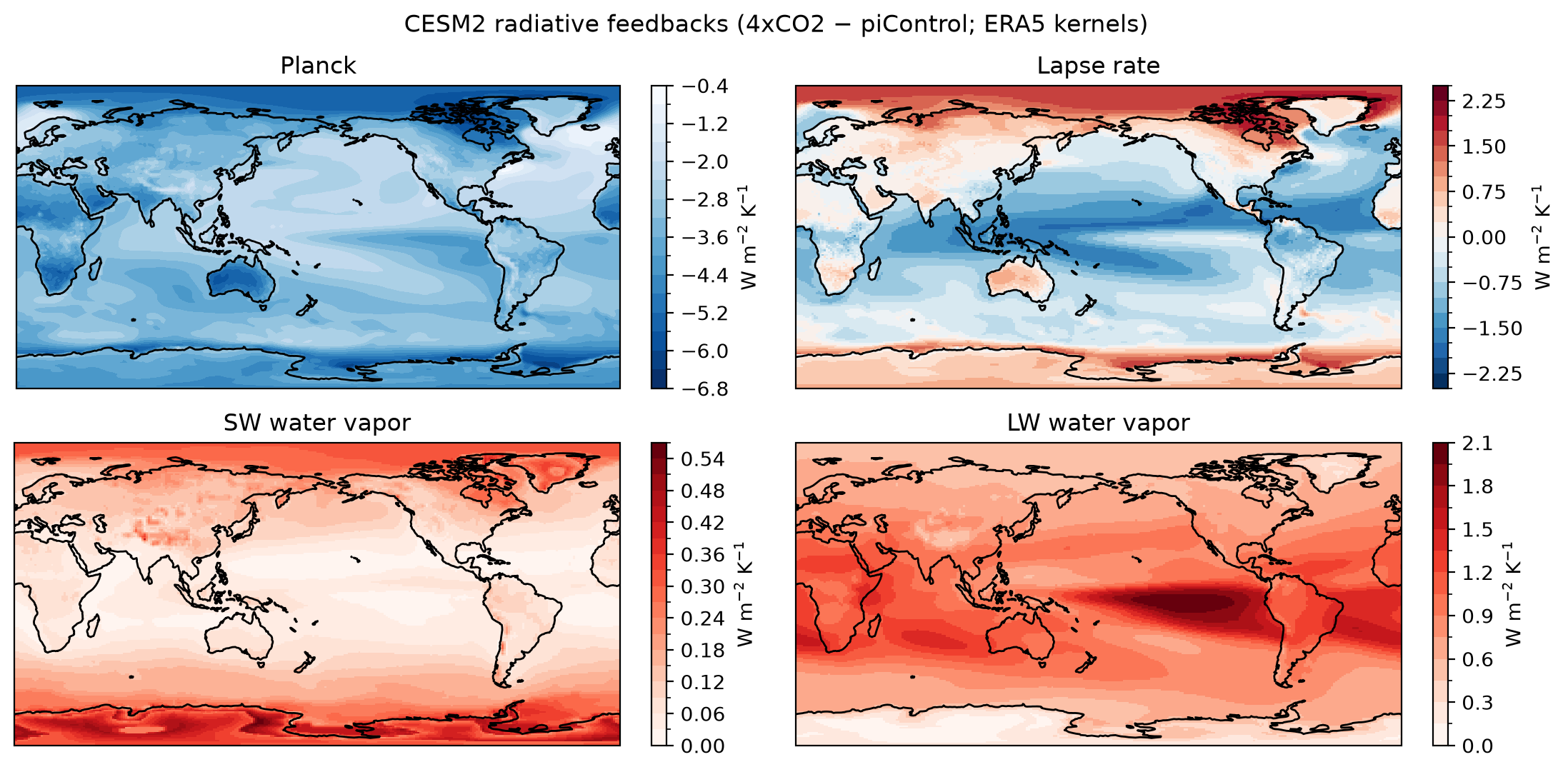
ann_dSWCRE = dSWCRE.mean(dim='month').load()
ann_dLWCRE = dLWCRE.mean(dim='month').load()Could not determine bucket type for bucket name cmip6: Your default credentials were not found. To set up Application Default Credentials, see https://cloud.google.com/docs/authentication/external/set-up-adc for more information., falling back to GCSFileSystem
Could not determine bucket type for bucket name cmip6: Your default credentials were not found. To set up Application Default Credentials, see https://cloud.google.com/docs/authentication/external/set-up-adc for more information., falling back to GCSFileSystem
Could not determine bucket type for bucket name cmip6: Your default credentials were not found. To set up Application Default Credentials, see https://cloud.google.com/docs/authentication/external/set-up-adc for more information., falling back to GCSFileSystem
Could not determine bucket type for bucket name cmip6: Your default credentials were not found. To set up Application Default Credentials, see https://cloud.google.com/docs/authentication/external/set-up-adc for more information., falling back to GCSFileSystem
Could not determine bucket type for bucket name cmip6: Your default credentials were not found. To set up Application Default Credentials, see https://cloud.google.com/docs/authentication/external/set-up-adc for more information., falling back to GCSFileSystem
Could not determine bucket type for bucket name cmip6: Your default credentials were not found. To set up Application Default Credentials, see https://cloud.google.com/docs/authentication/external/set-up-adc for more information., falling back to GCSFileSystem
Could not determine bucket type for bucket name cmip6: Your default credentials were not found. To set up Application Default Credentials, see https://cloud.google.com/docs/authentication/external/set-up-adc for more information., falling back to GCSFileSystem
Could not determine bucket type for bucket name cmip6: Your default credentials were not found. To set up Application Default Credentials, see https://cloud.google.com/docs/authentication/external/set-up-adc for more information., falling back to GCSFileSystem
Could not determine bucket type for bucket name cmip6: Your default credentials were not found. To set up Application Default Credentials, see https://cloud.google.com/docs/authentication/external/set-up-adc for more information., falling back to GCSFileSystem
Could not determine bucket type for bucket name cmip6: Your default credentials were not found. To set up Application Default Credentials, see https://cloud.google.com/docs/authentication/external/set-up-adc for more information., falling back to GCSFileSystem
Could not determine bucket type for bucket name cmip6: Your default credentials were not found. To set up Application Default Credentials, see https://cloud.google.com/docs/authentication/external/set-up-adc for more information., falling back to GCSFileSystem
Could not determine bucket type for bucket name cmip6: Your default credentials were not found. To set up Application Default Credentials, see https://cloud.google.com/docs/authentication/external/set-up-adc for more information., falling back to GCSFileSystem
Could not determine bucket type for bucket name cmip6: Your default credentials were not found. To set up Application Default Credentials, see https://cloud.google.com/docs/authentication/external/set-up-adc for more information., falling back to GCSFileSystem
Could not determine bucket type for bucket name cmip6: Your default credentials were not found. To set up Application Default Credentials, see https://cloud.google.com/docs/authentication/external/set-up-adc for more information., falling back to GCSFileSystem
Could not determine bucket type for bucket name cmip6: Your default credentials were not found. To set up Application Default Credentials, see https://cloud.google.com/docs/authentication/external/set-up-adc for more information., falling back to GCSFileSystem
Could not determine bucket type for bucket name cmip6: Your default credentials were not found. To set up Application Default Credentials, see https://cloud.google.com/docs/authentication/external/set-up-adc for more information., falling back to GCSFileSystem
Could not determine bucket type for bucket name cmip6: Your default credentials were not found. To set up Application Default Credentials, see https://cloud.google.com/docs/authentication/external/set-up-adc for more information., falling back to GCSFileSystem
Could not determine bucket type for bucket name cmip6: Your default credentials were not found. To set up Application Default Credentials, see https://cloud.google.com/docs/authentication/external/set-up-adc for more information., falling back to GCSFileSystem
Could not determine bucket type for bucket name cmip6: Your default credentials were not found. To set up Application Default Credentials, see https://cloud.google.com/docs/authentication/external/set-up-adc for more information., falling back to GCSFileSystem
Could not determine bucket type for bucket name cmip6: Your default credentials were not found. To set up Application Default Credentials, see https://cloud.google.com/docs/authentication/external/set-up-adc for more information., falling back to GCSFileSystem
Could not determine bucket type for bucket name cmip6: Your default credentials were not found. To set up Application Default Credentials, see https://cloud.google.com/docs/authentication/external/set-up-adc for more information., falling back to GCSFileSystem
Could not determine bucket type for bucket name cmip6: Your default credentials were not found. To set up Application Default Credentials, see https://cloud.google.com/docs/authentication/external/set-up-adc for more information., falling back to GCSFileSystem
Could not determine bucket type for bucket name cmip6: Your default credentials were not found. To set up Application Default Credentials, see https://cloud.google.com/docs/authentication/external/set-up-adc for more information., falling back to GCSFileSystem
Could not determine bucket type for bucket name cmip6: Your default credentials were not found. To set up Application Default Credentials, see https://cloud.google.com/docs/authentication/external/set-up-adc for more information., falling back to GCSFileSystem
Could not determine bucket type for bucket name cmip6: Your default credentials were not found. To set up Application Default Credentials, see https://cloud.google.com/docs/authentication/external/set-up-adc for more information., falling back to GCSFileSystem
Could not determine bucket type for bucket name cmip6: Your default credentials were not found. To set up Application Default Credentials, see https://cloud.google.com/docs/authentication/external/set-up-adc for more information., falling back to GCSFileSystem
Could not determine bucket type for bucket name cmip6: Your default credentials were not found. To set up Application Default Credentials, see https://cloud.google.com/docs/authentication/external/set-up-adc for more information., falling back to GCSFileSystem
Could not determine bucket type for bucket name cmip6: Your default credentials were not found. To set up Application Default Credentials, see https://cloud.google.com/docs/authentication/external/set-up-adc for more information., falling back to GCSFileSystem
Could not determine bucket type for bucket name cmip6: Your default credentials were not found. To set up Application Default Credentials, see https://cloud.google.com/docs/authentication/external/set-up-adc for more information., falling back to GCSFileSystem
Could not determine bucket type for bucket name cmip6: Your default credentials were not found. To set up Application Default Credentials, see https://cloud.google.com/docs/authentication/external/set-up-adc for more information., falling back to GCSFileSystem
Could not determine bucket type for bucket name cmip6: Your default credentials were not found. To set up Application Default Credentials, see https://cloud.google.com/docs/authentication/external/set-up-adc for more information., falling back to GCSFileSystem
Could not determine bucket type for bucket name cmip6: Your default credentials were not found. To set up Application Default Credentials, see https://cloud.google.com/docs/authentication/external/set-up-adc for more information., falling back to GCSFileSystem
Could not determine bucket type for bucket name cmip6: Your default credentials were not found. To set up Application Default Credentials, see https://cloud.google.com/docs/authentication/external/set-up-adc for more information., falling back to GCSFileSystem
Could not determine bucket type for bucket name cmip6: Your default credentials were not found. To set up Application Default Credentials, see https://cloud.google.com/docs/authentication/external/set-up-adc for more information., falling back to GCSFileSystem
Could not determine bucket type for bucket name cmip6: Your default credentials were not found. To set up Application Default Credentials, see https://cloud.google.com/docs/authentication/external/set-up-adc for more information., falling back to GCSFileSystem
Could not determine bucket type for bucket name cmip6: Your default credentials were not found. To set up Application Default Credentials, see https://cloud.google.com/docs/authentication/external/set-up-adc for more information., falling back to GCSFileSystem
Could not determine bucket type for bucket name cmip6: Your default credentials were not found. To set up Application Default Credentials, see https://cloud.google.com/docs/authentication/external/set-up-adc for more information., falling back to GCSFileSystem
Could not determine bucket type for bucket name cmip6: Your default credentials were not found. To set up Application Default Credentials, see https://cloud.google.com/docs/authentication/external/set-up-adc for more information., falling back to GCSFileSystem
Could not determine bucket type for bucket name cmip6: Your default credentials were not found. To set up Application Default Credentials, see https://cloud.google.com/docs/authentication/external/set-up-adc for more information., falling back to GCSFileSystem
Could not determine bucket type for bucket name cmip6: Your default credentials were not found. To set up Application Default Credentials, see https://cloud.google.com/docs/authentication/external/set-up-adc for more information., falling back to GCSFileSystem
Could not determine bucket type for bucket name cmip6: Your default credentials were not found. To set up Application Default Credentials, see https://cloud.google.com/docs/authentication/external/set-up-adc for more information., falling back to GCSFileSystem
Could not determine bucket type for bucket name cmip6: Your default credentials were not found. To set up Application Default Credentials, see https://cloud.google.com/docs/authentication/external/set-up-adc for more information., falling back to GCSFileSystem
Could not determine bucket type for bucket name cmip6: Your default credentials were not found. To set up Application Default Credentials, see https://cloud.google.com/docs/authentication/external/set-up-adc for more information., falling back to GCSFileSystem
Could not determine bucket type for bucket name cmip6: Your default credentials were not found. To set up Application Default Credentials, see https://cloud.google.com/docs/authentication/external/set-up-adc for more information., falling back to GCSFileSystem
Could not determine bucket type for bucket name cmip6: Your default credentials were not found. To set up Application Default Credentials, see https://cloud.google.com/docs/authentication/external/set-up-adc for more information., falling back to GCSFileSystem
Could not determine bucket type for bucket name cmip6: Your default credentials were not found. To set up Application Default Credentials, see https://cloud.google.com/docs/authentication/external/set-up-adc for more information., falling back to GCSFileSystem
Could not determine bucket type for bucket name cmip6: Your default credentials were not found. To set up Application Default Credentials, see https://cloud.google.com/docs/authentication/external/set-up-adc for more information., falling back to GCSFileSystem
Could not determine bucket type for bucket name cmip6: Your default credentials were not found. To set up Application Default Credentials, see https://cloud.google.com/docs/authentication/external/set-up-adc for more information., falling back to GCSFileSystem
Could not determine bucket type for bucket name cmip6: Your default credentials were not found. To set up Application Default Credentials, see https://cloud.google.com/docs/authentication/external/set-up-adc for more information., falling back to GCSFileSystem
Could not determine bucket type for bucket name cmip6: Your default credentials were not found. To set up Application Default Credentials, see https://cloud.google.com/docs/authentication/external/set-up-adc for more information., falling back to GCSFileSystem
Could not determine bucket type for bucket name cmip6: Your default credentials were not found. To set up Application Default Credentials, see https://cloud.google.com/docs/authentication/external/set-up-adc for more information., falling back to GCSFileSystem
Could not determine bucket type for bucket name cmip6: Your default credentials were not found. To set up Application Default Credentials, see https://cloud.google.com/docs/authentication/external/set-up-adc for more information., falling back to GCSFileSystem
Could not determine bucket type for bucket name cmip6: Your default credentials were not found. To set up Application Default Credentials, see https://cloud.google.com/docs/authentication/external/set-up-adc for more information., falling back to GCSFileSystem
Could not determine bucket type for bucket name cmip6: Your default credentials were not found. To set up Application Default Credentials, see https://cloud.google.com/docs/authentication/external/set-up-adc for more information., falling back to GCSFileSystem
Could not determine bucket type for bucket name cmip6: Your default credentials were not found. To set up Application Default Credentials, see https://cloud.google.com/docs/authentication/external/set-up-adc for more information., falling back to GCSFileSystem
Could not determine bucket type for bucket name cmip6: Your default credentials were not found. To set up Application Default Credentials, see https://cloud.google.com/docs/authentication/external/set-up-adc for more information., falling back to GCSFileSystem
Could not determine bucket type for bucket name cmip6: Your default credentials were not found. To set up Application Default Credentials, see https://cloud.google.com/docs/authentication/external/set-up-adc for more information., falling back to GCSFileSystem
Could not determine bucket type for bucket name cmip6: Your default credentials were not found. To set up Application Default Credentials, see https://cloud.google.com/docs/authentication/external/set-up-adc for more information., falling back to GCSFileSystem
Could not determine bucket type for bucket name cmip6: Your default credentials were not found. To set up Application Default Credentials, see https://cloud.google.com/docs/authentication/external/set-up-adc for more information., falling back to GCSFileSystem
Could not determine bucket type for bucket name cmip6: Your default credentials were not found. To set up Application Default Credentials, see https://cloud.google.com/docs/authentication/external/set-up-adc for more information., falling back to GCSFileSystem
Could not determine bucket type for bucket name cmip6: Your default credentials were not found. To set up Application Default Credentials, see https://cloud.google.com/docs/authentication/external/set-up-adc for more information., falling back to GCSFileSystem
Could not determine bucket type for bucket name cmip6: Your default credentials were not found. To set up Application Default Credentials, see https://cloud.google.com/docs/authentication/external/set-up-adc for more information., falling back to GCSFileSystem
Could not determine bucket type for bucket name cmip6: Your default credentials were not found. To set up Application Default Credentials, see https://cloud.google.com/docs/authentication/external/set-up-adc for more information., falling back to GCSFileSystem
Could not determine bucket type for bucket name cmip6: Your default credentials were not found. To set up Application Default Credentials, see https://cloud.google.com/docs/authentication/external/set-up-adc for more information., falling back to GCSFileSystem
fig2, axs2 = plt.subplots(1, 2, figsize=(11, 2.5), dpi=200, subplot_kw=dict(projection=pc180), layout='constrained')
ann_dSWCRE.plot.contourf(ax=axs2[0], levels=21, cbar_kwargs=dict(label='W m$^{-2}$'), transform=pc0)
ann_dLWCRE.plot(ax=axs2[1], levels=21, cbar_kwargs=dict(label='W m$^{-2}$'), transform=pc0)
for ax in axs2.flatten():
ax.coastlines()
axs2[0].set_title('SW')
axs2[1].set_title('LW')
fig2.suptitle('CESM2 $\\Delta$CRE (4xCO2 $-$ piControl)', y=1.05)