Introduction to Argo Observations¶

Overview¶

Argo floats are autonomous profiling instruments that sample the interior ocean by traveling with the ocean currents. They are part of the Argo program, an international collaborative effort to monitor the state of the ocean. The deployment of thousands of Argo floats has enabled new observation-based studies in previously undersampled regions (e.g. Wong et al. 2020, Swart et al. 2023). Some newer Argo floats, known as Biogeochemical-Argo (BGC-Argo) floats, have been further equipped with biologically relevant sensors for oxygen, nitrate, optical backscatter, and chlorophyll fluorescence (Claustre et al. 2020, Sarmiento et al. 2023, Roemmich et al. 2019). Argo floats provide critical data that enhances our understanding of the ocean and its influence on the global climate system. Through international collaboration and advanced technology, the Argo program plays a vital role in monitoring and studying the world’s oceans.

Here, we introduce Argo profiling floats, which are autonomous instruments that operate remotely and sample the ocean interior continuously. Our objectives:

What are Argo floats?
How are the data formatted?
How can we transform data to work with?
What are some ways of visualizing float data?

In the next notebook, Accessing Argo Data, we will explore different ways of downloading and retrieving float profiles.

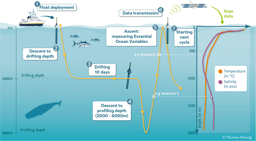
Basic profiling scheme of an Argo float¶

from IPython.display import Image
print('Float Cycle Diagram, courtesy of UCSD (https://argo.ucsd.edu/how-do-floats-work/) ')
Image(filename='../images/float_cycle_diagram.png')

Float Cycle Diagram, courtesy of UCSD (https://argo.ucsd.edu/how-do-floats-work/)

Prerequisites (fill in)¶

Concepts	Importance	Notes
Intro to NetCDF	Necessary	Familiarity with metadata structure
Intro to Xarray	Necessary
Intro to Matplotlib	Helpful

Time to learn: 15 min

Imports¶

Begin your body of content with another --- divider before continuing into this section, then remove this body text and populate the following code cell with all necessary Python imports up-front:

# Import packages
import sys
import os
import numpy as np
import pandas as pd
import scipy
import xarray as xr
from datetime import datetime, timedelta

import matplotlib.pyplot as plt
import matplotlib.colors as mcolors
import seaborn as sns
from cmocean import cm as cmo

How is Argo data formatted?¶

In the next notebook, we will discuss other ways of accessing Argo data. Here, we will use one float as an example for what the platform is observing.

Often, floats are packaged into xarray Datasets, which are objects that can deal with data with multiple dimensions.

wmo = 5905367
flt_data = xr.open_dataset('../data/' + str(wmo) + '_Sprof.nc', decode_times=False)
flt_data

Note that the “Attributes” of the .nc file show metadata on the platform. We can also look at more specific attributes of variables.

Most users should always use the *_ADJUSTED values. The corresponding variable *_ADJUSTED_QC gives the standard Argo QC flags.

flt_data.TEMP_ADJUSTED

Plotting time-depth sections from a single float.¶

fig = flt_data.TEMP.T.plot(figsize = (6,3), cmap = cmo.thermal)
ax = plt.gca()
ax.invert_yaxis()
ax.set_title('Adjusted Temperature from WMO ' + str(wmo))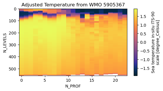

Transforming an Xarray Dataset into a Pandas Dataframe.¶

The pd Dataframe is a useful object resembling a table (can be interchangeable with .csv files).
After transforming to a Dataframe, we can easily pull variables of interest, and add others.
Note that having time in a numerical format (here, “yearday” since 2019-01-01) helps with training models.

# Choose variables to use
float_df = flt_data[['JULD','LATITUDE', 'LONGITUDE','PRES_ADJUSTED','TEMP_ADJUSTED','PSAL_ADJUSTED',
                         'DOXY_ADJUSTED','NITRATE_ADJUSTED', # , 'PH_IN_SITU_TOTAL_ADJUSTED','BBP700_ADJUSTED', 
                        'JULD_QC', 'POSITION_QC', 'PRES_ADJUSTED_QC', 'TEMP_ADJUSTED_QC','PSAL_ADJUSTED_QC', 
                        'DOXY_ADJUSTED_QC', 'NITRATE_ADJUSTED_QC']].to_dataframe() #'BBP700_ADJUSTED_QC' #, 'PH_IN_SITU_TOTAL_ADJUSTED_QC',
dtimes = pd.to_datetime(float_df.JULD.values, unit='D', origin=pd.Timestamp('1950-01-01'))

def datetime2ytd(time):
    """ Return time in YTD format from datetime format.
    Sometimes easier to work with numerical date values."""
    return (time - np.datetime64('2019-01-01'))/np.timedelta64(1, 'D')
float_df['YEARDAY'] = datetime2ytd(dtimes)

# Make a profile ID for each profile
prof = float_df.index.get_level_values(0)
prof = prof.astype(str); prof = [tag.zfill(3) for tag in prof]
float_df['PROFID'] = [str(wmo)+tag for tag in prof]


# Convert QC flags to integers
qc_keys = ['JULD_QC', 'POSITION_QC', 'PRES_ADJUSTED_QC', 'TEMP_ADJUSTED_QC', 'PSAL_ADJUSTED_QC',
    'DOXY_ADJUSTED_QC', 'NITRATE_ADJUSTED_QC'] #, 'PH_IN_SITU_TOTAL_ADJUSTED_QC', 'BBP700_ADJUSTED_QC']
for key in qc_keys:  #qc flags are not stored as ints so we can convert
        newlist = []
        for qc in float_df[key]:
                if str(qc)[2] == 'n': newlist.append('NaN')
                else: newlist.append(str(qc)[2])
        float_df[key] = newlist

Here is what the resulting dataframe might look like:

float_df

Considering dive-averaged data¶

The sampling strategy of the float is to sample as it ascends from a dive. If we want to know the average information for the entire dive, we can average over the dive observations.

def list_profile_DFs(df):
    """ 
    @param df: dataframe with all profiles
    @return: list of dataframes, each with a unique profile
    """
    PROFIDs = pd.unique(df.PROFID)
    profile_DFs = []
    for i in range(len(PROFIDs)):
        profile_DFs.append(df[df['PROFID']==PROFIDs[i]].copy())
    return profile_DFs


def make_diveav(df):
    """
    Make dive-averaged dataframes (per profile). 
    @param:    df: dataframe with all profiles
    @return:   single dataframe with dive-averaged data
    """
    prof_list = list_profile_DFs(df)

    newDF = pd.DataFrame()
    newDF['PROFID'] = pd.unique(df.PROFID)
    newDF['YEARDAY'] = [np.nanmean(x.YEARDAY) for x in prof_list]
    newDF['LATITUDE'] = [x.LATITUDE.mean() for x in prof_list]
    newDF['LONGITUDE'] = [x.LONGITUDE.mean() for x in prof_list]

    return newDF

This particular float returns 23 profiles in the bounds we provided earlier.

float_dav = make_diveav(float_df)
float_dav

Using the dive-averaged data, we can easily plot the overall trajectory using matplotlib.

# plot with float trajectory

fig = plt.figure(figsize=(10,4))
ax = fig.gca()

sca = ax.scatter(float_dav.LONGITUDE, float_dav.LATITUDE, c=float_dav.YEARDAY, cmap='viridis', s=20, zorder=3)
ax.plot(float_dav.LONGITUDE, float_dav.LATITUDE, zorder=1, linewidth=0.5, linestyle='dashed', color='k')
plt.colorbar(sca, shrink=0.6, label='Days since 2019-01-01')

ax.yaxis.set_major_formatter("{x:1.0f}°S")
ax.xaxis.set_major_formatter("{x:1.0f}°E")
ax.set_aspect('equal')
ax.grid(zorder=1)
ax.set_ylim([-68, -60])

ax.set_title('Float ' + str(wmo) + ' Trajectory in 2019')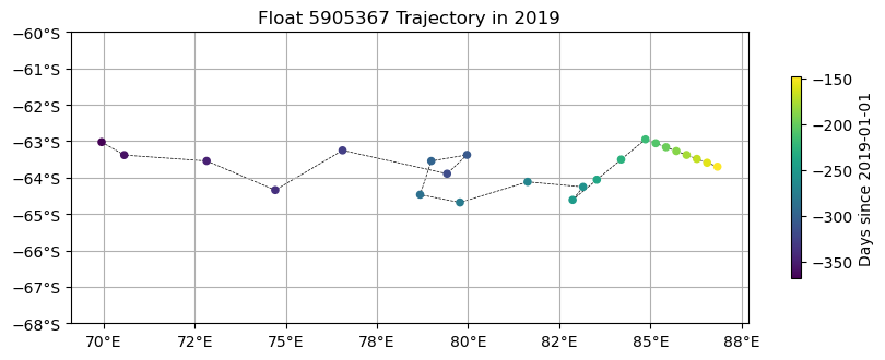

In the next notebook, Accessing Argo, we go over more details on accessing the Argo data and plotting profiles.

Summary¶

Add one final --- marking the end of your body of content, and then conclude with a brief single paragraph summarizing at a high level the key pieces that were learned and how they tied to your objectives. Look to reiterate what the most important takeaways were.

What’s next?¶

Let Jupyter book tie this to the next (sequential) piece of content that people could move on to down below and in the sidebar. However, if this page uniquely enables your reader to tackle other nonsequential concepts throughout this book, or even external content, link to it here!

Resources and references¶

Finally, be rigorous in your citations and references as necessary. Give credit where credit is due. Also, feel free to link to relevant external material, further reading, documentation, etc. Then you’re done! Give yourself a quick review, a high five, and send us a pull request. A few final notes:

Kernel > Restart Kernel and Run All Cells... to confirm that your notebook will cleanly run from start to finish
Kernel > Restart Kernel and Clear All Outputs... before committing your notebook, our machines will do the heavy lifting
Take credit! Provide author contact information if you’d like; if so, consider adding information here at the bottom of your notebook
Give credit! Attribute appropriate authorship for referenced code, information, images, etc.
Only include what you’re legally allowed: no copyright infringement or plagiarism

Thank you for your contribution!

Preamble

How to Cite This Cookbook

Argo Foundations

Accessing Argo Data