Accessing SnowEx Data using the snowexsql database

Overview¶

The SnowExSQL database is a PostgreSQL/PostGIS database hosted on AWS, holding snow observations from NASA SnowEx field campaigns spanning 2017–2023. It contains snow pit profiles, manual depth transects, ground-penetrating radar (GPR), snow microstructure (SMP), and more.

This tutorial introduces the SnowEx Lambda client — the current recommended way to access the database. The Lambda client uses a public HTTPS endpoint, so you do not need AWS credentials, a VPN, or any special configuration. Database security is handled behind the scenes by AWS.

This tutorial covers:

Connecting to the SnowEx database
Discovering what data is available
Querying data by geographic area of interest
Filtering by campaign and year
Point data and layer data: understanding the difference

Prerequisites¶

Concepts	Importance	Notes
Basic Python and pandas	Necessary
Introduction to GeoPandas	Helpful	Familiarity with GeoDataFrames
NASA SnowEx field campaigns	Helpful	See Field Campaigns Overview

Time to learn: ~30 minutes

Imports¶

from datetime import date

import contextily as ctx
import geopandas as gpd
import matplotlib.pyplot as plt
import numpy as np
import pandas as pd
from shapely.geometry import box, Point

from snowexsql.lambda_client import SnowExLambdaClient

Connecting to the SnowEx Database¶

The SnowExLambdaClient connects to the SnowEx database through a public AWS Lambda Function URL. There is nothing to configure — just instantiate the client and go.

client = SnowExLambdaClient()

# Get the two main measurement classes
classes = client.get_measurement_classes()
PointMeasurements = classes['PointMeasurements']
LayerMeasurements = classes['LayerMeasurements']

# Verify the connection
result = client.test_connection()
print(f"Connected: {result.get('connected', False)}")

Connected: True

Discovering What Data Is Available¶

Before querying, it’s useful to explore what measurement types and campaigns are in the database. Each class exposes all_* properties that return lists of available values.

print("Layer measurement types:", LayerMeasurements.all_types)

Layer measurement types: ['density', 'grain_size', 'grain_type', 'hand_hardness', 'manual_wetness', 'comments', 'permittivity', 'liquid_water_content', 'snow_temperature', 'force', 'sample_signal', 'reflectance', 'specific_surface_area', 'equivalent_diameter']

print("Point measurement types:", PointMeasurements.all_types)

Point measurement types: ['two_way_travel', 'depth', 'swe', 'density']

print("Available instruments:", PointMeasurements.all_instruments)

Available instruments: ['camera', 'gpr', 'magnaprobe', 'mesa', 'pit ruler']

Other discovery properties follow the same pattern. For example, LayerMeasurements.all_dates returns every distinct measurement date, all_observers returns observer names, and all_dois returns citable dataset identifiers. These are useful for understanding the full scope of the database before constructing a query.

Point Data and Layer Data: Understanding the Difference¶

The two data types have different structures:

	PointMeasurements	LayerMeasurements
Table	`points`	`layers`
What it represents	A single value at a single location	A value at a specific depth within the snowpack
`value` column type	Float (numeric)	Text (requires conversion)
Geometry	Direct on each record	From the parent `Site` record
Example data	Magnaprobe snow depths, GPR travel times	Snow temperature profiles, density profiles, grain size

Querying Data by Area of Interest¶

A common use case is: “I have a region of interest — what SnowEx data exists there?”

Both PointMeasurements and LayerMeasurements support from_area(), which accepts a Shapely polygon and returns a GeoDataFrame of all matching records.

Layer Data¶

Here we query snow temperature profiles collected in the Boise Basin, Idaho area.

# Define a bounding box in WGS84 (longitude/latitude)
bbox = box(minx=-116.14, miny=43.73, maxx=-116.04, maxy=43.8)
bbox_gdf = gpd.GeoDataFrame([1], geometry=[bbox], crs='EPSG:4326')

df_layer = LayerMeasurements.from_area(
    shp=bbox,
    date_greater_equal=date(2020, 1, 1),
    date_less_equal=date(2022, 12, 30),
    crs=4326,
    type='snow_temperature',
    limit=600,
    verbose=True,
)
print(f"Retrieved {len(df_layer)} records")
df_layer.head()

Retrieved 586 records

fig, ax = plt.subplots(figsize=(10, 8))

df_layer.to_crs(epsg=3857).plot(
    ax=ax, color='steelblue', markersize=25, alpha=0.7, label='Layer data'
)
bbox_gdf.to_crs(epsg=3857).boundary.plot(
    ax=ax, color='red', linewidth=2, label='Query area'
)
ctx.add_basemap(ax, source=ctx.providers.OpenStreetMap.Mapnik, alpha=0.6)
ax.set_title(f'Snow Temperature Measurements — Boise Basin (n={len(df_layer)})')
ax.set_xlabel('Easting')
ax.set_ylabel('Northing')
ax.legend()
plt.tight_layout()
plt.show()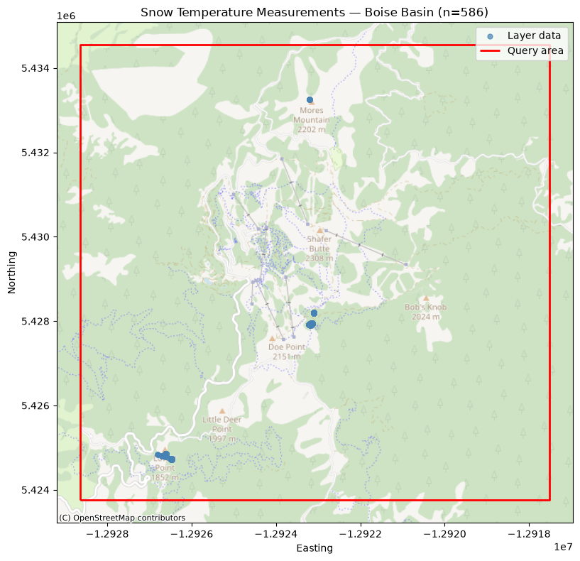

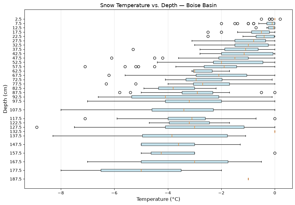
Layer Depth Profile¶

Because LayerMeasurements.value is stored as Text, we must convert it to numeric before plotting or computing statistics. Here we visualize the snow temperature profile data from Boise Basin as a boxplot by depth band.

# Convert value to numeric (required for LayerMeasurements)
df_layer['value'] = pd.to_numeric(df_layer['value'], errors='coerce')
df_layer = df_layer.dropna(subset=['value', 'depth'])

# Create 5 cm depth bands
bin_width = 5.0
bins = np.arange(
    np.floor(df_layer['depth'].min()),
    np.ceil(df_layer['depth'].max()) + bin_width,
    bin_width,
)
df_layer['depth_band'] = pd.cut(
    df_layer['depth'],
    bins=bins,
    labels=bins[:-1] + bin_width / 2,
    include_lowest=True,
)
depth_bands = sorted(df_layer['depth_band'].dropna().unique())
data_by_band = [
    df_layer[df_layer['depth_band'] == b]['value'].values for b in depth_bands
]

fig, ax = plt.subplots(figsize=(10, 7))
bp = ax.boxplot(
    data_by_band, positions=depth_bands, vert=False,
    patch_artist=True, widths=3.0,
)
for patch in bp['boxes']:
    patch.set_facecolor('lightblue')
    patch.set_alpha(0.7)

ax.invert_yaxis()
ax.set_xlabel('Temperature (°C)', fontsize=12)
ax.set_ylabel('Depth (cm)', fontsize=12)
ax.set_title('Snow Temperature vs. Depth — Boise Basin', fontsize=13)
ax.grid(True, alpha=0.3, axis='x')
plt.tight_layout()
plt.show()

Point Data¶

Now we query snow depth point measurements on Grand Mesa, Colorado.

bbox_gm = box(minx=-108.195487, miny=39.031819, maxx=-108.189329, maxy=39.036568)
bbox_gm_gdf = gpd.GeoDataFrame([1], geometry=[bbox_gm], crs='EPSG:4326')

df_point = PointMeasurements.from_area(
    shp=bbox_gm,
    crs=4326,
    type='depth',
    limit=5000,
)
print(f"Retrieved {len(df_point)} records")
df_point.head()

Retrieved 5000 records

verbose=True returns richer metadata for point measurements — campaign name, instrument, and observer — useful for attribution and cross-referencing.

df_point_v = PointMeasurements.from_area(
    shp=bbox_gm,
    crs=4326,
    type='depth',
    limit=5,
    verbose=True,
)
df_point_v[['value', 'campaign_name', 'instrument_name', 'observer_name']]

fig, ax = plt.subplots(figsize=(10, 8))

df_point.to_crs(epsg=3857).plot(
    ax=ax,
    column='value',
    cmap='viridis',
    markersize=30,
    alpha=0.7,
    legend=True,
    legend_kwds={'label': 'Snow Depth (cm)', 'shrink': 0.8},
)
bbox_gm_gdf.to_crs(epsg=3857).boundary.plot(
    ax=ax, color='red', linewidth=2, label='Query area'
)
ctx.add_basemap(ax, source=ctx.providers.OpenStreetMap.Mapnik, alpha=0.6)
ax.set_title(f'Snow Depth — Grand Mesa (n={len(df_point)})')
ax.set_xlabel('Easting')
ax.set_ylabel('Northing')
ax.legend(loc='upper left')
plt.tight_layout()
plt.show()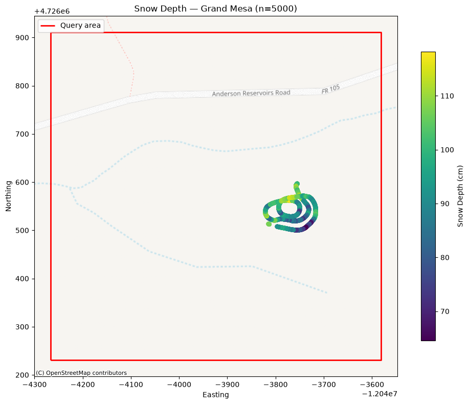

A histogram shows the distribution of snow depths across the queried area.

fig, ax = plt.subplots(figsize=(8, 4))
ax.hist(df_point['value'].dropna(), bins=30, color='steelblue', edgecolor='white')
ax.set_xlabel('Snow Depth (cm)')
ax.set_ylabel('Count')
ax.set_title(f'Snow Depth Distribution — Grand Mesa (n={len(df_point)})')
ax.axvline(df_point['value'].median(), color='orange', linestyle='--',
           label=f"Median: {df_point['value'].median():.1f} cm")
ax.legend()
plt.tight_layout()
plt.show()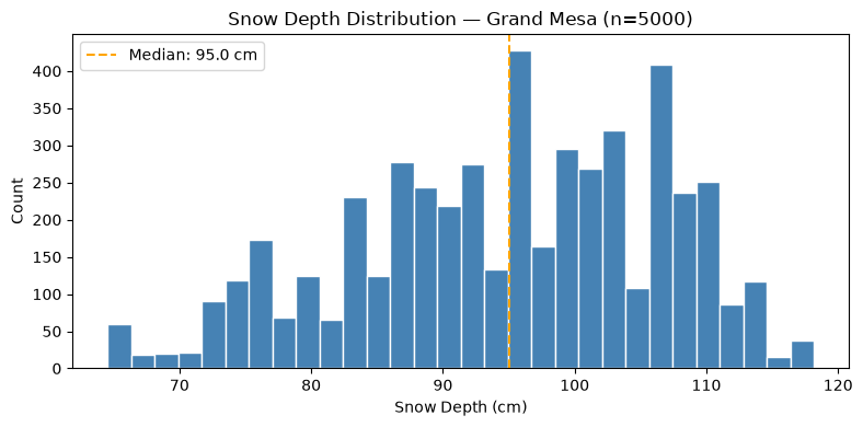

Querying by Point and Radius¶

If you have a specific site location rather than a bounding box, pass a Point geometry and a buffer radius (in the units of the CRS — degrees for EPSG:4326, meters for a projected CRS).

# Center point of the Grand Mesa query area (lon, lat)
site_pt = Point(-108.192, 39.034)

df_pt_buf = PointMeasurements.from_area(
    pt=site_pt,
    buffer=0.005,   # ~500 m in degrees at this latitude
    crs=4326,
    type='depth',
    limit=1000,
)
print(f"Retrieved {len(df_pt_buf)} records within radius")
df_pt_buf.head()

Retrieved 1000 records within radius

Filtering by Campaign and Year¶

When you already know which SnowEx campaign or time period you’re interested in, use from_filter() to query the entire database without specifying a geographic area.

We can list all the campaigns currently stored in the database:

print("Campaigns in the database:", LayerMeasurements.all_campaigns)

Campaigns in the database: ['North Slope', '2021 Timeseries', 'Alaska 2023', 'Fairbanks', '2020 Timeseries', 'Grand Mesa']

df_campaign = PointMeasurements.from_filter(
    campaign='Alaska 2023',
    type='depth',
    limit=1000,
)
print(f"Retrieved {len(df_campaign)} records from Alaska 2023 campaign")
df_campaign.head()

Retrieved 1000 records from Alaska 2023 campaign

Filter by Date Range¶

df_year = LayerMeasurements.from_filter(
    date_greater_equal=date(2020, 1, 1),
    date_less_equal=date(2020, 12, 31),
    type='density',
    limit=500,
)
print(f"Retrieved {len(df_year)} density records from 2020")
df_year.head()

Retrieved 500 density records from 2020

Snow Water Equivalent (SWE)¶

Snow water equivalent is one of the primary variables SnowEx was designed to measure. It is available as a PointMeasurements type. Here we demonstrate querying Alaska swe data for a specific date range:

df_swe = PointMeasurements.from_filter(
    type='swe',
    campaign='Alaska 2023',
    date_greater_equal=date(2023, 3, 7),
    date_less_equal=date(2023, 3, 8),
    limit=5000,
    verbose=False,
)
print(f"Retrieved {len(df_swe)} SWE records")
df_swe.head()

Retrieved 5000 SWE records

fig, ax = plt.subplots(figsize=(10, 8))
df_swe.to_crs(epsg=3857).plot(
    ax=ax,
    column='value',
    cmap='Blues',
    markersize=20,
    alpha=0.7,
    legend=True,
    legend_kwds={'label': 'SWE (mm)', 'shrink': 0.8},
)
#ctx.add_basemap(ax, source=ctx.providers.OpenStreetMap.Mapnik, alpha=0.6)
ax.set_title(f'Snow Water Equivalent — Alaska 2023 Campaign, Mar 7-8 (n={len(df_swe)})')
ax.set_xlabel('Easting')
ax.set_ylabel('Northing')
plt.tight_layout()
plt.show()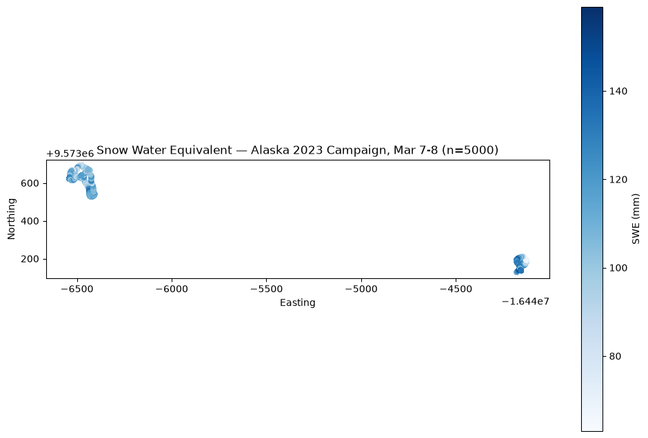

Resources and references¶

snowexsql on GitHub
SnowEx Field Campaigns Overview — background on what data was collected and where
GeoPandas documentation
Shapely documentation
contextily documentation