UXarray logo

Comparison to Xarray¶

In this tutorial, you’ll learn about:¶

The differences and similarities between UXarray’s and Xarray’s plotting routines
Using hvPlot with Xarray

UXarray Plotting User Guide

Prerequisites¶

Concepts	Importance	Notes
Xarray	Necessary

Time to learn: 5 minutes

Introduction¶

For users coming from an Xarray background, much of UXarray’s design is familiar. This notebook showcases an example of transitioning a visualization of a structured grid using Xarray into a visualization of an unstructured grid using UXarray.

import cartopy.crs as ccrs
import matplotlib.pyplot as plt
import uxarray as ux
import xarray as xr

Data¶

We use two variations of the outCSne30 grid for this example. One of them is the original unstructured cube sphere, with the other being a remapped structured version.

Xarray¶

base_path = "../../meshfiles/"
ds_path = base_path + "outCSne30.structured.nc"
xrds = xr.open_dataset(ds_path)
xrds

UXarray¶

base_path = "../../meshfiles/"
grid_filename = base_path + "outCSne30.grid.ug"
data_filename = base_path + "outCSne30.data.nc"

uxds = ux.open_dataset(grid_filename, data_filename)
uxds

Visualization¶

Xarray¶

xrds["psi"].plot(figsize=(12, 5), cmap="inferno")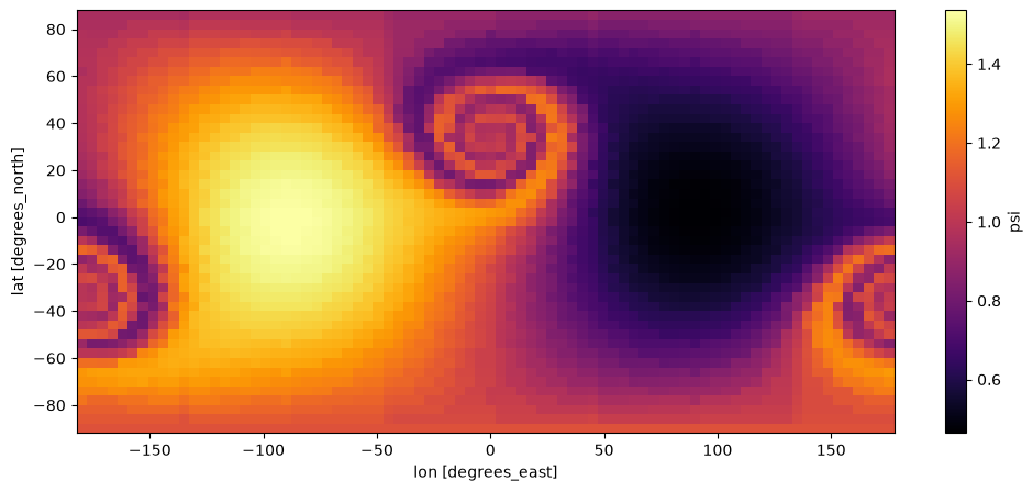

UXarray¶

uxds["psi"].plot(width=800, height=400, backend="matplotlib", cmap="inferno")

Using `hvPlot` to combine UXarray & Xarray Plots¶

Since UXarray is written using hvPlot, we can visualize Xarray and UXarray plots together by using hvplot.xarray.

See also:

To learn more about hvPlot and Xarray, please refer to the hvPlot Documentation

import holoviews as hv
import hvplot.xarray

hv.extension("bokeh")

(
    xrds.hvplot(cmap="inferno", title="Xarray with hvPlot", width=800, height=400)
    + uxds["psi"].plot(
        cmap="inferno",
        title="UXarray Plot",
        width=800,
        height=400,
        periodic_elements="split",
    )
).cols(1)

Plotting with UXarray

Visualizing High-Resolution Grids

Visualization Recipes

MPAS Atmosphere