Chapter 5: Real-time MRMS Visualization

Welcome to the Real-time MRMS Visualization notebook! In this workflow, you will receive a quick briefing on the Multi-Radar/Multi-Sensor System (MRMS) content covered in Chapter 1, learn about data access from Amazom Web Services (AWS), make a selection of MRMS data to request from AWS, and visualize the latest radar data in an interactive plot.

Intent: This Project Pythia notebook allows a user to gain familiarity with the process of requesting real-time MRMS data from AWS S3 and provides the opportunity for further learning.
Audience: Anyone with at least 5GB of memory on their computer or computing environment and a fundamental knowledge of MRMS. No programming experience is required to go run this notebook, but it will help you understand where this data is coming from.
Outcome: An interactive plot showing MRMS imagery from a selected region and radar product.
Time to Learn: 15 minutes to run the notebook and read the documentation; 30 minutes to become familiar enough with the material to replicate these methods.

Overview¶

Import required packages
Learn about MRMS
Explore near real-time MRMS data hosted on AWS
Select a region and product for viewing
Access selected MRMS data from AWS
Visualize a selected variable using an interactive plot

Imports¶

Here are all required Python packages to run this code.

# Packages required to request and open data from AWS S3
import s3fs
import urllib
import tempfile
import gzip
import xarray as xr

# Packages required for data visualization
import datetime
from datetime import timezone
import numpy.ma as ma
from metpy.plots import ctables
import numpy as np
import holoviews as hv
import pandas as pd
import panel as pn
import hvplot.xarray 
import matplotlib.colors as mcls
from matplotlib.colors import Normalize
#pn.extension("bokeh")
hv.extension('bokeh')

About MRMS¶

image

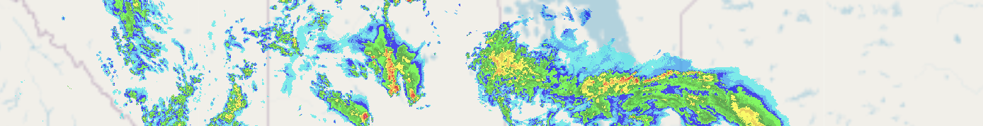
The Multi-Radar/Multi-Sensor System (MRMS) produces products for public infrastructure, weather forecasts and warnings, aviation, and numerical weather prediction. It provides high spatial (1-km) and temporal (2-min) resolution radar products at 31 vertical levels, and ingests data from numerous sources (including radar networks across the US and Canada, surface and upper air observations, lightning detection systems, satellite observations, and forecast models)¹

For more information, please refer to Chapter 1 of this project: Learning about MRMS.

About AWS and NODD¶

logo images

The Amazon Web Services Simple Storage Service (AWS S3) is cloud-based object storage service. Through a public-private partnership with the National Oceanic and Atmospheric Administration (NOAA)'s Open Data Dissemination Program (NODD), NOAA is able to store multiple petabytes of open-access earth science data on AWS S3, including the MRMS dataset. This allows users to quickly and freely access MRMS data in real-time (with an update frequency of two minutes) without having to download the data to their personal systems.

Because of this partnership, we can access the data as an anonymous client -- no login required!

# Initialize the S3 filesystem as anonymous
aws = s3fs.S3FileSystem(anon=True)

You can explore the S3 bucket that holds MRMS data to assess data availability and structure -- just visit this link, which takes you to the MRMS bucket.

# Here's a hint -- you can run aws.ls to see the file structure in code. Try it yourself!
aws.ls(f'noaa-mrms-pds/CONUS/', refresh=True)[0:5]

Data selection¶

For ease of use, I’ve integrated ipywidgets (drop-down menus!) that allow you to make selections from AWS, and refined a selection of data variables as a demonstration. You can choose between the QC’d Merged Reflectivity Composite (the maximum reflectivity in a column, as a composite), a 12-hour multisensor QPE from Pass 1 (12h rainfall accumulation estimate, using data from multiple sensors), and the Probability of Severe Hail (probability of 0.75-inch diameter hail).

Now, you have the option to select a region and a radar product to visualize in near real-time. Go ahead and use the drop-down menus to select a region, a radar product, then run the next cell. If you run the drop-down cell again, it will reset your values.

# Define dropdown options
region_options = ["CONUS", "ALASKA", "CARIB", "GUAM", "HAWAII"]
product_options = [
    "MergedReflectivityQCComposite_00.50",
    "MultiSensor_QPE_12H_Pass1_00.00",
    "POSH_00.50"
]

# Create the dropdowns with similar layout/formatting
region_choice = pn.widgets.Select(name='Region', options=region_options, width=325)
product_choice = pn.widgets.Select(name='MRMS product', options=product_options, width=325)

# Display the widgets together in a vertical layout (Column)
pn.Column(region_choice, product_choice)

Congratulations, you’ve made your data selection!

If you choose to adapt this notebook to your own workflow, this section can easily be adjusted to your own use case. Simply delete the cell above, then update the cell below to reflect the region and data variable you wish to use. If you decide to use a product that is not covered in this notebook, you can search through all available data products on AWS and paste it in verbatim. It may be helpful to cross-reference these variables against the NSSL variable table and Chapter 1.

# Retrieve the user selection from 'region' 
region = region_choice.value

# Retrieve the user selection from 'MRMS product'
product = product_choice.value

print(region, product)

Data request¶

Now that you’ve made your variable selection, it’s time to read in the data from AWS. First, we retrieve the current UTC datetime so that we can request files from today’s S3 bucket.

# Retrieve the current datetime in UTC to know which bucket to query
now = datetime.datetime.now(datetime.UTC)
datestring = now.strftime('%Y%m%d')

Next, we query the S3 bucket to make sure the data is available on AWS. If this section errors, reference the S3 bucket to confirm that your requested region, date, and product exists and is entered correctly.

# Query the S3 bucket for the available files that meet the criteria
try:
    data_files = aws.ls(f'noaa-mrms-pds/{region}/{product}/{datestring}/', refresh=True)  
except Exception as e:
    print(f"Error accessing S3 bucket: {e}")
    data_files = []

Finally, we make the data request and read it in using xarray. This block of code finds the most recent file that fits your criteria, ensures that the file was created recently (within two hours), then makes the data request. Due to way the data was uploaded to S3, the file arrives as a compressed grib2 file. This code decompresses the file and reads it in using xarray, making the format more easily incorporated into our workflow.

if data_files:
    # Choose the last file from S3 for the most recent data
    most_recent_file = data_files[-1]

    # Check that the most recent file is within 2 hours of current time
    timestamp_str = most_recent_file.split('_')[-1].replace('.grib2.gz', '')
    dt = datetime.datetime.strptime(timestamp_str, "%Y%m%d-%H%M%S").replace(tzinfo=timezone.utc)
    if abs((now - dt).total_seconds()) <= 120 * 60:
        # Download file to memory, decompress from .gz, and read into xarray
        try:
            response = urllib.request.urlopen(f"https://noaa-mrms-pds.s3.amazonaws.com/{most_recent_file[14:]}")
            compressed_file = response.read()

            with tempfile.NamedTemporaryFile(suffix=".grib2") as f:
                f.write(gzip.decompress(compressed_file))
                f.flush()
                data = xr.load_dataarray(f.name, engine="cfgrib", decode_timedelta=True)
        except Exception as e:
            print(f"Failed to process {product}: {e}")

Visualization¶

Now that we have the data read into memory using xarray, it is quite simple to plot. Here, we use hvplot to make an interactive visualization that allows the user to zoom in to a region of interest and mouse over values to better understand the product’s functionality over a specific region.

# Mask data for neater visualization
data = data.where(data > 0, np.nan)

# Get the NWS Reflectivity colormap and normalize range
ref_norm, ref_cmap = ctables.registry.get_with_steps('NWSReflectivity', 5, 5)

# Convert to hex colors for Bokeh
norm = Normalize(vmin=ref_norm.vmin, vmax=ref_norm.vmax)
hex_cmap = [ref_cmap(norm(val)) for val in range(ref_norm.vmin, ref_norm.vmax + 5, 5)]
hex_cmap = [mcls.to_hex(c) for c in hex_cmap]

# Plot using hvplot
reflectivity_plot = data.hvplot.image(
    x="longitude", y="latitude",
    cmap=hex_cmap,
    colorbar=True,
    geo=True, 
    tiles=True, 
    alpha=0.7,
    clim=(ref_norm.vmin, ref_norm.vmax),
    title=f"{product} - {pd.to_datetime(data.time.values).strftime('%b %d, %Y at %H:%M:%S')} UTC",
    frame_width=700,
    frame_height=500,
    xlabel='Longitude',
    ylabel='Latitude',
    tools=['hover']
)

reflectivity_plot

Above is your visualization! You can use the menu bar at the upper right side of the plot to pan around the plot, zoom in to a region of interest, and reset your selections to the default map. If you mouse over the values on the screen, you will see the latitude, longitude, and value associated with the selected product.

Parting thoughts¶

Congratulations on the completion of this notebook! You have successfully selected a region and product, queried the AWS S3 bucket, and visualized MRMS data in near real-time.

If you’d like to continue this analysis, here are a couple of bonus challenges:

Challenge (easy): Use the drop-down widgets in this notebook to plot a different project and region from your initial run!¶

Hint: Make sure to copy the variable names from the AWS Explorer exactly as you see them on screen, or your bucket access step will error. Hint 2: The visualization step has the correct framework for a new product, but has been customized for the three examples in this notebook. Make sure to find a good color bar and reformat the name of your product to make a more beautiful plot.

Challenge (difficult): Turn this notebook into a Python script, then use cron to create an updated plot from MRMS data every hour. Incorporate this plot into a web page, send it to your friend, or try it just for fun!¶

Hint: See the appendix for static plotting code to get you started.

Resources and references¶

Things
Second things

Appendix¶

If you’d prefer to plot these data as a static plot, below is some sample code to kickstart your plotting journey.

"""
import matplotlib.pyplot as plt
import cartopy.crs as ccrs
import cartopy.feature as cfeature
    
lons = data.longitude
lats = data.latitude
values = data.values
date = data.time.values

minLon = lons.min() 
maxLon = lons.max()
minLat = lats.min()
maxLat = lats.max()

fig = plt.figure(figsize=(12,6), facecolor='w', edgecolor='k')
ax = fig.add_axes([0, 0, 1, 1], projection=ccrs.Mercator())
ax.set_extent([minLon, maxLon, minLat, maxLat], crs=ccrs.Geodetic())

# Set colors
ref_norm, ref_cmap = ctables.registry.get_with_steps('NWSReflectivity', 5, 5)
units = "Reflectivity (dBZ)"
title = "MRMS Merged Reflectivity"

# Add Boundaries
ax.add_feature(cfeature.STATES, linewidth=0.25)

# Plot Data
radarplot = ax.pcolormesh(lons, lats, values, transform=ccrs.PlateCarree(), cmap=ref_cmap, norm=ref_norm)
cbar = plt.colorbar(radarplot)
cbar.set_label(units)

plt.title(f"{title}", loc='left', fontweight='bold')
#plt.title('{}'.format(pd.to_datetime(date).strftime('%d %B %Y at %H:%M UTC')), loc='right')

plt.show()

"""

MRMS Cookbook

NOAA Multi-Radar / Multi-Sensor System (MRMS) at the BNF Field Site(s)