
Crash Course Towards Your First Model
Overview
The following notebook serves as a crash course in constructing a simple two-dimensional mesoscale atmospheric numerical model. To begin, we select a closed set of dynamical equations, in line with Klemp & Wilhelmson (1978) (hereafter KW78). Necessary assumptions are stated to simplify the equations into a manageable form to maximize both computational and educational applications. Pre-defined model configurations are presented (in an attempt) to ensure numerical stability. Equations are converted into finite-differences and then broken down into Python code to explicitly demonstrate the construction of a numerical model. Additional resources will be provided in the future regarding varying model configurations and utilizing increasingly more realistic and complex model equations.
Prerequisites
| Concepts | Importance | Notes |
|---|---|---|
| NumPy Basics | Necessary | Harris et al. 2020 |
| Introduction to xarray | Helpful | Hoyer & Hamman 2017 |
| Dynamical Meteorology | Helpful |
Time to learn: Estimated 30 to 60 minutes.
Imports
Here we’ll be using a basic set of Python libraries, along with Numba for fast numerical routines. A helpful constants file is also imported, alongside the code that controls the running of the model. (For those curious, these files can be viewed here and here.)
import numpy as np
import numba
import xarray as xr
import matplotlib.pyplot as plt

from constants import *
from driver import ModelDriver
from model_visualization import ModelVis, quiver_theta_panel, plot_cfl_timeseries, cfl_quiver_rowBasic Equations
Starting Equations (from KW78)
Diagnostics
DEQ 1. Equation of State (2.1)
: Pressure
: Density
: Specific gas constant for dry air
: Temperature
DEQ 2. Exner Function (2.2)
: Non-Dimensional Pressure
: Pressure
: Reference Pressure
: Specific gas constant for dry air
: Specific heat at constant pressure
Prognostics
PEQ 1-2. Momentum Equation (Zonal & Vertical; 2.4)
Lagrangian of Wind
Pressure Gradient Force (PGF) Term
Kronecker Delta (i.e., the term that follows only appears from dimension 3, the vertical)
Gravity
Dry Buoyancy Contribution
Moist Buoyancy Contribution
Water Loading
Coriolis Term
Turbulence Term
Derived via Navier-Stokes equations, along with DEQ1-2, Hydrostatic Function, and Linearized Pressure Term. Tensor Notation is used for simplicity.
PEQ 3. Prognostic Equations (2.5)
Lagrangian of Prognostic Variable
Microphysical Term
Turbulence Term
\phi is representative of either \theta, q_{v}, q_{r}, or q_{c}
PEQ 4. Pressure Equation (2.7a)
Eulerian of Pressure
Pressure Adjustment Term
Non-Relevant Terms for Sound & Gravity Waves (See KW78 2.7b)
Derived using Compressible Continuity & Thermodynamic Equations; Tensor Notation Used for Simplicity
Assumptions and Simplification
In this notebook we construct a two-dimensional, dry, and compressible atmospheric model that is broadly in line with KW78, though several assumptions and choice configurations were made to simplify the current model for computational and educational efficiency.
We will only consider the zonal () and vertical () components.
Base-state variables are a function of only, denoted by .
Water-vapor is neglected (i.e, ), so and/or .
Coriolis force, microphysics, and Turbulence are also neglected(i.e., ).
As in KW78, the term in Pressure Equation (PEQ4-3) is neglected due to its negligible influences on convective-scale processes along with sound and gravity waves.
Sub-Grid Processes require parameterizations in order to achieve model closure. For example, sub-grid turbulence is first obtained using Reynolds Averaged prognostic variables (i.e., breaking up variables into mean and turbulence components), and then must be parameterized using additional assumptions (such as the flux-gradient approach).
The current test case is designed to have a calm and isentropic base-state (i.e., and )
Final Prognostic Equations
The aforementioned assumptions allowed for the derivation of the following simplified equations that serve as the foundation for the numerical model.
EQ1. Zonal Momentum Equation
Lagrangian Derivative of Zonal Wind
PGF Term
EQ2. Vertical Momentum Equation
Lagrangian Derivative of Vertical Wind
PGF Term
Dry Buoyancy Contribution
EQ3. Prognostic Equations
Lagrangian Derivative of Potential Temperature
EQ4. Pressure Equation
Eulerian Derivative of Pressure
Pressure Adjustment Terms
Model Configuration
Summary:
The current test case was configured using a 32 x 20 grid, including by 160 zonal grid points (nx) and 100 vertical grid points (nz), with both the horizontal and vertical grid-spacing () set to 200 m. Equations are integrated using a 0.1 s time-step ().
Domain (32 km x 20 km):
nx = 160
nz = 100
Grid Type (Staggered Grid: C) (In/Around Box-Good for Advection)
Mass: Centered (i,k)
Velocity: Edges
u (i +/- 1/2, k)
w (i, k +/- 1/2)

Boundary Conditions
Free-Slip Lower
Rigid Top
Periodic Lateral
Initial Conditions
P_surf = 950 hPa, with remainder of atmosphere determined via hydrostatic-balance
Theta = 300 K (isentropic)
Calm (u, w) = 0
CI: +3 K Warm Bubble , with radius of 4 centered at . (and thus ) is adjusted accordingly.
Discretization
General Approach
The following space/time discritezation methods were used to convert the model equations into a code-ready format.
Centered Spatial Differencing, on a C-grid:
However, due to averaging, many of the formulations became equivalent to centered differencing on a non-staggered grid:
Leap-Frog Time Differencing:
Equation-by-Equation
u-momentum
Given our indexing notation, this equation is centered on the point.
u advection Term:
TODO: show full derivation, not just final equation
To implement this in code, we must consider that the array indexes are whole numbers, and relative to the particular array. When we loop over the two spatial dimensions for , this becomes:
@numba.njit()
def u_tendency_u_advection_term(u, dx):
    term = np.zeros_like(u)
    for k in range(1, u.shape[0] - 1):
        for i in range(1, u.shape[1] - 1):
            term[k, i] = u[k, i] * (u[k, i + 1] - u[k, i - 1]) / (2 * dx)
return term@numba.njit()
def u_tendency_w_advection_term(u, w, dz):
term = np.zeros_like(u)
for k in range(1, u.shape[0] - 1):
for i in range(1, u.shape[1] - 1):
term[k, i] = 0.25 * (
w[k + 1, i] + w[k + 1, i - 1] + w[k, i] + w[k, i - 1]
) * (u[k + 1, i] - u[k - 1, i]) / (2 * dz)
return termPGF Term:
@numba.njit()
def u_tendency_pgf_term(u, pi, theta_base, dx):
    term = np.zeros_like(u)
    for k in range(1, u.shape[0] - 1):
        for i in range(1, u.shape[1] - 1):
            term[k, i] = c_p * theta_base[k] * (pi[k, i] - pi[k, i - 1]) / dx
    return term
Now, we can combine all these RHS terms, accounting for the negation/subtraction present in the full equation
@numba.njit()
def u_tendency(u, w, pi, theta_base, dx, dz):
    return (
        u_tendency_u_advection_term(u, dx)
        + u_tendency_w_advection_term(u, w, dz)
        + u_tendency_pgf_term(u, pi, theta_base, dx)
) * -1@numba.njit()
def w_tendency_u_advection_term(u, w, dx):
term = np.zeros_like(w)
for k in range(2, term.shape[0] - 2):
for i in range(1, term.shape[1] - 1):
term[k, i] = 0.25 * (
u[k, i] + u[k, i + 1] + u[k - 1, i] + u[k - 1, i + 1]
) * (w[k, i + 1] - w[k, i - 1]) / (2 * dx)
return term@numba.njit()
def w_tendency_w_advection_term(w, dz):
term = np.zeros_like(w)
for k in range(2, term.shape[0] - 2):
for i in range(1, term.shape[1] - 1):
term[k, i] = w[k, i] * (w[k + 1, i] - w[k - 1, i]) / (2 * dz)
return term@numba.njit()
def w_tendency_pgf_term(w, pi, theta_base, dz):
term = np.zeros_like(w)
for k in range(2, term.shape[0] - 2):
for i in range(1, term.shape[1] - 1):
term[k, i] = c_p * 0.5 * (theta_base[k] + theta_base[k - 1]) * (pi[k - 1, i] - pi[k, i]) / dz
return term@numba.njit()
def w_tendency_buoyancy_term(w, theta_p, theta_base):
term = np.zeros_like(w)
for k in range(2, term.shape[0] - 2):
for i in range(1, term.shape[1] - 1):
term[k, i] = gravity * (theta_p[k, i] + theta_p[k - 1, i]) / (theta_base[k] + theta_base[k - 1])
return termWhich, in combination, becomes:
@numba.njit()
def w_tendency(u, w, pi, theta_p, theta_base, dx, dz):
    return (
        w_tendency_u_advection_term(u, w, dx) * -1.0
        - w_tendency_w_advection_term(w, dz)
        - w_tendency_pgf_term(w, pi, theta_base, dz)
        + w_tendency_buoyancy_term(w, theta_p, theta_base)
)@numba.njit()
def theta_p_tendency_u_advection_term(u, theta_p, dx):
term = np.zeros_like(theta_p)
for k in range(1, theta_p.shape[0] - 1):
for i in range(1, theta_p.shape[1] - 1):
term[k, i] = (
(u[k, i + 1] + u[k, i]) / 2
* (theta_p[k, i + 1] - theta_p[k, i - 1]) / (2 * dx)
)
return termw advection of theta perturbation:
@numba.njit()
def theta_p_tendency_w_advection_of_perturbation_term(w, theta_p, dz):
    term = np.zeros_like(theta_p)
    for k in range(1, theta_p.shape[0] - 1):
        for i in range(1, theta_p.shape[1] - 1):
            term[k, i] = (
                (w[k + 1, i] + w[k, i]) / 2
                * (theta_p[k + 1, i] - theta_p[k - 1, i]) / (2 * dz)
            )
    return term
w advection of theta base state:
@numba.njit()
def theta_p_tendency_w_advection_of_base_term(w, theta_p, theta_base, dz):
    term = np.zeros_like(theta_p)
    for k in range(1, theta_p.shape[0] - 1):
        for i in range(1, theta_p.shape[1] - 1):
            term[k, i] = (
                (w[k + 1, i] + w[k, i]) / 2
                * (theta_base[k + 1] - theta_base[k - 1]) / (2 * dz)
            )
    return term
Combining, becomes:
@numba.njit()
def theta_p_tendency(u, w, theta_p, theta_base, dx, dz):
    return (
        theta_p_tendency_u_advection_term(u, theta_p, dx)
        + theta_p_tendency_w_advection_of_perturbation_term(w, theta_p, dz)
        + theta_p_tendency_w_advection_of_base_term(w, theta_p, theta_base, dz)
    ) * -1
Non-dimensional Pressure Tendency
Based on the treatment by KW78, this equation expressed with a leading factor (which has -index dependence) and two interior terms (which have finite differences). We express these together as:
@numba.njit()
def pi_tendency(u, w, pi, theta_base, rho_base, c_s_sqr, dx, dz):
    term = np.zeros_like(pi)
    for k in range(1, pi.shape[0] - 1):
        for i in range(1, pi.shape[1] - 1):
            term[k, i] = (
                -1 * (c_s_sqr / (c_p * rho_base[k] * theta_base[k]**2))
                * (
                    (rho_base[k] * theta_base[k] * (u[k, i + 1] - u[k, i]) / dx)
                    + (
                        (w[k + 1, i] + w[k, i]) / 2
                        * (rho_base[k + 1] * theta_base[k + 1] - rho_base[k - 1] * theta_base[k - 1]) / (2 * dz)
                    )
                    + (rho_base[k] * theta_base[k] * (w[k + 1, i] - w[k, i]) / dz)
                )
            )
    return term
Running the Model
We are now ready to set up and run the model!
Setup
To start, we initialize the model driver class (see the driver.py if interested in the details) using our aforementioned model options, and plugging in our tendency equations written above. We then add in the initial base state and perturbations, so that the model has something to simulate. Finally, we export the initial state to inspect later:
# Set up model
# model = ModelDriver(
#     nx=160, nz=100, dx=200., dz=200., dt=0.01, c_s_sqr=50.0**2,
#     u_tendency=u_tendency, w_tendency=w_tendency, theta_p_tendency=theta_p_tendency, pi_tendency=pi_tendency
# )
model = ModelDriver(
    nx=160, nz=100, dx=200., dz=200., dt=0.1, c_s_sqr=50.0**2,
    u_tendency=u_tendency, w_tendency=w_tendency, theta_p_tendency=theta_p_tendency, pi_tendency=pi_tendency
)
model.initialize_isentropic_base_state(300., 9.5e4)
#model.initialize_warm_bubble(3.0, 4.0e3, 4.0e3, 0.0e3, 2.0e3)
model.initialize_warm_bubble(3.0, 4.0e3, 4.0e3, 0.0e3, 2.0e3)
# Start saving results
results = []
results.append(model.current_state())
We can quickly preview what this initial warm bubble looks like using xarray:
ax = results[0]['theta_p'][0].plot.imshow(
    vmin=-3, vmax=3, cmap='RdBu_r'
)
# fig = ax.get_figure()
# fig.savefig('theta_p_left.png', dpi=300, bbox_inches='tight')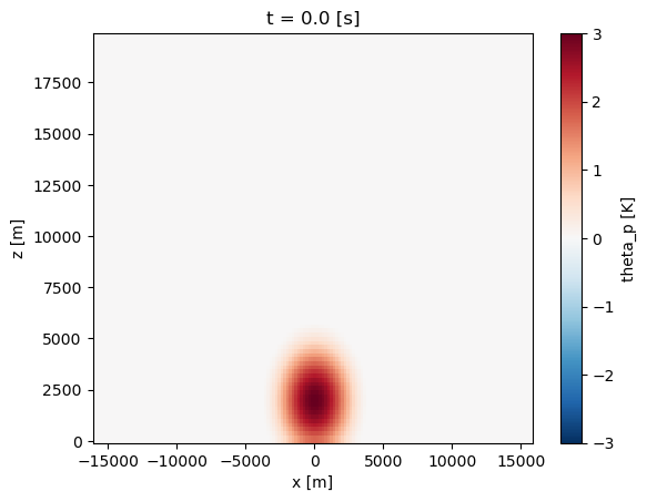
Running the model forward in time
Now, we can actually start integrating in time. At the first timestep, we don’t have the data to use leapfrog integration, so we need a special first timestep that does a forward-in-time approach (also known as Euler forward differencing):
# Integrate the model, saving after desired timestep counts
model.take_first_timestep()
results.append(model.current_state())
TODO: fix/adjust approach later
Now, the model (as written above) has been found to have a numerical instability that causes the model to “explode” within 30 seconds of simulated time. To showcase how such a model can go wrong, we save results every timestep, as follows:
for _ in range(3000):
    model.integrate(1)
    results.append(model.current_state())

# Merge results
ds = xr.concat(results, 't')
ax = results[0]['pi'][0].plot.imshow( cmap='RdBu_r')
# fig = ax.get_figure()
# fig.savefig('crash_left.png', dpi=300, bbox_inches='tight')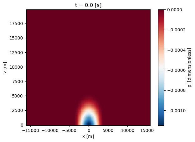
mv = ModelVis(ds)
mv.panespanel_view = cfl_quiver_row(ds, stride=8, cmap='bwr') # or 'jet' if you prefer
panel_view # display in notebook; or panel_view.show(); or panel_vi
Troubleshooting Model Instability
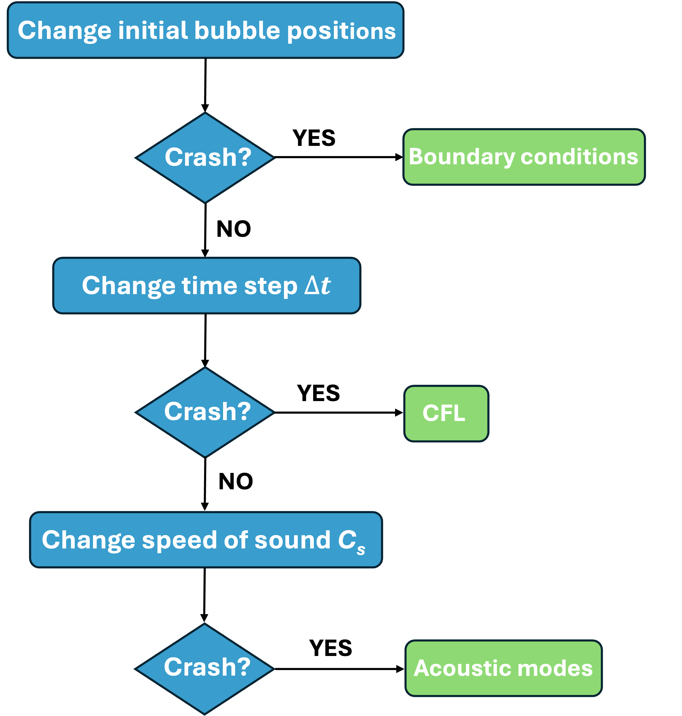
For numerical instability issues (when the model “explodes”), sensitivity testing is a key diagnostic approach. The idea is to identify the variables that may influence stability and then vary them one at a time while keeping all other factors constant. In this case, we present three example tests below:
Change Initial Bubble Position
Purpose: Determine whether instability is caused by inappropriate boundary condition. Procedure:
Place the initial thermal bubble in different positions (center, near top, near bottom, near lateral edges).
Keep all other model parameters fixed. Diagnosis Logic:
If instability occurs only when the bubble is near a specific boundary (e.g., bottom), this points to boundary condition problems such as spurious reflections or incorrect implementation.
model = ModelDriver(
    nx=160, nz=100, dx=200., dz=200., dt=2, c_s_sqr=50.0**2,
    u_tendency=u_tendency, w_tendency=w_tendency, theta_p_tendency=theta_p_tendency, pi_tendency=pi_tendency
)
model.initialize_isentropic_base_state(300., 9.5e4)
#model.initialize_warm_bubble(3.0, 4.0e3, 4.0e3, 0.0e3, 2.0e3)
model.initialize_warm_bubble(3.0, 4.0e3, 4.0e3, 0.0e3, 2.0e3)
# Start saving results
results = []
results.append(model.current_state())
Change Time Step ()
Purpose: Test the temporal stability of the time integration scheme and check CFL compliance. Procedure:
Reduce () incrementally (e.g., 0.01 → 0.005 → 0.001 s).
Run simulations for each Δt without changing spatial resolution or physical parameters.
If instability disappears or is delayed when Δt is reduced, the issue may be CFL condition violation or insufficient temporal resolution for fast modes (acoustic or gravity waves).
If there is no change, instability may not be driven by time step size.
Change Speed of Sound (cs)
Purpose: Isolate the role of acoustic modes in driving instability. Procedure:
Modify Cs in the model physics.
Lower values slow acoustic waves; higher values speed them up.
If stability changes when csc_scs
changes, acoustic wave behavior and their interactions with boundaries are important. This also indirectly modifies the acoustic CFL condition, so link findings back to Test 2 results.
Summary
The preceding cookbook provided a crash-course on the development of a 2-D Mesoscale Numerical Model, starting with the basic dynamical equations through the conversion to computer code and ultimately model integration. This pre-configured “test-case” is intended to be used for educational purposes only. Note that all the assumptions/configurations used herein may not be applicable for other situations. Future notebooks are to be included, demonstrating how various configurations (i.e., equation simplifications, discretization schemes, boundary conditions, grid styles, and spatiotemporal resolutions) all influences the performance and accuracy of the resultant output. Additionally, we plan to include explicit walk-throughs regarding stability analyses, corrections, and filtering techniques. Check-in regularly for updates to this Cookbook.
What’s next?
TODO: reference later portions
Resources
TODO: add these
- Klemp, J. B., & Wilhelmson, R. B. (1978). The simulation of three-dimensional convective storm dynamics. J. Atmos. Sci., 35(6), 1070–1096.
- Harris, C. R., Millman, K. J., van der Walt, S. J., Gommers, R., Virtanen, P., Cournapeau, D., Wieser, E., Taylor, J., Berg, S., Smith, N. J., Kern, R., Picus, M., Hoyer, S., van Kerkwijk, M. H., Brett, M., Haldane, A., del Río, J. F., Wiebe, M., Peterson, P., … Oliphant, T. E. (2020). Array programming with NumPy. Nature, 585(7825), 357–362. 10.1038/s41586-020-2649-2
- Hoyer, S., & Hamman, J. (2017). xarray: N-D labeled Arrays and Datasets in Python. Journal of Open Research Software, 5(1), 10. 10.5334/jors.148