Gill-Matsuno model - Atmos-modeling Cookbook

The Gill-Matsuno model is a classical atmospheric model that describes the tropical atmospheric response to a prescribed heating. It consists of 3 prognostic variables $u$ , $v$ , and $p$ in an equatorial beta-plane approximation. The non-dimensional form of the equations is given by:

\frac{\partial u}{\partial t} + \epsilon u - \frac{1}{2} yv = -\frac{\partial p}{\partial x} \\ \frac{\partial v}{\partial t} + \epsilon v + \frac{1}{2} yu = -\frac{\partial p}{\partial y} \\ \frac{\partial p}{\partial t} + \epsilon p + \frac{\partial u}{\partial x} + \frac{\partial v}{\partial y} = -Q

(1)

This cookbook aims to reproduce the results of the classical Gill-Matsuno model experiment in different forcing scenarios. The model is set up on a grid with prescribed parameters, and the forcing function $Q$ is defined to represent the heating in the atmosphere. Here we will explore the steady-state solution of the set of equations outline above, which is often used to analyze the tropical atmospheric dynamics in a simplified manner.

Imports¶

import time

import holoviews as hv
import hvplot.xarray
import matplotlib.pyplot as plt
import numba
import numpy as np
import xarray as xr

hv.output(widget_location="top")

Discretization¶

The numerical scheme used to solve the equations is a forward-in-time, centered-in-space finite difference method. The steady-state solution of the system will be reached by model convergence after a sufficient number of time steps. Solving for $\partial / \partial t$ , equation (1) becomes:

\frac{\partial u}{\partial t} = -\frac{\partial p}{\partial x} - \epsilon u + \frac{1}{2} yv

(2)

\frac{\partial v}{\partial t} = -\frac{\partial p}{\partial y} - \epsilon v - \frac{1}{2} yu

(3)

\frac{\partial p}{\partial t} = -Q - \epsilon p - ( \frac{\partial u}{\partial x} + \frac{\partial v}{\partial y} )

(4)

We will shift our focus to the terms that need discretization first

Pressure Gradient Force (PGF)¶

The first term on the RHS of (2) and (3) represents the pressure gradient force. The discretization of this term looks as follow:

-\frac{\partial p}{\partial x} \approx -\frac{p^{\tau}_{i+1,j} - p^{\tau}_{i-1,j}}{2\Delta x}

(5)

-\frac{\partial p}{\partial y} \approx -\frac{p^{\tau}_{i,j+1} - p^{\tau}_{i,j-1}}{2\Delta y}

(6)

@numba.njit
def pressure_gradient_x(p, dx):
    """Calculates the pressure gradient in the x-direction."""
    term = np.zeros_like(p)
    for i in range(1, p.shape[0] - 1):
        for j in range(1, p.shape[1] - 1):
            term[i, j] = -(p[i + 1, j] - p[i - 1, j]) / (2 * dx)
    return term


@numba.njit
def pressure_gradient_y(p, dy):
    """Calculates the pressure gradient in the y-direction."""
    term = np.zeros_like(p)
    for i in range(1, p.shape[0] - 1):
        for j in range(1, p.shape[1] - 1):
            term[i, j] = -(p[i, j + 1] - p[i, j - 1]) / (2 * dy)
    return term

Divergence¶

The third term on the RHS of (4) represents the divergence of the velocity field. The discretization of this term looks as follow:

-( \frac{\partial u}{\partial x} + \frac{\partial v}{\partial y} ) \approx -\frac{u^{\tau}_{i+1,j} - u^{\tau}_{i-1,j}}{2\Delta x} - \frac{v^{\tau}_{i,j+1} - v^{\tau}_{i,j-1}}{2\Delta y}

(7)

@numba.njit
def divergence(u, v, dx, dy):
    """Calculates the divergence for the pressure equation."""
    term = np.zeros_like(u)
    for i in range(1, u.shape[0] - 1):
        for j in range(1, u.shape[1] - 1):
            du_dx = (u[i + 1, j] - u[i - 1, j]) / (2 * dx)
            dv_dy = (v[i, j + 1] - v[i, j - 1]) / (2 * dy)
            term[i, j] = -(du_dx + dv_dy)
    return term

Damping¶

The Gill-Matsuno model includes a damping term to account for dissipative processes in the atmosphere. This is given by the $\epsilon$ parameter found as the second term of the RHS of (2), (3), and (4) that does not involve any derivatives.

-\epsilon u \approx -\epsilon u^{\tau}_{i,j} \\ -\epsilon v \approx -\epsilon v^{\tau}_{i,j} \\ -\epsilon p \approx -\epsilon p^{\tau}_{i,j}

(8)

@numba.njit
def damping(field, epsilon):
    """Calculates the damping for a given field."""
    return -epsilon * field

Coriolis¶

In the equatorial beta-plane approximation, the non-dimensional form of the Coriolis term is given by the last term on the RHS of equations (2) and (3). It is represented as follows:

\frac{1}{2} yv = \frac{1}{2} y v^{\tau}_{i,j}

(9)

The expression for (3) is equivalent but with $u$ instead of $v$ and of negative sign.

@numba.njit
def coriolis_term(field, yy, sign=1):
    """Calculates the Coriolis term"""
    return 0.5 * yy * field * sign

Heating¶

The heating rate $Q$ on equation (4) is used to study the heat-induced tropical circulation response on a resting atmosphere. The function create_heating generates a 2D heating field that can be used in the model.

def create_heating(xx, yy):
    """
    Creates a 2D localized, symmetric heating function (Q).
    """
    Q = np.zeros_like(xx)
    L_forcing = 2.0

    # Define a mask for where the heating is active
    heating_mask = (xx > 4 * L_forcing) & (xx < 6 * L_forcing)

    # Calculate the heating within the masked region
    Q[heating_mask] = -(
        np.sin(np.pi / (2 * L_forcing) * xx[heating_mask])
        * np.exp(-0.25 * yy[heating_mask] ** 2)
    )
    da = xr.DataArray(
        Q, dims=("x", "y"), coords={"x": xx[:, 0], "y": yy[0, :]}, name="Q"
    )
    return da

Boundary Conditions¶

Before putting everything together, we need to define the boundary conditions for our system. These conditions will ensure that our model behaves correctly at the edges of the computational domain. Here we implement the periodic boundary conditions in the zonal direction with a zero-gradient meridional boundary condition.

@numba.njit
def apply_boundary_conditions(u, v, p):
    """
    Applies periodic zonal and zero-gradient meridional boundary conditions.
    """
    # Periodic in x (zonal)
    u[0, :], u[-1, :] = u[-2, :], u[1, :]
    v[0, :], v[-1, :] = v[-2, :], v[1, :]
    p[0, :], p[-1, :] = p[-2, :], p[1, :]

    # Zero-gradient in y (meridional)
    u[:, 0], u[:, -1] = u[:, 1], u[:, -2]
    v[:, 0], v[:, -1] = v[:, 1], v[:, -2]
    p[:, 0], p[:, -1] = p[:, 1], p[:, -2]

    return u, v, p

Tendency¶

Now that we have defined all the RHS terms, we can express the time tendency terms for the set of equations (2), (3), and (4) in a forward scheme as follows:

u^{\tau+1} = u^\tau + \Delta t \frac{\partial u}{\partial t} \\ v^{\tau+1} = v^\tau + \Delta t \frac{\partial v}{\partial t} \\ p^{\tau+1} = p^\tau + \Delta t \frac{\partial p}{\partial t}

(10)

Which relates the next time step to the current state of the system. The time derivatives in this equation have already been discretized and can be expressed as follow

\frac{\partial u}{\partial t} = PGF + Damping + Coriolis \\ \frac{\partial v}{\partial t} = PGF + Damping + Coriolis \\ \frac{\partial p}{\partial t} = Heating + Damping + Divergence

(11)

The solver loop takes all of the above equations and iteratively updates the state of the system at each time step. This process continues until the desired simulation time is reached.

@numba.njit
def numba_solver_loop(u, v, p, Q, yy, params_tuple):
    """
    Performs the time-stepping
    """
    # Unpack parameters
    dt, dx, dy, eps_u, eps_v, eps_p, num_steps = params_tuple

    # Time-stepping loop
    for tau in range(num_steps - 1):
        # Get the current state (a 2D slice)
        u_tau, v_tau, p_tau = u[tau, :, :], v[tau, :, :], p[tau, :, :]

        # Calculate full tendency fields using the current state
        du_dt = (
            damping(u_tau, eps_u)
            + coriolis_term(v_tau, yy, 1)
            + pressure_gradient_x(p_tau, dx)
        )
        dv_dt = (
            damping(v_tau, eps_v)
            + coriolis_term(u_tau, yy, -1)
            + pressure_gradient_y(p_tau, dy)
        )
        dp_dt = damping(p_tau, eps_p) + divergence(u_tau, v_tau, dx, dy) + Q

        # Update the NEXT time slice in the main arrays
        u[tau + 1, :, :] = u_tau + du_dt * dt
        v[tau + 1, :, :] = v_tau + dv_dt * dt
        p[tau + 1, :, :] = p_tau + dp_dt * dt

        # Apply Boundary Conditions
        u[tau + 1, :, :], v[tau + 1, :, :], p[tau + 1, :, :] = (
            apply_boundary_conditions(
                u[tau + 1, :, :], v[tau + 1, :, :], p[tau + 1, :, :]
            )
        )

Model Setup¶

Now that we have taken care of the equations, all we have left is to set up the model by defining the grid, initial conditions, and parameters. This will provide the foundation for our numerical simulations. For this implementation, we have the following parameters

$L_x$ : Length of the domain in the x direction. 1 unit here translates to 10 degrees of latitude/longitude.
$L_y$ : Half-length of the domain in the y direction. A value of 5 corresponds to a domain from -5 to 5.
$dx$ : Grid spacing in the x direction.
$dy$ : Grid spacing in the y direction.
$dt$ : Time step size.
$eps_u$ , $eps_v$ , $eps_p$ : Damping coefficients for the u, v, and p fields, respectively.
$num_steps$ : Number of time steps to simulate.

model_parameters = {
    "Lx": 25.0,
    "Ly": 5.0,
    "dx": 0.5,
    "dy": 0.5,
    "dt": 0.02,
    "eps_u": 0.1,
    "eps_v": 0.1,
    "eps_p": 0.1,
    "num_steps": 3000,
}

Using these parameters, we can create the grid and include that inside our model_parameters dictionary.

def create_grid(params):
    """Creates the computational grid based on the provided parameters."""
    Lx, Ly, dx, dy = params["Lx"], params["Ly"], params["dx"], params["dy"]
    xs = np.arange(0, Lx + dx, dx)
    ys = np.arange(-Ly, Ly + dy, dy)
    xx, yy = np.meshgrid(xs, ys, indexing="ij")
    return {"xs": xs, "ys": ys, "xx": xx, "yy": yy}

model_parameters["grid"] = create_grid(model_parameters)

The heating can be created now that we have the grid information.

model_parameters["Q"] = create_heating(
    model_parameters["grid"]["xx"], model_parameters["grid"]["yy"]
)
model_parameters["Q"].plot(cmap="Reds_r", x="x", figsize=(12.5, 5), add_colorbar=False)
plt.title("Heating $Q$")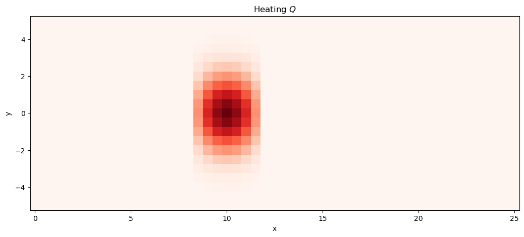

If you want to define your own model parameters, remember to call the functions like this

model_parameters = {
    'Lx': 25.0, 'Ly': 5.0,
    'dx': 0.5, 'dy': 0.5,
    'dt': 0.01,
    'eps_u': 0.1, 'eps_v': 0.1, 'eps_p': 0.1,
    'num_steps': 3000,
}
model_parameters["grid"] = create_grid(model_parameters)
model_parameters["Q"] = create_heating(model_parameters["grid"]['xx'], model_parameters["grid"]['yy'])

Running the model¶

Now we are ready to run the model. The next function will take care of building the grid, initializing the arrays and creating the heating that goes into the simulation.

def setup_and_run_model(params):
    """Sets up the grid and initial conditions, then runs the solver."""
    num_steps = params["num_steps"]
    grid = params["grid"]

    x_dim, y_dim = len(grid["xs"]), len(grid["ys"])

    # Create 3D arrays with time as the first dimension
    u = np.zeros((num_steps, x_dim, y_dim))
    v = np.zeros_like(u)
    p = np.zeros_like(u)

    # Pack parameters for Numba
    params_tuple = (
        params["dt"],
        params["dx"],
        params["dy"],
        params["eps_u"],
        params["eps_v"],
        params["eps_p"],
        num_steps,
    )

    print("🚀 Starting simulation...")
    start_time = time.time()

    # Run the solver (we extract data from Q to convert it from xarray -> numpy)
    numba_solver_loop(u, v, p, params["Q"].data, grid["yy"], params_tuple)

    end_time = time.time()
    print(f"✅ Simulation finished in {end_time - start_time:.2f} seconds.")

    ds = xr.Dataset(
        {
            "u": xr.DataArray(
                u,
                dims=("time", "x", "y"),
                coords={
                    "time": np.arange(u.shape[0]),
                    "x": grid["xs"],
                    "y": grid["ys"],
                },
            ),
            "v": xr.DataArray(
                v,
                dims=("time", "x", "y"),
                coords={
                    "time": np.arange(v.shape[0]),
                    "x": grid["xs"],
                    "y": grid["ys"],
                },
            ),
            "p": xr.DataArray(
                p,
                dims=("time", "x", "y"),
                coords={
                    "time": np.arange(p.shape[0]),
                    "x": grid["xs"],
                    "y": grid["ys"],
                },
            ),
        }
    )

    return ds

The first time we run the model it will take longer so numba will compile the functions. Subsequent calls will be faster.

model_output = setup_and_run_model(model_parameters)

🚀 Starting simulation...

✅ Simulation finished in 9.49 seconds.

Visualize the results¶

Since we are wrapping the results using xarray, we can take advantage of its powerful visualization capabilities.

plot_kwargs = dict(x="x", add_colorbar=False)
fig, ax = plt.subplots(figsize=(12.5, 5))
model_output["p"].isel(time=-1).plot.contourf(ax=ax, cmap="Blues_r", **plot_kwargs)
model_output["p"].isel(time=-1).plot.contour(
    ax=ax, colors="k", linewidths=0.5, **plot_kwargs
)
model_output.isel(time=-1).thin(x=3, y=2).plot.quiver(
    ax=ax, x="x", y="y", u="u", v="v", scale=30, color="k", width=0.003, add_guide=False
)
ax.set_title("Gill-Matsuno output from symmetric forcing")
ax.set_xlabel("Zonal Distance (x)")
ax.set_ylabel("Meridional Distance (y)")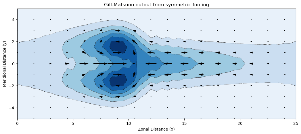

We can visualize the individual time steps interactively by using hvplot.

The quiver plot is called vectorfield in hvplot and it requires magnitude and angle instead of u and v components.

# We reduce the number of frames this way
model_output_hv = model_output.thin(time=100)
model_output_hv["time"] = np.arange(model_output_hv.u.shape[0])
mag = np.sqrt(model_output_hv.u**2 + model_output_hv.v**2)
angle = (np.pi / 2.0) - np.arctan2(model_output_hv.u / mag, model_output_hv.v / mag)

ds = xr.Dataset(
    {
        "mag": xr.DataArray(
            mag,
            dims=("time", "x", "y"),
            coords={
                "y": model_parameters["grid"]["ys"],
                "x": model_parameters["grid"]["xs"],
                "time": np.arange(mag.shape[0]),
            },
        ),
        "angle": xr.DataArray(
            angle,
            dims=("time", "x", "y"),
            coords={
                "y": model_parameters["grid"]["ys"],
                "x": model_parameters["grid"]["xs"],
                "time": np.arange(angle.shape[0]),
            },
        ),
    }
)

Now we can create the interactive plot

levels = np.arange(-2, 0.5, 0.2)
plot_ops = dict(
    groupby="time",
    x="x",
    y="y",
    hover=False,
    colorbar=False,
    legend=False,
    dynamic=False,
)
over = (
    model_output_hv.p.hvplot.contourf(levels=levels, cmap="Blues_r", **plot_ops)
    * model_output_hv.p.hvplot.contour(
        levels=levels, cmap=["black"] * len(levels), **plot_ops
    )
    * ds.hvplot.vectorfield(angle="angle", mag="mag", **plot_ops).opts(magnitude="mag")
)
over

Introduction

Introductory Concepts in Atmospheric Modeling

Introduction

Crash Course Towards Your First Model