Overview
This notebook shows an advanced analysis case. The calculation was inspired by Angie Pendergrass’s work on precipitation statistics, as described in the following websites / papers:
We use xhistogram to calculate the distribution of precipitation intensity and its changes in a warming climate.
Prerequisites
| Concepts | Importance | Notes |
|---|---|---|
| Intro to Xarray | Necessary | |
| Understanding of NetCDF | Helpful | Familiarity with metadata structure |
| Dask | Helpful |
Time to learn: 5 minutes
Imports
import os
import sys
from matplotlib import pyplot as plt
import numpy as np
import pandas as pd
import xarray as xr
import fsspec
from tqdm.autonotebook import tqdm
from xhistogram.xarray import histogram
from dask_gateway import Gateway
from dask.distributed import Client

%matplotlib inline
plt.rcParams['figure.figsize'] = 12, 6
/tmp/ipykernel_4147/106887996.py:8: TqdmExperimentalWarning: Using `tqdm.autonotebook.tqdm` in notebook mode. Use `tqdm.tqdm` instead to force console mode (e.g. in jupyter console)
from tqdm.autonotebook import tqdm
Compute Cluster
Here we use a dask cluster to parallelize our analysis.
platform = sys.platform

if (platform == 'win32'):
    import multiprocessing.popen_spawn_win32
else:
    import multiprocessing.popen_spawn_posix
Initiate the Dask client:
client = Client()
client
Loading...
Load Data Catalog
df = pd.read_csv('https://storage.googleapis.com/cmip6/cmip6-zarr-consolidated-stores.csv')
df.head()
Loading...
df_3hr_pr = df[(df.table_id == '3hr') & (df.variable_id == 'pr')]
len(df_3hr_pr)78run_counts = df_3hr_pr.groupby(['source_id', 'experiment_id'])['zstore'].count()
run_countssource_id experiment_id
BCC-CSM2-MR historical 1
ssp126 1
ssp245 1
ssp370 1
ssp585 1
CNRM-CM6-1 highresSST-present 1
historical 3
ssp126 1
ssp245 1
ssp370 1
ssp585 1
CNRM-CM6-1-HR highresSST-present 1
CNRM-ESM2-1 historical 1
ssp126 1
ssp245 1
ssp370 1
ssp585 1
GFDL-CM4 1pctCO2 2
abrupt-4xCO2 2
amip 2
historical 2
piControl 2
GFDL-CM4C192 highresSST-future 1
highresSST-present 1
GFDL-ESM4 1pctCO2 1
abrupt-4xCO2 1
esm-hist 1
historical 1
ssp119 1
ssp126 1
ssp370 1
GISS-E2-1-G historical 2
HadGEM3-GC31-HM highresSST-present 1
HadGEM3-GC31-LM highresSST-present 1
HadGEM3-GC31-MM highresSST-present 1
IPSL-CM6A-ATM-HR highresSST-present 1
IPSL-CM6A-LR highresSST-present 1
historical 15
piControl 1
ssp126 3
ssp245 2
ssp370 10
ssp585 1
MRI-ESM2-0 historical 1
Name: zstore, dtype: int64source_ids = []
experiment_ids = ['historical', 'ssp585']
for name, group in df_3hr_pr.groupby('source_id'):
if all([expt in group.experiment_id.values
for expt in experiment_ids]):
source_ids.append(name)
source_ids
# Use only one model. Otherwise it takes too long to run on GitHub.
source_ids = ['BCC-CSM2-MR']def load_pr_data(source_id, expt_id):
"""
Load 3hr precip data for given source and expt ids
"""
uri = df_3hr_pr[(df_3hr_pr.source_id == source_id) &
(df_3hr_pr.experiment_id == expt_id)].zstore.values[0]
ds = xr.open_zarr(fsspec.get_mapper(uri), consolidated=True)
return dsdef precip_hist(ds, nbins=100, pr_log_min=-3, pr_log_max=2):
"""
Calculate precipitation histogram for a single model.
Lazy.
"""
assert ds.pr.units == 'kg m-2 s-1'
# mm/day
bins_mm_day = np.hstack([[0], np.logspace(pr_log_min, pr_log_max, nbins)])
bins_kg_m2s = bins_mm_day / (24*60*60)
pr_hist = histogram(ds.pr, bins=[bins_kg_m2s], dim=['lon']).mean(dim='time')
log_bin_spacing = np.diff(np.log(bins_kg_m2s[1:3])).item()
pr_hist_norm = 100 * pr_hist / ds.dims['lon'] / log_bin_spacing
pr_hist_norm.attrs.update({'long_name': 'zonal mean rain frequency',
'units': '%/Δln(r)'})
return pr_hist_norm
def precip_hist_for_expts(dsets, experiment_ids):
"""
Calculate histogram for a suite of experiments.
Eager.
"""
# actual data loading and computations happen in this next line
pr_hists = [precip_hist(ds).load()
for ds in [ds_hist, ds_ssp]]
pr_hist = xr.concat(pr_hists, dim=xr.Variable('experiment_id', experiment_ids))
return pr_histresults = {}
for source_id in tqdm(source_ids):
# get a 20 year period
ds_hist = load_pr_data(source_id, 'historical').sel(time=slice('1980', '2000'))
ds_ssp = load_pr_data(source_id, 'ssp585').sel(time=slice('2080', '2100'))
pr_hist = precip_hist_for_expts([ds_hist, ds_ssp], experiment_ids)
results[source_id] = pr_histLoading...
def plot_precip_changes(pr_hist, vmax=5):
    """
    Visualize the output
    """
    pr_hist_diff = (pr_hist.sel(experiment_id='ssp585') -
                    pr_hist.sel(experiment_id='historical'))
    pr_hist.sel(experiment_id='historical')[:, 1:].plot.contour(xscale='log', colors='0.5', levels=21)
    pr_hist_diff[:, 1:].plot.contourf(xscale='log', vmax=vmax, levels=21)
title = 'Change in Zonal Mean Rain Frequency'
for source_id, pr_hist in results.items():
plt.figure()
plot_precip_changes(pr_hist)
plt.title(f'{title}: {source_id}')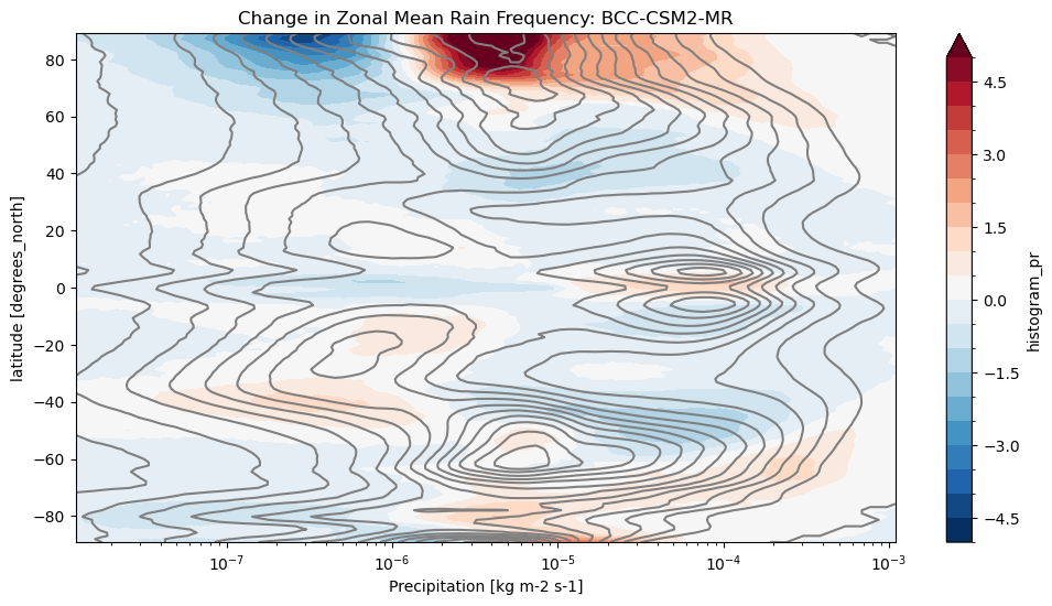
We’re at the end of the notebook, so let’s shutdown our Dask cluster.
client.shutdown()Summary
In this notebook, we used CMIP6 data to compare precipitation intensity in the SSP585 scenario to historical runs.
What’s next?
More examples of using CMIP6 data.
Resources and references
Original notebook in the Pangeo Gallery by Henri Drake and Ryan Abernathey
- Pendergrass, A. G., & Deser, C. (2017). Climatological Characteristics of Typical Daily Precipitation. Journal of Climate, 30(15), 5985–6003. 10.1175/jcli-d-16-0684.1