Scipy - Feature Tracking Cookbook

Overview¶

In this notebook, you will learn how to develop and implement your own algorithm that detects and tracks different precipitation features throughout a 12-hour period using ERA5 data using Scipy’s label function. Although this notebook focuses on precipitation by using QPF, this can easily be applied to other variables that don’t require pre-processing. By the end of this notebook, you should be able to/understand:

How Scipy’s label function works, including how feature merges/break-ups are handled.
How to identify different features using Scipy’s label function, and why a minimum precipitation threshold is needed.
Why using Scipy’s detection algorithm across multiple time steps is insufficient for feature tracking.
How to implement a tracking algorithm that tracks how precipitation features move throughout the time period.
Limitations to using the feature tracking algorithm, including understanding the distribution of the length of different precipitation features.

Let’s get started!

Prerequisites¶

Concepts	Importance	Notes
xarray	Necessary
matplotlib	Necessary
Cartopy	Necessary	Needed to plot geospatial data
scipy-image	Useful	Useful reference for Scipy’s label function
IPython	Useful	For inline animation

Time to learn: 30-45 minutes

Import Packages¶

import xarray as xr
from scipy.ndimage import label, generate_binary_structure
import matplotlib.pyplot as plt
import cartopy.crs as ccrs
import cartopy.feature as cfeature
import numpy as np
from matplotlib.animation import FuncAnimation
from IPython.display import HTML

import matplotlib.colors as mcolors
from matplotlib.cm import ScalarMappable
import pandas as pd
import math

Scipy Precipitation Feature Detection Algorithm¶

Let’s go through the basic steps to identify each precipitation feature.¶

Open the dataset using xarray

data = xr.open_dataset('data/precip_ex.nc')

Select a time to specifically do the subset of the data

time = data.time[0]
subset_data = data.sel(time=time)

In order to account for individual features, anywhere less than 0.25mm/hr of precip will be set to zero. This is so that areas of minimal/weak precipitation are not grouped with zero to create a single mega precipitation field over the entire Earth.

no_minimal_precip = subset_data['ETC_tp'].where(subset_data['ETC_tp'] > 0.25, 0)
s = generate_binary_structure(2,2)

Run through labeling feature algorithm

labeled_data, num_data = label(no_minimal_precip, structure=s)

Let’s look at all of the data plotted first.¶

plt.figure(figsize=(15,8))
ax = plt.axes(projection=ccrs.PlateCarree())

## Create two-dimensional grid for latitude and longitude
lon2d, lat2d = np.meshgrid(no_minimal_precip['longitude'], no_minimal_precip['latitude'])

plt.contourf(lon2d, lat2d, labeled_data, cmap='tab20', transform=ccrs.PlateCarree())

ax.add_feature(cfeature.LAND)
ax.add_feature(cfeature.BORDERS, edgecolor='black')
ax.add_feature(cfeature.STATES, edgecolor='black')

ax.add_feature(cfeature.COASTLINE, edgecolor='black')

provinces = cfeature.NaturalEarthFeature(
    category='cultural',
    name='admin_1_states_provinces_lines',
    scale='50m',
    facecolor='none',
    edgecolor='black'
)
ax.add_feature(provinces)
ax.gridlines(draw_labels=True)

<cartopy.mpl.gridliner.Gridliner at 0x7f09b45296a0>

/home/runner/micromamba/envs/feature-tracking-dev/lib/python3.14/site-packages/cartopy/io/__init__.py:242: DownloadWarning: Downloading: https://naturalearth.s3.amazonaws.com/110m_physical/ne_110m_land.zip
  warnings.warn(f'Downloading: {url}', DownloadWarning)

/home/runner/micromamba/envs/feature-tracking-dev/lib/python3.14/site-packages/cartopy/io/__init__.py:242: DownloadWarning: Downloading: https://naturalearth.s3.amazonaws.com/110m_cultural/ne_110m_admin_0_boundary_lines_land.zip
  warnings.warn(f'Downloading: {url}', DownloadWarning)

/home/runner/micromamba/envs/feature-tracking-dev/lib/python3.14/site-packages/cartopy/io/__init__.py:242: DownloadWarning: Downloading: https://naturalearth.s3.amazonaws.com/110m_cultural/ne_110m_admin_1_states_provinces_lakes.zip
  warnings.warn(f'Downloading: {url}', DownloadWarning)

/home/runner/micromamba/envs/feature-tracking-dev/lib/python3.14/site-packages/cartopy/io/__init__.py:242: DownloadWarning: Downloading: https://naturalearth.s3.amazonaws.com/50m_cultural/ne_50m_admin_1_states_provinces_lines.zip
  warnings.warn(f'Downloading: {url}', DownloadWarning)

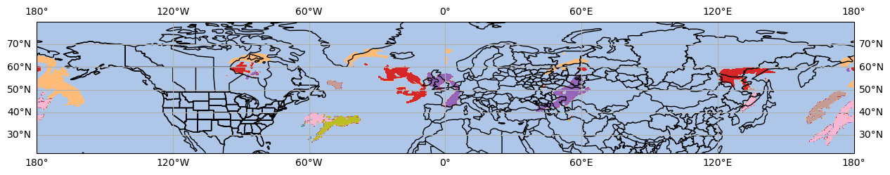
Woah! This is neat! But how does this algorithm truly work? To understand this, let’s focus on one particular precipitation event.

Understanding the Algorithm: Plotting One Specific Feature Through Time¶

The precip_time_index function pulls out the subset of the data that is specific to a partiuclar time.

def precip_time_index(full_data, time_index):
    time = full_data.time[time_index]
    subset_data = full_data.sel(time=time)

    return subset_data

The precip_feature function performs the detection algorithm we set out above. This includes selecting a time index to subset the data and perform the detection on.

def precip_feature(data, time_index):
    subset_data = precip_time_index(data, time_index)

    no_minimal_precip = subset_data['ETC_tp'].where(subset_data['ETC_tp'] > 0.25, 0)
    s = generate_binary_structure(2,2)

    labeled_data, num_data = label(no_minimal_precip, structure=s)

    return labeled_data

Since we are interested in only plotting one specific feature, let’s pick out the feature that is assigned label = 1 through the subset_precip_feature function.

def subset_precip_feature(full_data):
    return np.where(full_data, full_data==1, 0)

Let’s go ahead and plot this one specific feature throughout the full 12 hours of the event.

for i in range(len(data['time'])):
    plt.figure(figsize=(15,8))
    ax = plt.axes(projection=ccrs.PlateCarree())
    lon2d, lat2d = np.meshgrid(no_minimal_precip['longitude'], no_minimal_precip['latitude'])
    subset_labeled_data = subset_precip_feature(precip_feature(data, i))
    plt.contour(lon2d, lat2d, subset_labeled_data, cmap='tab20b', transform=ccrs.PlateCarree())
    precip_data = precip_time_index(data, i)['ETC_tp'].to_numpy()
    precip_data[precip_data <= 0] = np.nan
    im = plt.pcolormesh(lon2d, lat2d, precip_data, cmap='BrBG', transform=ccrs.PlateCarree(), vmin=0, vmax=1)

    plt.colorbar(im, label='Precipitation Rate [mm/hr]', shrink=0.4)

    ax.set_extent([60, 150, 70, 80])

    ax.add_feature(cfeature.LAND)
    ax.add_feature(cfeature.BORDERS, edgecolor='black')
    ax.add_feature(cfeature.STATES, edgecolor='black')
    
    ax.add_feature(cfeature.COASTLINE, edgecolor='black')

    plt.title('Precip Feature 1 at Time Index ' + str(i))
    
    provinces = cfeature.NaturalEarthFeature(
        category='cultural',
        name='admin_1_states_provinces_lines',
        scale='50m',
        facecolor='none',
        edgecolor='black'
    )
    ax.add_feature(provinces)
    ax.gridlines(draw_labels=True)

/home/runner/micromamba/envs/feature-tracking-dev/lib/python3.14/site-packages/cartopy/io/__init__.py:242: DownloadWarning: Downloading: https://naturalearth.s3.amazonaws.com/10m_physical/ne_10m_land.zip
  warnings.warn(f'Downloading: {url}', DownloadWarning)

/home/runner/micromamba/envs/feature-tracking-dev/lib/python3.14/site-packages/cartopy/io/__init__.py:242: DownloadWarning: Downloading: https://naturalearth.s3.amazonaws.com/10m_cultural/ne_10m_admin_0_boundary_lines_land.zip
  warnings.warn(f'Downloading: {url}', DownloadWarning)

/home/runner/micromamba/envs/feature-tracking-dev/lib/python3.14/site-packages/cartopy/io/__init__.py:242: DownloadWarning: Downloading: https://naturalearth.s3.amazonaws.com/10m_cultural/ne_10m_admin_1_states_provinces_lakes.zip
  warnings.warn(f'Downloading: {url}', DownloadWarning)

/home/runner/micromamba/envs/feature-tracking-dev/lib/python3.14/site-packages/cartopy/io/__init__.py:242: DownloadWarning: Downloading: https://naturalearth.s3.amazonaws.com/10m_physical/ne_10m_coastline.zip
  warnings.warn(f'Downloading: {url}', DownloadWarning)

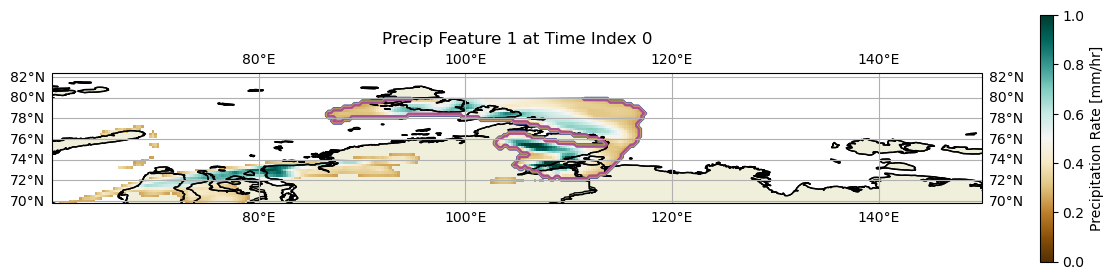
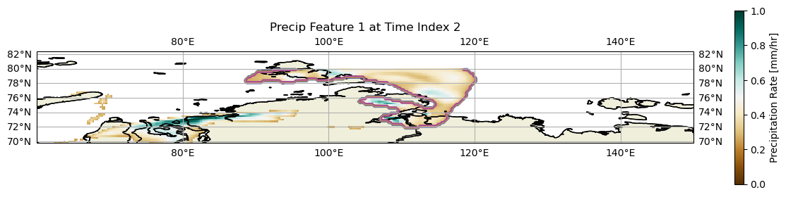
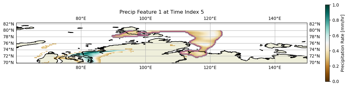
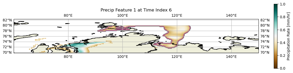
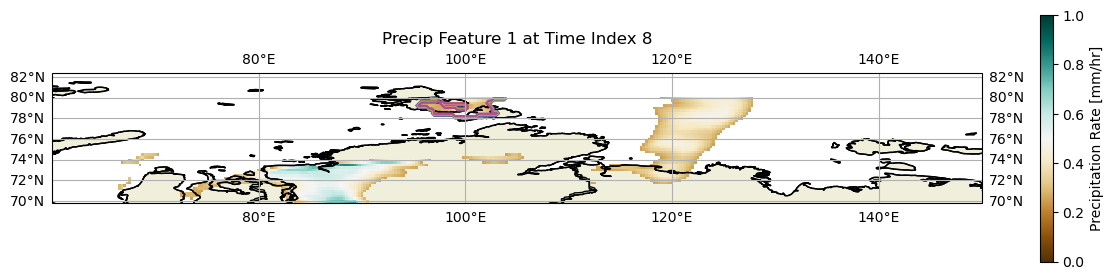
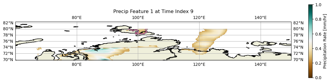
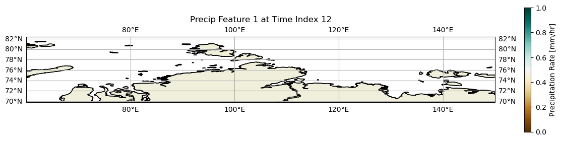
These plots show the identification of a single precipitation feature over time (in contours). The filled contours are the hourly precipitation rate. The dark brown areas throughout each map represent the areas where no precipitation was recorded. Therefore, each area that isn’t a dark dark brown represents a location that received some precipitation.

At time index 0, we can see that feature one corresponds to a large area of precipitation between 95°E and 115°E, as made out by the purple contour. As this area is continuously above 0.25mm/hr, the entire area is assigned to a single feature. With increasing time, the feature can be seen moving eastward, eventually reaching 125°E at time index 6.

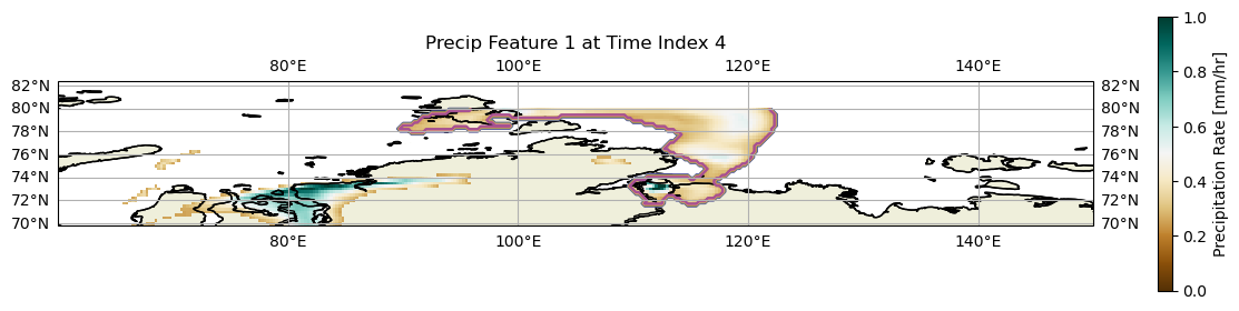
However, at time index 7, the contourseparate no longer corresponds to the area of precipitation centered over 120°E. Instead, the feature is centered around 100°E. Between time index 6 and 7, these two precipitation areas break apart. Between these two precipitation features, there is now an area with a precipitation rate of less than 0.25mm/hr, the critical rate we set to determine whether it is precipitating. Since these two features can no longer be connected, they are now treated as seperate features. Therefore, the purple contour is located only over the precipitation feature at 100°E and not 120°E.

Between time indices 7-that 9, we can observe the precipitation feature continuously shrinks, eventually reaching zero precipitation at time index 10. Since there are no precipitation features within this area, the index assigned to feature 1 is now shifted to a different location and is no longer associated with the feature over northern Siberia.

Creating an animation of the single precipiation feature evolution throughout time.¶

Let’s create an animation of the evolution of this single precipitation feature throughout time.

## Let's create a function to write the figures necessary for the animation.

## Creating a colorbar across all frames.
vmin = 0
vmax = 1
levels = np.linspace(vmin, vmax, 10)
norm = mcolors.Normalize(vmin=vmin, vmax=vmax)
cmap='BrBG'

fig, ax = plt.subplots(subplot_kw={"projection": ccrs.PlateCarree()})

sm = ScalarMappable(norm=norm, cmap=cmap)
sm.set_array([])
cbar = fig.colorbar(sm, ax=ax, pad=0.02, shrink=0.4)
cbar.set_label("Precipitation Rate [mm/hr]")

def func(i):
    ax.clear()
    lon2d, lat2d = np.meshgrid(no_minimal_precip['longitude'], no_minimal_precip['latitude'])
    subset_labeled_data = subset_precip_feature(precip_feature(data, i))
    plt.contour(lon2d, lat2d, subset_labeled_data, cmap='tab20b', transform=ccrs.PlateCarree())
    precip_data = precip_time_index(data, i)['ETC_tp'].to_numpy()
    precip_data[precip_data <= 0] = np.nan
    im = plt.pcolormesh(lon2d, lat2d, precip_data, cmap='BrBG', transform=ccrs.PlateCarree(), vmin=0, vmax=1)

    ax.set_extent([60, 150, 70, 80])

    ax.add_feature(cfeature.LAND)
    ax.add_feature(cfeature.BORDERS, edgecolor='black')
    ax.add_feature(cfeature.STATES, edgecolor='black')
    
    ax.add_feature(cfeature.COASTLINE, edgecolor='black')

    ax.set_title('Precip Feature 1 at Time Index ' + str(i))
    
    provinces = cfeature.NaturalEarthFeature(
        category='cultural',
        name='admin_1_states_provinces_lines',
        scale='50m',
        facecolor='none',
        edgecolor='black'
    )
    ax.add_feature(provinces)
    ax.gridlines(draw_labels=True)
    return fig,


anim = FuncAnimation(fig, func, frames=len(data['time']), interval=300, blit=False)
HTML(anim.to_jshtml())
# anim.save('my_animation.gif', writer='pillow', fps=2)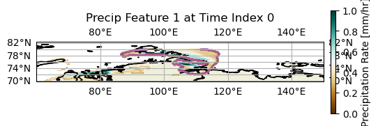

This shows the exact same information as before, just in a nice easy to visualize animation.

Apply this method to worldwide cases.¶

Now that we know how the algorithm works, let’s apply this to all labels worldwide!

for i in range(len(data['time'])):
    plt.figure(figsize=(15,8))
    ax = plt.axes(projection=ccrs.PlateCarree())
    lon2d, lat2d = np.meshgrid(no_minimal_precip['longitude'], no_minimal_precip['latitude'])
    labeled_data = precip_feature(data, i)
    plt.contour(lon2d, lat2d, labeled_data, cmap='tab20b', transform=ccrs.PlateCarree())
    precip_data = precip_time_index(data, i)['ETC_tp'].to_numpy()
    precip_data[precip_data <= 0] = np.nan
    im = plt.pcolormesh(lon2d, lat2d, precip_data, cmap='BrBG', transform=ccrs.PlateCarree(), vmin=0, vmax=1)

    plt.colorbar(im, label='Precipitation Rate [mm/hr]', shrink=0.4)

    ax.add_feature(cfeature.LAND)
    ax.add_feature(cfeature.BORDERS, edgecolor='black')
    ax.add_feature(cfeature.STATES, edgecolor='black')
    
    ax.add_feature(cfeature.COASTLINE, edgecolor='black')

    plt.title('Precip Features at Time Index ' + str(i))
    
    provinces = cfeature.NaturalEarthFeature(
        category='cultural',
        name='admin_1_states_provinces_lines',
        scale='50m',
        facecolor='none',
        edgecolor='black'
    )
    ax.add_feature(provinces)
    ax.gridlines(draw_labels=True)
    plt.tight_layout()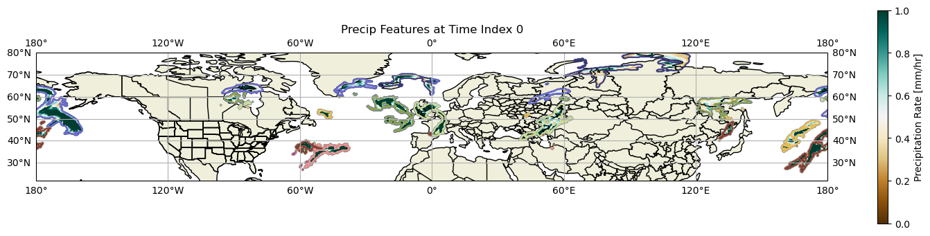

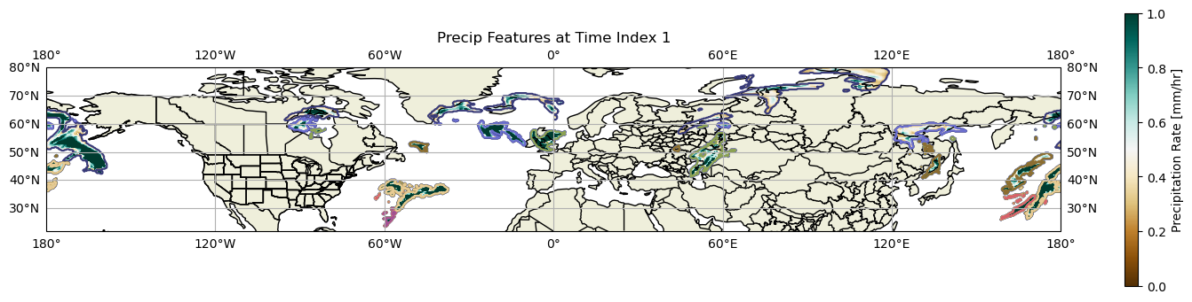
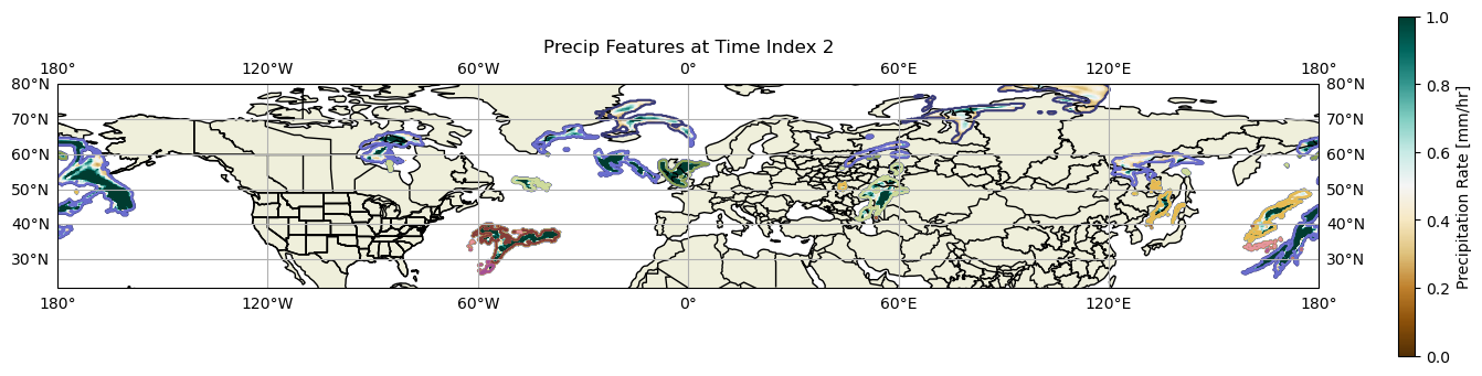
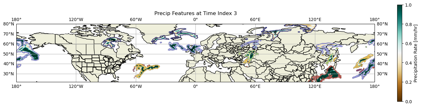
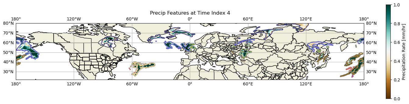
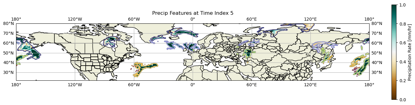
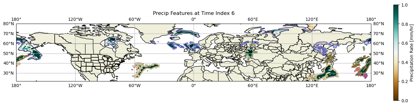
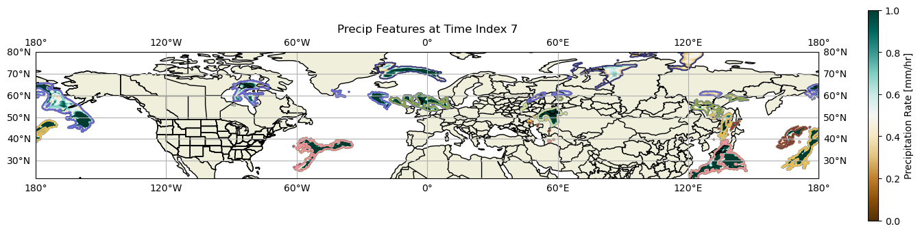
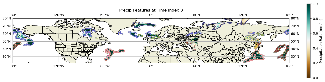
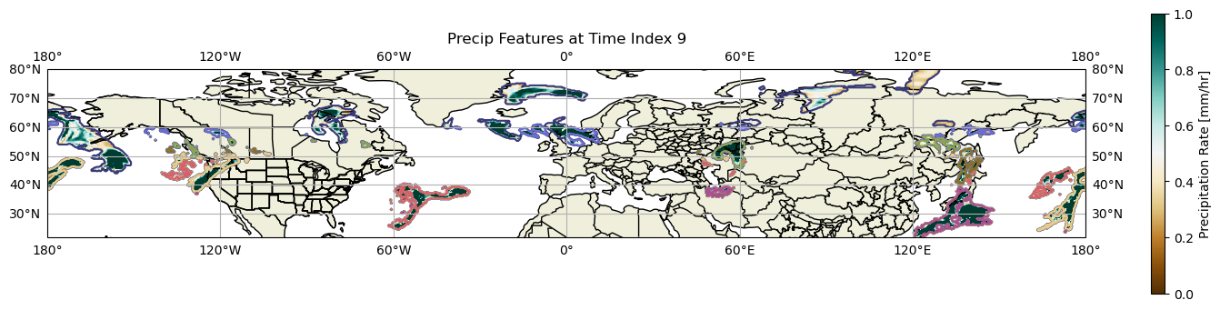
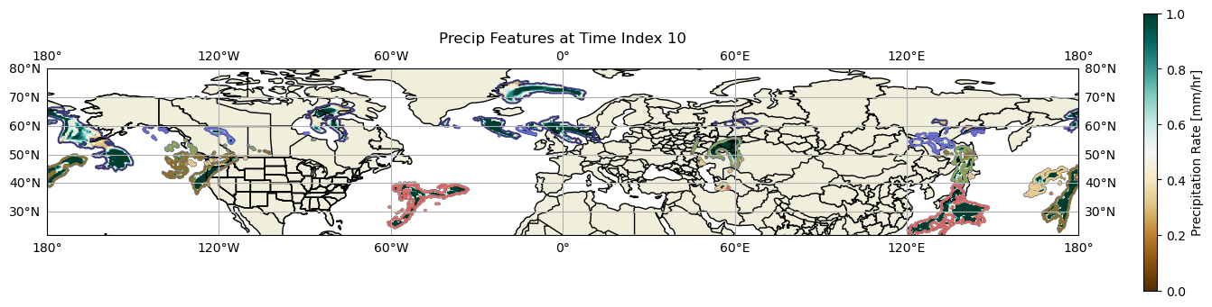
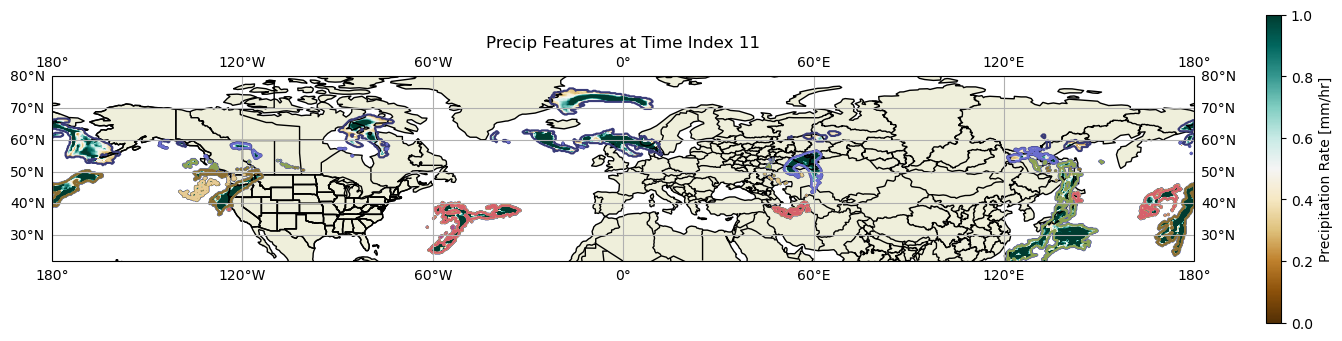
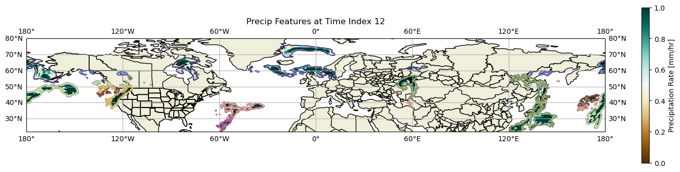
Ok, so we can’t really see much from this diagram, since there’s a lot of contouring going on... Instead of conturing based upon label number, let’s contour based upon the maximum precipitation rate found within the contoured region.

Working with Maximum Precipitation Rate Found within Contoured Region¶

Create an empty array to hold the maximum precipitation rate.

max_precip_rate = np.empty(0)

Get data for time index 0.

lon2d, lat2d = np.meshgrid(no_minimal_precip['longitude'], no_minimal_precip['latitude'])
labeled_data = precip_feature(data, 0)

Get the total number of features within the dataset.

num_features = labeled_data.max()

Go through each feature to determine the maximum precipitation rate within each feature.

## Create a copy of labeled dataset.
new_labeled_data = labeled_data.astype(np.float64)
for i in range(1, num_features+1):
    max_precip_rate = np.append(max_precip_rate, precip_time_index(data, 0)['ETC_tp'].to_numpy()[labeled_data == i].max())
    ## In labeled data, assign every value within labeled_data to max_precip rate assigned. 
    new_labeled_data[new_labeled_data == i] = max_precip_rate[-1]

Now let’s plot this for this specific time!

plt.figure(figsize=(15,8))
ax = plt.axes(projection=ccrs.PlateCarree())
new_labeled_data[new_labeled_data == 0] = np.nan
lon2d, lat2d = np.meshgrid(no_minimal_precip['longitude'], no_minimal_precip['latitude'])
im = plt.contourf(lon2d, lat2d, new_labeled_data, cmap='BrBG', transform=ccrs.PlateCarree(), vmin=0, vmax=10)

plt.colorbar(im, label='Maximum Precipitation Rate [mm/hr]', shrink=0.5)

plt.title('Maximum Precipitation Rate for Each Feature at Time Index 0')

ax.add_feature(cfeature.LAND)
ax.add_feature(cfeature.BORDERS, edgecolor='black')
ax.add_feature(cfeature.STATES, edgecolor='black')
ax.add_feature(cfeature.COASTLINE, edgecolor='black')

ax.gridlines(draw_labels=True)

plt.tight_layout()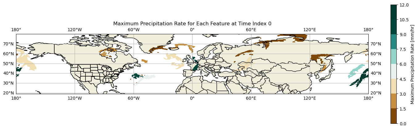

We can now see the maximum precipitation rate found within each precipitation feature at a specific time index! Unsuprisingly, locations in northern latitudes have lower maximum precipitation rates than further south due to the colder air found at these latitudes.

Before we create an animation throughout all time series, let’s create a function get_max_precip_data defining the above process of determining the maximum precipitation rate for each feature found within the time index.

def get_max_precip_data(data, time_index):
    max_precip_rate = np.empty(0)
    labeled_data = precip_feature(data, time_index)
    num_features = labeled_data.max()
    ## Create a copy of labeled dataset.
    new_labeled_data = labeled_data.astype(np.float64)
    for i in range(1, num_features+1):
        max_precip_rate = np.append(max_precip_rate, precip_time_index(data, time_index)['ETC_tp'].to_numpy()[labeled_data == i].max())
        ## In labeled data, assign every value within labeled_data to max_precip rate assigned. 
        new_labeled_data[new_labeled_data == i] = max_precip_rate[-1]

    ## Set all values of zero to np.nan (so as to not contour zero precipitation rate features)
    new_labeled_data[new_labeled_data <= 0] = np.nan

    return new_labeled_data

Now let’s create an animation for all time series showing the maximum precipitation rate found within each feature.

## Let's create a function to write the figures necessary for the animation.

## Creating a colorbar across all frames.
vmin = 0
vmax = 10
levels = np.linspace(vmin, vmax, 10)
norm = mcolors.Normalize(vmin=vmin, vmax=vmax)
cmap='BrBG'

fig, ax = plt.subplots(subplot_kw={"projection": ccrs.PlateCarree()})

sm = ScalarMappable(norm=norm, cmap=cmap)
sm.set_array([])
cbar = fig.colorbar(sm, ax=ax, pad=0.02, shrink=0.4)
cbar.set_label("Precipitation Rate [mm/hr]")

def func(i):
    ax.clear()
    lon2d, lat2d = np.meshgrid(no_minimal_precip['longitude'], no_minimal_precip['latitude'])
    subset_labeled_data = get_max_precip_data(data, i)
    plt.contourf(lon2d, lat2d, subset_labeled_data, cmap='BrBG', transform=ccrs.PlateCarree())

    ax.add_feature(cfeature.LAND)
    ax.add_feature(cfeature.BORDERS, edgecolor='black')
    ax.add_feature(cfeature.STATES, edgecolor='black')

    ax.set_extent([-180, 180, 20, 80])
    
    ax.add_feature(cfeature.COASTLINE, edgecolor='black')

    ax.set_title('Maximum Precipitation Rate for Each Feature at Time Index ' + str(i), fontsize=8)
    
    provinces = cfeature.NaturalEarthFeature(
        category='cultural',
        name='admin_1_states_provinces_lines',
        scale='50m',
        facecolor='none',
        edgecolor='black'
    )
    ax.add_feature(provinces)
    ax.gridlines(draw_labels=True)
    plt.tight_layout()
    return fig,


anim = FuncAnimation(fig, func, frames=12, interval=300, blit=False)
HTML(anim.to_jshtml())
# anim.save('my_animation.gif', writer='pillow', fps=2)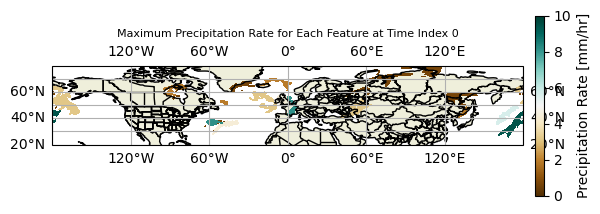

We can now not only see how the precipitation rates within each individual feature evolves, but also where new features pop up throughout the time indices selected! We have thus finished the detection algorithm, as we can thoroughly analyze precipitation features and how large-scale patterns of precipitation features evolve throughout the time period.

So far, we have focused on detecting features within the dataset. However, what if we wanted to track a specific feature throughout time? With the current methodology, we previously saw that a feature ID isn’t unique to each feature at each specific time step. Therefore, if we wanted to track a single feature, as we did previously, we would need to create an algorithm to compare each feature ID at each specific time period.

Precipitation Feature Tracking using Scipy¶

In order to track each feature, we need to get the centroid location of each feature. To do this, we consider all latitude and longitude points that are found within the precipitation feature that has an associated ID. We then convert those latitudes and longitudes into Cartesian coordinates, average them, and convert them back into latitudes and longitudes, thus giving the centroid location of the precipitation feature.

total_labeled_id_list = []
for i in range(len(data['time'])):
    precip_data = precip_feature(data, i)
    num_features = precip_data.max()
    labeled_id_list = []
    for j in range(1, num_features+1):
        feature_precip_data = np.argwhere(precip_data == j)
        latitudes = data['latitude'][feature_precip_data[:, 0]]
        longitudes = data['longitude'][feature_precip_data[:, 1]]
        longitudes = np.where(longitudes > 180, longitudes - 360, longitudes)
    
        ## Now we need to convert the latitudes/longitudes into cartesian coordinates.
        latitudes_rad = latitudes * np.pi/180
        longitudes_rad = longitudes * np.pi/180
        
        x = np.sum(np.cos(latitudes_rad) * np.cos(longitudes_rad))
        y = np.sum(np.cos(latitudes_rad) * np.sin(longitudes_rad))
        z = np.sum(np.sin(latitudes_rad))
        
        x /= len(latitudes_rad)
        y /= len(latitudes_rad)
        z /= len(latitudes_rad)
        
        central_lon = np.atan2(y,x) * 180/np.pi
        central_hypotenuse = np.sqrt(x*x + y*y)
        central_lat = np.atan2(z, central_hypotenuse) * 180/np.pi

        labeled_id_list.append((central_lon.data, central_lat.data, j))

    total_labeled_id_list.append(labeled_id_list)

We now have a list of all of the precipitation centroids within each time set. Now all we need to do is stitch the centroids together. In order to do this, we will say the center of the precipitation centroid can move no further than 200km in one hour. If it moves further than this, it will not be associated with a previous precipitation centroid at later hours. Although this choice is arbitrary, precipitation usually does not move in excess of 100km/hr, so if a centroid moves further than twice this distance, it likely represents structural re-organization and likely a different precipitation feature.

Before doing this though, let’s define a distance function.

def distance(lon1, lat1, lon2, lat2):
        radius = 6371
        dlat = math.radians(lat2 - lat1)
        dlon = math.radians(lon2 - lon1)
        a = math.sin(dlat/2) * math.sin(dlat/2) + math.cos(math.radians(lat1)) * math.cos(math.radians(lat2)) * math.sin(dlon/2) * math.sin(dlon/2)
        c = 2 * math.atan2(math.sqrt(a), math.sqrt(1-a))
        d = radius * c
        return d

first_time_step = total_labeled_id_list[0]
tracked_list = []
for point in first_time_step:
    time_index = 0

    lon = point[0]
    lat = point[1]
    ind = point[2]

    still_exists = True
    specific_track_list = [(lon, lat, ind)]
    while(still_exists):
        time_index += 1
        ## If the current time step is beyond the total number of time steps within the dataset, get out of here!
        if (time_index > len(data['time']) - 1):
            break

        ## Else, get time step data
        next_time_step = total_labeled_id_list[time_index]
        distances = np.zeros((len(next_time_step)))

        index = 0

        for feature in next_time_step:
            dist = distance(lon, lat, feature[0], feature[1])
            distances[index] = dist

            index += 1

        min_dist = np.argmin(distances)
        if (np.min(distances) < 200):
            new_lat = next_time_step[min_dist][1]
            new_lon = next_time_step[min_dist][0]
            new_ind = next_time_step[min_dist][2]
            specific_track_list.append((new_lon, new_lat, new_ind))
        else:
            still_exists = False
    tracked_list.append(specific_track_list)

Tracking the Number of Features Across Hours¶

We now have a complete list of all storms starting from the first time index going through to subsequent hours that a feature is tracked for. Let’s plot a distribution to see how long each storm is tracked for.

feature_length = np.empty(0)
for i in range(len(tracked_list)):
    feature_length = np.append(feature_length, len(tracked_list[i]) - 1) ## Every feature will have at least one point, since it is the starting lat/lon point. Need to subtract 1 to determine total number of hours.

feature_length = pd.Series(feature_length)
counts = feature_length.value_counts().sort_index()

counts.plot(kind='bar')
plt.xlabel('Number of Hours Each Tracked Feature Lasted')
plt.ylabel('Number of Features Tracked')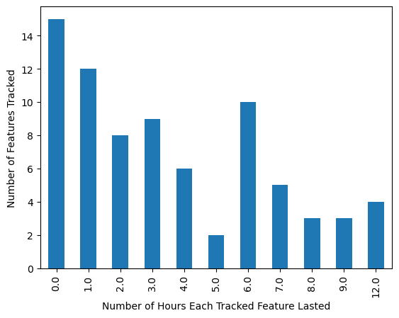

In general, we see a sharp drop-off in the number of features that lasted longer, with the majority of features from the first time index lasting only 0-1 hours. There are many fluctuations in later time steps, but overall, only a few features persist through the longest time steps.

Plotting the Tracking Algorithm Results¶

Now let’s show all of the tracked features from the first time index and how it evolves to the next time indices on a map.

def get_id_tracks(tracked_list, data, time_ind):
    id_at_time = np.empty(0)
    for i in range(len(tracked_list)):
        specific_track = tracked_list[i]
        if (len(specific_track) <= time_ind):
            continue
        time_index = specific_track[time_ind]
        id_at_time = np.append(id_at_time, time_index[2])
    
    precip_data = precip_feature(data, time_ind)
    mask = ~np.isin(precip_data, id_at_time)
    precip_data[mask] = 0
    return precip_data

Let’s plot!

## Let's create a function to write the figures necessary for the animation.

## Creating a colorbar across all frames.
vmin = 0
vmax = 10
levels = np.linspace(vmin, vmax, 10)
norm = mcolors.Normalize(vmin=vmin, vmax=vmax)
cmap='BrBG'

fig, ax = plt.subplots(subplot_kw={"projection": ccrs.PlateCarree()})

def func(i):
    ax.clear()
    lon2d, lat2d = np.meshgrid(no_minimal_precip['longitude'], no_minimal_precip['latitude'])
    subset_labeled_data = get_id_tracks(tracked_list, data, i).astype(float)
    subset_labeled_data[subset_labeled_data == 0] = np.nan
    plt.contourf(lon2d, lat2d, subset_labeled_data, cmap='tab20b', transform=ccrs.PlateCarree())
    ax.add_feature(cfeature.LAND)
    ax.add_feature(cfeature.BORDERS, edgecolor='black')
    ax.add_feature(cfeature.STATES, edgecolor='black')

    ax.set_extent([-180, 180, 20, 80])
    
    ax.add_feature(cfeature.COASTLINE, edgecolor='black')

    ax.set_title('Precip Features Tracked from Time Index 0 at Index ' + str(i))
    
    provinces = cfeature.NaturalEarthFeature(
        category='cultural',
        name='admin_1_states_provinces_lines',
        scale='50m',
        facecolor='none',
        edgecolor='black'
    )
    ax.add_feature(provinces)
    ax.gridlines(draw_labels=True)
    plt.tight_layout()
    return fig,


anim = FuncAnimation(fig, func, frames=len(data['time']), interval=300, blit=False)
HTML(anim.to_jshtml())
# anim.save('my_animation.gif', writer='pillow', fps=2)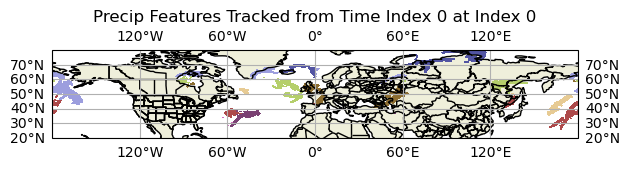

The results shown here are consistent with the bar graph. With increasing time index away from the idx=0, there are fewer and fewer features visible. This makes sense given the nature of some of these precipitation features, especially any convectively-related features. Some of the longer features likely represent some synoptic forcing that is persistent for a long period of time.

Last but not least, let’s plot the precipitation rate found within each contoured region. Although the raw precipitation rate field would be preferred, the maximum precipitation rate found within each feature is easier to visualize across the world and brings to light anomalous precipitation rate values found within each feature.

## Let's create a function to write the figures necessary for the animation.

## Creating a colorbar across all frames.
vmin = 0
vmax = 10
levels = np.linspace(vmin, vmax, 10)
norm = mcolors.Normalize(vmin=vmin, vmax=vmax)
cmap='BrBG'

fig, ax = plt.subplots(subplot_kw={"projection": ccrs.PlateCarree()})

sm = ScalarMappable(norm=norm, cmap=cmap)
sm.set_array([])
cbar = fig.colorbar(sm, ax=ax, pad=0.02, shrink=0.4)
cbar.set_label("Max. Precip. Rate [mm/hr]")

def func(i):
    ax.clear()
    lon2d, lat2d = np.meshgrid(no_minimal_precip['longitude'], no_minimal_precip['latitude'])
    subset_labeled_data = get_id_tracks(tracked_list, data, i).astype(float)
    subset_labeled_data[subset_labeled_data == 0] = np.nan
    maximum_precip = get_max_precip_data(data, i)
    maximum_precip[np.isnan(subset_labeled_data)] = np.nan
    plt.contourf(lon2d, lat2d, maximum_precip, cmap='BrBG', transform=ccrs.PlateCarree(), vmin=0, vmax=10)
    ax.add_feature(cfeature.LAND)
    ax.add_feature(cfeature.BORDERS, edgecolor='black')
    ax.add_feature(cfeature.STATES, edgecolor='black')

    ax.set_extent([-180, 180, 20, 80])
    
    ax.add_feature(cfeature.COASTLINE, edgecolor='black')

    ax.set_title('Precip Features Tracked from Time Index 0 at Index ' + str(i))
    
    provinces = cfeature.NaturalEarthFeature(
        category='cultural',
        name='admin_1_states_provinces_lines',
        scale='50m',
        facecolor='none',
        edgecolor='black'
    )
    ax.add_feature(provinces)
    ax.gridlines(draw_labels=True)
    plt.tight_layout()
    return fig,


anim = FuncAnimation(fig, func, frames=len(data['time']), interval=300, blit=False)
HTML(anim.to_jshtml())
# anim.save('my_animation.gif', writer='pillow', fps=2)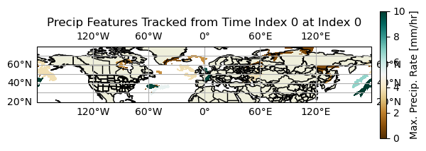

Although we can see wild fluctuations in the maximum precipitation rate for each feature, we can see that with increasing time, there are fewer features to track, consistent with the above figures/animations. The maximum precipitation rate features are also large enough to view across the entire domain.

Summary¶

Congratulations! 🎉 You now know how to develop and implement your very own detecting and tracking algorithm to detect precipitation features using Scipy. You should have a better understanding of how the Scipy label function works, how it handles merges and splits in precipitation features, and why a detection algorithm is simply insufficient to track precipitation features from one time to the next.

What’s next:¶

Add in additional examples using the maximum precipitation function.
Create examples showing raw precipitation rate instead of the maximum precipitation rate function.
Create a maximum precipitation rate function across the same tracked feature and plot the results.