Overview
Within this notebook, we will cover:
How to filter continuous SLP data do identify features of interest.
How to use matplotlib.pyplot’s
contour()function to identify coherent objects within the SLP fieldHow to track identified ETCs through successive time steps.
Prerequisites
| Concepts | Importance | Notes |
|---|---|---|
| xarray | Necessary | |
| matplotlib | Necessary | |
| Cartopy | Useful | |
| IPython | Useful | For inline animation |
Time to learn: 30 minutes
Import Packages
import numpy as np
import xarray as xr
import matplotlib.pyplot as plt
from matplotlib.animation import FuncAnimation
from IPython.display import HTML
from skimage.measure import label, regionprops
import matplotlib.colors as mcolors
from matplotlib.cm import ScalarMappable
import cartopy.crs as ccrs
from cartopy.util import add_cyclic_point
from matplotlib.path import Path
Let’s go through the basic steps to identify SLP features
Open the dataset using xarray
We have a small subset of hourly ERA5 Reanalysis dataset for Sea Level Pressure for 2022 November 1.
ds = xr.open_dataset("data/SLP_ex.nc")
da = ds["SLP"]
Define relevant set of parameters
Three values control what counts as a feature and how features are linked through time. We set them once here so the rest of the notebook stays readable.
threshold- Grid cells below this value are flagged as part of a low. Everything at or above it is background. ERA5 reports sea-level pressure in pascals, so this is about 1000 hPa.min_area- The smallest feature we keep, measured in grid cells. Below threshold blobs smaller than 20 cells are treated as noise and dropped. Since we haven’t smoothed the field yet, this is what stops single-cell specks from being counted as a feature.min_overlap- The matching rule for tracking. A feature at one timestep is identified with a feature at the next when they share at least 20% overlap. Below that level, they’re treated as separate features. Lower values follow faster moving systems but risk false links and higher values require a feature to barely move between steps.
threshold = 100000
min_area = 20
min_overlap = 0.2
Get the latitude and longitude 2d meshgrid for plotting
To plot SLP with contour(), we first create 2D latitude–longitude grids. The SLP dataset is at a resolution of 1° × 1°.
lat = da[da.dims[1]].values
lon = da[da.dims[2]].values

# if lat/lon are 1D, make 2D grids for contourf/contour
lon2d, lat2d = np.meshgrid(lon, lat)
Select low SLP features less than a threshold using matplotlib contour()
This function detects low-pressure SLP features from a single time step using Matplotlib contours. First, it draws the contour line at the chosen SLP threshold, such as 1000 or 1005 hPa. Each closed contour segment is then converted into a filled polygon mask, which marks the grid cells inside that contour. Since we only want low-pressure systems, the mask is further restricted to grid points where SLP <= threshold. Very small objects are removed using the min_area limit. For each remaining feature, the function stores a frame-specific feature_id, the feature mask, and its centroid location as row and column indices.
def detect_features_matplotlib(field, threshold=100000, min_area=20):
    ny, nx = field.shape

    yy, xx = np.mgrid[0:ny, 0:nx]
    points = np.column_stack([xx.ravel(), yy.ravel()])

    # Draw contour at the SLP threshold
    fig, ax = plt.subplots()
    cs = ax.contour(field, levels=[threshold])
    plt.close(fig)

    features = []
    feature_id = 1

    for seg in cs.allsegs[0]:

        if len(seg) < 3:
            continue

        path = Path(seg)

        # Convert contour polygon into a filled mask
        mask = path.contains_points(points).reshape(ny, nx)

        # Keep only the low-pressure side of the contour
        mask = mask & (field <= threshold)

        # Remove tiny features
        if mask.sum() < min_area:
            continue

        # Centroid from mask grid cells
        y, x = np.where(mask)
        centroid = (y.mean(), x.mean())   # row, col

        features.append({
            "feature_id": feature_id,
            "mask": mask,
            "centroid_rc": centroid,
        })

        feature_id += 1

    return features
Test it out for the first time step
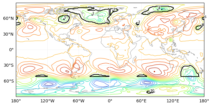
Let’s take a look at the labelled feature at time = 0 which at 2022 November 1 00:00 UTC.
t = 0
slp = da.isel(time=t).values
We call the detect_features_matplotlib() function with the parameters set above
labels = detect_features_matplotlib(slp, threshold=threshold, min_area=min_area)levels = np.linspace(float(da.min()), float(da.max()), 16)
fig, ax = plt.subplots(
figsize=(8, 4),
subplot_kw={"projection": ccrs.PlateCarree()}
)
# colored SLP contour lines
ax.contour(
lon2d, lat2d, slp,
levels=levels,
cmap="turbo",
linewidths=0.9,
transform=ccrs.PlateCarree()
)
for feat in labels:
mask = feat["mask"]
ax.contour(
lon2d,
lat2d,
mask.astype(int),
levels=[0.5],
colors="black",
linewidths=1.6,
transform=ccrs.PlateCarree()
)
y, x = feat["centroid_rc"] # row, column
iy = int(round(y))
ix = int(round(x))
ax.plot(
lon[ix],
lat[iy],
"ko",
ms=3,
transform=ccrs.PlateCarree()
)
ax.text(
lon[ix],
lat[iy],
str(feat["feature_id"]),
fontsize=8,
color="black",
ha="left",
va="bottom",
transform=ccrs.PlateCarree(),
bbox=dict(facecolor="white", edgecolor="none", alpha=0.7, pad=1)
)
ax.coastlines(color="0.55", linewidth=0.6)
gl = ax.gridlines(
draw_labels=True,
linewidth=0.4,
color="0.5",
alpha=0.25,
linestyle="--"
)
gl.top_labels = False
gl.right_labels = False
#ax.set_title(f"Matplotlib contour-tracked SLP features | time index = {t}")
plt.show()
Let’s track SLP Features Over Time
This function tracks the Matplotlib-detected SLP features through time. It starts with an empty list to store the tracked features, an empty dictionary to store features from the previous time step, and a counter for assigning new track_id values. For each time step, the function first detects the low-pressure features using detect_features_matplotlib(). It then compares each current feature mask with the masks from the previous time step. The overlap is calculated as the fraction of the current feature that overlaps with an older feature. If the overlap is larger than the chosen min_overlap threshold, the current feature keeps the same track_id. If there is not enough overlap, the feature is treated as a new object and receives a new track_id. For each frame, the function stores the persistent track_id, the frame-specific feature_id, the centroid location, the mask, and the overlap value. The final output is a time-ordered list of tracked SLP features that can be used for plotting or animation.
def track_slp_features_matplotlib(
    da,
    threshold=100000,
    min_area=20,
    min_overlap=0.2,
):
    """
    Track SLP low-pressure features detected using Matplotlib contours.

    Tracking rule:
        A feature keeps the same track_id if it overlaps enough
        with a feature from the previous time step.
    """

    tracked = []
    prev = {}
    next_track_id = 1

    for t in range(da.sizes["time"]):

        field = da.isel(time=t).values

        # Detect features at this time step
        features = detect_features_matplotlib(
            field,
            threshold=threshold,
            min_area=min_area
        )

        current = {}
        frame_info = []

        for feat in features:

            mask = feat["mask"]

            best_id = None
            best_overlap = 0.0

            for track_id, old_mask in prev.items():

                overlap = np.logical_and(mask, old_mask).sum() / mask.sum()

                if overlap > best_overlap:
                    best_overlap = overlap
                    best_id = track_id

            # Assign new ID if no strong overlap with previous features
            if best_overlap < min_overlap:
                best_id = next_track_id
                next_track_id += 1

            current[best_id] = mask

            frame_info.append({
                "track_id": best_id,
                "feature_id": feat["feature_id"],     # frame-specific ID
                "centroid_rc": feat["centroid_rc"],   # row, col
                "mask": mask,
                "overlap": best_overlap,
            })

        tracked.append(frame_info)
        prev = current

    return tracked
tracked_mpl = track_slp_features_matplotlib(
da,
threshold=threshold,
min_area=20,
min_overlap=0.2,
)Let’s look at the animation of the SLP features
lat = da[da.dims[1]].values
lon = da[da.dims[2]].values
lon2d, lat2d = np.meshgrid(lon, lat)

levels = np.linspace(float(da.min()), float(da.max()), 16)

fig, ax = plt.subplots(
    figsize=(8, 4),
    subplot_kw={"projection": ccrs.PlateCarree()}
)

def update(t):
    ax.clear()

    field = da.isel(time=t).values

    # colored SLP contour lines
    ax.contour(
        lon2d, lat2d, field,
        levels=levels,
        cmap="turbo",
        linewidths=0.9,
        transform=ccrs.PlateCarree()
    )

    # tracked feature outlines and IDs
    for feat in tracked_mpl[t]:
        mask = feat["mask"]

        ax.contour(
            lon2d, lat2d, mask.astype(int),
            levels=[0.5],
            colors="black",
            linewidths=1.6,
            transform=ccrs.PlateCarree()
        )

        y, x = feat["centroid_rc"]
        iy = int(round(y))
        ix = int(round(x))

        ax.plot(
            lon[ix], lat[iy],
            "ko", ms=3,
            transform=ccrs.PlateCarree()
        )

        ax.text(
            lon[ix], lat[iy],
            str(feat["track_id"]),
            fontsize=8,
            color="black",
            ha="left",
            va="bottom",
            transform=ccrs.PlateCarree(),
            bbox=dict(facecolor="white", edgecolor="none", alpha=0.7, pad=1)
        )

    ax.coastlines(color="0.55", linewidth=0.6)

    gl = ax.gridlines(
        draw_labels=True,
        linewidth=0.4,
        color="0.5",
        alpha=0.25,
        linestyle="--"
    )
    gl.top_labels = False
    gl.right_labels = False

    #ax.set_title(f"Matplotlib contour-tracked SLP features | time index = {t}")

anim = FuncAnimation(
    fig,
    update,
    frames=da.sizes["time"],
    interval=300,
    blit=False,
)

plt.close(fig)
HTML(anim.to_jshtml())This animation shows the evolution of SLP through time using the overlap tracking method. The numeric annotations help follow the features. There seems to be a gap in tracking extratropical southern hemisphere which needs further inspection.
Summary
In this recipe, we identify low sea level pressure (SLP) features globally and track them through time. We use matplotlib.pyplot.contour() to detect coherent low-pressure objects. We track tracking identified features between time steps using spatial overlap percentage and made visualization for one time step and a hourly animation for duration of 1 day.
What’s next?
Adding smoothing or noise filtering before feature detection.
Comparing this contour-based method with scikit-image and scipy object-labeling approaches.
Extracting region properties such as area, centroid, perimeter, and intensity.
Testing sensitivity to different SLP thresholds.
Adding explicit split and merge detection during tracking.