Great Circle Terminology
Overview
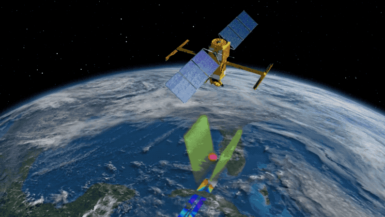
Great circles are powerful tools and historically were commonly used in the navigation of ships. Today, they are a common tool for pilots to plot paths “as-the-crow-flies” as well as in geoscience when working with remote sensing via satellites that pass over the globe in long curved arcs.
The mathematics of great circles make use of spherical geometry, where, rather than lines, long arcs are drawn along the surface of a sphere. While spherical geometry played an important role historically in the fields of astronomy and navigation, its teaching has largely fallen out of favor since the 1950’s making finding comphrenshive resources difficult.
This notebook will cover the important and unique terminology used when working with great circles and spherical geometry.
Great Circles
Spherical Geometry
Ellipsoids vs. Spheres
Geodesy
Python Packages
A Note on Resources
Prerequisites
Time to learn: 20 minutes
Great Circles
Great Circle Path vs. Great Circle Arc
A great circle path is the full path formed by the intersection of a plane which also passes through the center of the sphere. For example, the equator is an example of a great circle path on the Earth. The equator can be imagined as the path formed by a plane cutting through the center of the planet and intersecting the center. A great circle path is a closed path (-180 to 180 degrees longitude) that forms around the sphere.
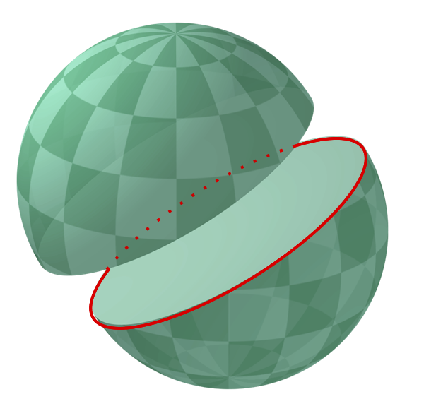
All great circles:
Intersect the center of the Earth
Divide the Earth in half
A great circle arc is a small subsection of a great circle path, representing an arc between two points on the surface of a sphere. The arc will represent the shortest distance between any two points on the surface of the Earth. An arc can be formed with:
Two points
Or: One point, a bearing, and a distance
Spherical Geometry
Spherical Trigonometry
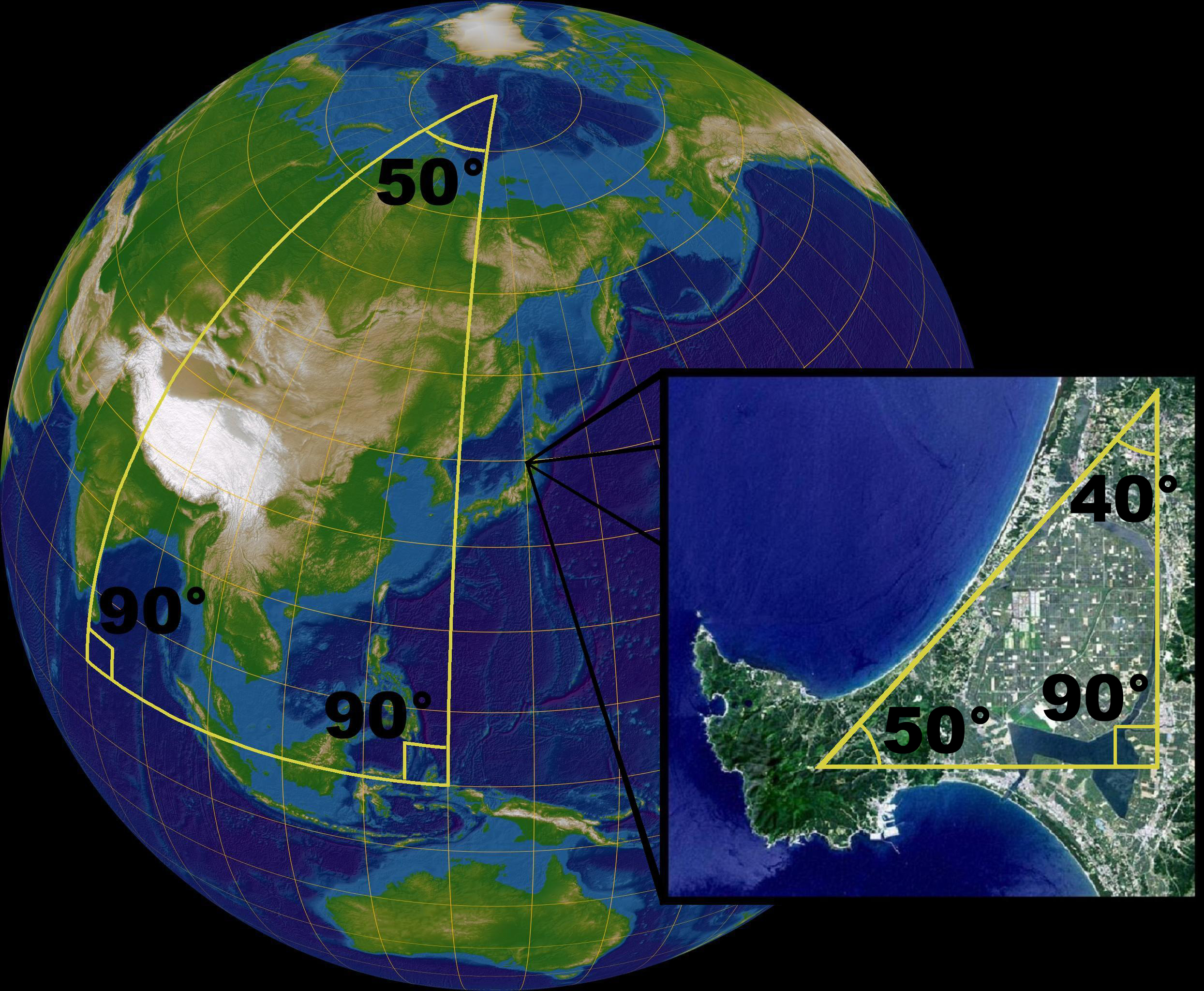
Spherical geometry (and one of it important branches: spherical trigonometry) provide calculations based on the relationshsips between the sides and angles on a sphere that are commonly used in right-angled triangles. Spheres are unique since unlike flat surfaces, spherical triangles can have internal angles that add up to more than 180 degrees.
For example, imagine you fly a plane from the Philippines directly North until you reach the top of the Earth (at the North Pole). Then, you turn the plane 50 degrees, and fly down again until you arrive at the starting latitude of Philippines, off the coast of India. Once you have returned to your same starting latitude, you turn 90 degrees and return to the Philippines. By this point, you will have made two 90 degree turns (off the coast of India and the Philippines). So, all the internal angles combined to make this triangle along the Earth are 230 degrees (90 + 90 + 50).
The sum of the angles of a spherical triangle is not equal to 180°. A sphere is a curved surface, but locally the laws of the flat (planar) Euclidean geometry are good approximations. In a small triangle on the face of the earth, the sum of the angles is only slightly more than 180 degrees
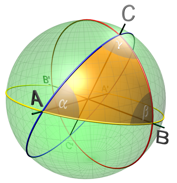
Like a flat 2D triangle, spherical triangles have the own sine and cosine identities that can be used to solve internal angles and the length of sides.
Law of Cosines
“The cosine rule is the fundamental identity of spherical trigonometry: all other identities, including the sine rule, may be derived from the cosine rule” (Wikipedia)
The spherical law of cosines states that for the angles A, B, C and opposite sides a, b, c:
Law of Sines
The law of sines can be constructed from the law of cosines, where the spherical law of sines states that for the angles A, B, and C and the opposite of the sides a, b, c:
Ellipsoids vs. Spheres
The earth is not round, instead it is an irregular ellipsoid known as a an oblate spheroid where the poles are slightly flatter and the equator bulges out. Spherical trigonometry typically assumes that calculations are occurring on a perfect sphere. For much of history this approximiation was accurate enough to allow ships to find their way to ports, but with increasingly technologically advanced and precise tools (like satellites) this discrepancy becomes more and more pronounced. Any calculation on Earth that assumes the planet is a perfect sphere, and without additional corrections, will contain an error up to 0.3% (22 km) (see more).
The various Python geodetic tools that we will in this cookbook will attempt to account for these errors by making use of different sized ellipsoids with flattening parameters.
Geodesy
Geodesy is the complex science of measuring the Earth’s size and shape (as well as orientation and gravity field, but that is out of the scope of this notebook).
The methods of measuring Earth have changed dramatically through history from physical survey tools to modern GPS.
Geodesic
A geodesic is the shortest curved path between any two points on a surface. A “straight line” on the surface of a curved surface (like a sphere) will form an arc. A great circle arc is a special type of arc that is formed by a plane intersecting the center of a sphere.
If an insect is placed on a surface and continually walks “forward”, by definition it will trace out a geodesic
This is especially apparent when working with satellite data where the apparent “straight path” that a satellite will trace across the the surface of a planet turns into an arc or curve on a map.
Python Packages
For the purpose of this notebook we will be taking advantage of two geoscience Python packages:
pyproj and geopy both take advantage of different types of (optional) ellipsoids, where a is the radius (semi-major or equatorial axis radius) in meters, rf is the reciprocal flattening, and b (where available) is the semi-minor axis (polar axis radius).
import pyproj
for key in pyproj.list.get_ellps_map().keys():
    print(f"{key} = {pyproj.list.get_ellps_map()[key]}")
MERIT = {'a': 6378137.0, 'rf': 298.257, 'description': 'MERIT 1983'}
SGS85 = {'a': 6378136.0, 'rf': 298.257, 'description': 'Soviet Geodetic System 85'}
GRS80 = {'a': 6378137.0, 'rf': 298.257222101, 'description': 'GRS 1980(IUGG, 1980)'}
IAU76 = {'a': 6378140.0, 'rf': 298.257, 'description': 'IAU 1976'}
airy = {'a': 6377563.396, 'rf': 299.3249646, 'description': 'Airy 1830'}
APL4.9 = {'a': 6378137.0, 'rf': 298.25, 'description': 'Appl. Physics. 1965'}
NWL9D = {'a': 6378145.0, 'rf': 298.25, 'description': 'Naval Weapons Lab., 1965'}
mod_airy = {'a': 6377340.189, 'b': 6356034.446, 'description': 'Modified Airy'}
andrae = {'a': 6377104.43, 'rf': 300.0, 'description': 'Andrae 1876 (Den., Iclnd.)'}
danish = {'a': 6377019.2563, 'rf': 300.0, 'description': 'Andrae 1876 (Denmark, Iceland)'}
aust_SA = {'a': 6378160.0, 'rf': 298.25, 'description': 'Australian Natl & S. Amer. 1969'}
GRS67 = {'a': 6378160.0, 'rf': 298.247167427, 'description': 'GRS 67(IUGG 1967)'}
GSK2011 = {'a': 6378136.5, 'rf': 298.2564151, 'description': 'GSK-2011'}
bessel = {'a': 6377397.155, 'rf': 299.1528128, 'description': 'Bessel 1841'}
bess_nam = {'a': 6377483.865, 'rf': 299.1528128, 'description': 'Bessel 1841 (Namibia)'}
clrk66 = {'a': 6378206.4, 'b': 6356583.8, 'description': 'Clarke 1866'}
clrk80 = {'a': 6378249.145, 'rf': 293.4663, 'description': 'Clarke 1880 mod.'}
clrk80ign = {'a': 6378249.2, 'rf': 293.4660212936269, 'description': 'Clarke 1880 (IGN).'}
CPM = {'a': 6375738.7, 'rf': 334.29, 'description': 'Comm. des Poids et Mesures 1799'}
delmbr = {'a': 6376428.0, 'rf': 311.5, 'description': 'Delambre 1810 (Belgium)'}
engelis = {'a': 6378136.05, 'rf': 298.2566, 'description': 'Engelis 1985'}
evrst30 = {'a': 6377276.345, 'rf': 300.8017, 'description': 'Everest 1830'}
evrst48 = {'a': 6377304.063, 'rf': 300.8017, 'description': 'Everest 1948'}
evrst56 = {'a': 6377301.243, 'rf': 300.8017, 'description': 'Everest 1956'}
evrst69 = {'a': 6377295.664, 'rf': 300.8017, 'description': 'Everest 1969'}
evrstSS = {'a': 6377298.556, 'rf': 300.8017, 'description': 'Everest (Sabah & Sarawak)'}
fschr60 = {'a': 6378166.0, 'rf': 298.3, 'description': 'Fischer (Mercury Datum) 1960'}
fschr60m = {'a': 6378155.0, 'rf': 298.3, 'description': 'Modified Fischer 1960'}
fschr68 = {'a': 6378150.0, 'rf': 298.3, 'description': 'Fischer 1968'}
helmert = {'a': 6378200.0, 'rf': 298.3, 'description': 'Helmert 1906'}
hough = {'a': 6378270.0, 'rf': 297.0, 'description': 'Hough'}
intl = {'a': 6378388.0, 'rf': 297.0, 'description': 'International 1924 (Hayford 1909, 1910)'}
krass = {'a': 6378245.0, 'rf': 298.3, 'description': 'Krassovsky, 1942'}
kaula = {'a': 6378163.0, 'rf': 298.24, 'description': 'Kaula 1961'}
lerch = {'a': 6378139.0, 'rf': 298.257, 'description': 'Lerch 1979'}
mprts = {'a': 6397300.0, 'rf': 191.0, 'description': 'Maupertius 1738'}
new_intl = {'a': 6378157.5, 'b': 6356772.2, 'description': 'New International 1967'}
plessis = {'a': 6376523.0, 'b': 6355863.0, 'description': 'Plessis 1817 (France)'}
PZ90 = {'a': 6378136.0, 'rf': 298.25784, 'description': 'PZ-90'}
SEasia = {'a': 6378155.0, 'b': 6356773.3205, 'description': 'Southeast Asia'}
walbeck = {'a': 6376896.0, 'b': 6355834.8467, 'description': 'Walbeck'}
WGS60 = {'a': 6378165.0, 'rf': 298.3, 'description': 'WGS 60'}
WGS66 = {'a': 6378145.0, 'rf': 298.25, 'description': 'WGS 66'}
WGS72 = {'a': 6378135.0, 'rf': 298.26, 'description': 'WGS 72'}
WGS84 = {'a': 6378137.0, 'rf': 298.257223563, 'description': 'WGS 84'}
sphere = {'a': 6370997.0, 'b': 6370997.0, 'description': 'Normal Sphere (r=6370997)'}
By default, pyproj has more options for ellipsoids, but several of these ellipsoids are also available in geopy as well, with a radius in kilometers instead of meters
from geopy import distance
for key in distance.ELLIPSOIDS.keys():
    print(f"{key} = {distance.ELLIPSOIDS[key]}")
WGS-84 = (6378.137, 6356.7523142, 0.0033528106647474805)
GRS-80 = (6378.137, 6356.7523141, 0.003352810681182319)
Airy (1830) = (6377.563396, 6356.256909, 0.0033408506414970775)
Intl 1924 = (6378.388, 6356.911946, 0.003367003367003367)
Clarke (1880) = (6378.249145, 6356.51486955, 0.003407561378699334)
GRS-67 = (6378.16, 6356.774719, 0.003352891869237217)
The standard reference ellipsoid for working with Earth is WGS-84
geopy by default makes use of WGS-84 which is a a unified global ellipsoid model that is used for GPS collected from satellites to calculate extremely preise measurements of the Earth. For the purpose of this notebook, this is the ellipsoid model we will be working with.
print(pyproj.list.get_ellps_map()["WGS84"])
print(distance.ELLIPSOIDS["WGS-84"])
{'a': 6378137.0, 'rf': 298.257223563, 'description': 'WGS 84'}
(6378.137, 6356.7523142, 0.0033528106647474805)
WGS-84 is an ellipsoid with a semi-major axis of 6378137.0 meters, an inverse (reciprocal) flattening feature of 298.257223563, and a flattening factor of 0.0033528106647474805.
An Important Note on Resources
Spherical geometry and resources associated with working with great circles can be difficult to find
Here are a list of some for working mathematically with great circles:
“Heavenly Mathematics: The Forgotten Art of Spherical Trigonometry” by Glen Van Brummelen
“Spherical Trigonometry: A Comprehensive Approach” by Ira Arevalo Fajardo
Summary
A great circle is formed by a plane intersecting a sphere and the center, like the equator.
Great circles make use of spherical geometry to measure features on the curved surface of a unit sphere. However, planets like Earth are not perfect spheres and to account for the error are combined with geodesic calculations to reduce the error in final calculations.
What’s next?
How do we measure a specific place on the Earth or any sphere?
Up next: Coordinates and Great Circles