From Earth, a geostationary satellite looks like it is always in the same place, because it moves in the same direction and at the same rate the Earth spins. Image credit: NASA Solar System Exploration

Coordinate Types¶

Overview¶

Great circles can use a diverse variety of different types of coordinates. This notebook will cover the different types of coordinates that are used when calculating great circles and how to convert between them. This notebook will also begin to show how to plot coordinates and their associated great circle arcs on a map of Earth.

Types of Coordinates
Convert Coordinates to All Coordinate Types
Plot Coordinates on a World Map

Prerequisites¶

Concepts	Importance	Notes
Numpy	Necessary	Used to work with large arrays
Pandas	Necessary	Used to read in and organize data (in particular dataframes)
Intro to Cartopy	Helpful	Will be used for adding maps to plotting
Matplotlib	Helpful	Will be used for plotting

Time to learn: 20 minutes

Imports¶

import numpy as np                                     # working with degrees and radians
import pandas as pd                                    # working with data and dataframes

import matplotlib.pyplot as plt                        # plotting a graph
from cartopy import crs as ccrs, feature as cfeature   # plotting a world map

Types of Coordinates¶

Geodetic Coordinates¶

Geodetic coordinates are latitude and longtiude and are measured from -90° South to 90° North and -180° East to 180° West measured from Greenwich. Geodetic coordinates also include a geodetic height, which on Earth represents the radius of the planet.

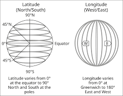
Longitude lines are perpendicular to and latitude lines are parallel to the Equator from Wikipedia

0 degrees latitude represents the middle of Earth at the equator while 0 degrees longitude was arbitrarily chosen to lie in the Royal Observatory in Greenwich (in London, England). This is known as the Prime Meridian and due to its arbitrary definition the location of the Prime Meridian have varied throughout history.

Cartesian Coordinates¶

Cartesian coordinates describe points in space based on perpendicular axis lines that meet at a single point of origin, where any point’s position is described based on the distance to the origin along xyz axis.

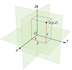
A three dimensional Cartesian coordinate system, with origin O and axis lines X, Y and Z, oriented as shown by the arrows. The tick marks on the axes are one length unit apart. The black dot shows the point with coordinates x = 2, y = 3, and z = 4, or (2, 3, 4) from Wikipedia

Image Source: Three Dimensional Cartesian Coordinate System

How to Convert from Geodetic to Cartesian Coordinates¶

Assuming the Earth’s radius is 6378137 meters then:

x = radius * cos(latitude) * cos(longitude)

(1)

y = radius * cos(latitude) * sin(longitude)

(2)

z = radius * sin(latitude)

(3)

However, on a unit sphere, we can consider the radius to be 1.

def cartesian_coordinates(latitude=None, longitude=None):
    radius = 1
    latitude = np.deg2rad(latitude)
    longitude = np.deg2rad(longitude)
    cart_x = radius * np.cos(latitude) * np.cos(longitude)
    cart_y = radius * np.cos(latitude) * np.sin(longitude)
    cart_z = radius * np.sin(latitude)
    return cart_x, cart_y, cart_z

Spherical Coordinates¶

Spherical coordinates describe points in space based on three values: radial distance (rho, r) along the radial line between point and the origin, polar angle (theta, θ) between the radial line and the polar axis, and azimuth angle (phi, φ) which is the angle of rotation of the radial line around the polar axis. With a fixed radius, the 3-point coordinates (r, θ, φ) provide a coordinate along a sphere.

Radial distance (r): distance from center to surface of sphere
Polar angle (θ): angle between radial line and polar axis
Azimuth angle (φ): angle around polar axis

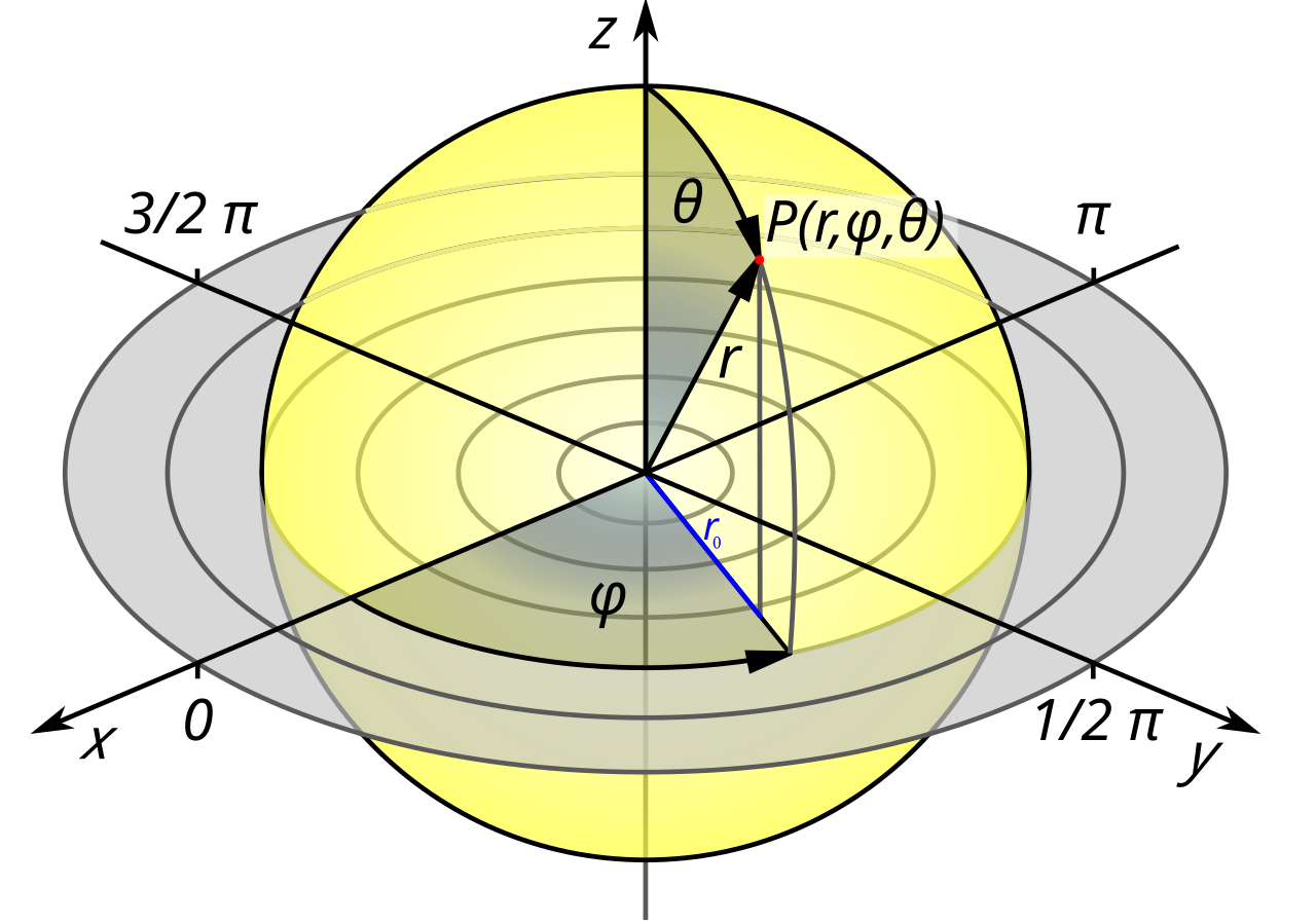
Spherical Coordinate Description from Wikipedia

Image Source: Wikipedia - Spherical Coordinate System

Convert from Cartesian to Spherical Coordinates¶

ρ^2 = x^2 + y^2 + z^2

(4)

tan(θ) = \frac{y}{x}

(5)

φ = arccos(\frac{x}{\sqrt{x^2 + y^2 + z^2}})

(6)

Where, rho (ρ), theta (θ), phi (φ):

ρ = \sqrt{x^2 + y^2 + z^2}

(7)

θ = arctan(\frac{y}{x})

(8)

φ = arccos(\frac{x}{ρ})

(9)

def cartesian_to_spherical_coordinates(cart_x=None, cart_y=None, cart_z=None):
    rho = np.sqrt(cart_x**2 + cart_y**2 + cart_z**2)
    theta = np.arctan(cart_y/cart_x)
    phi = np.arccos(cart_z / rho)
    return rho, theta, phi

Polar Coordinates¶

Polar coordinates are a combination of latitude, longitude, and altitude from the center of the sphere (based on the radius).

Convert Geodetic to Polar Coordinates¶

Assuming the Earth’s radius is 6378137 meters then:

x = cos(latitude) * cos(longitude) * radius

(10)

y = cos(latitude) * sin(longitude) * radius

(11)

z = sin(latitude) * radius

(12)

def polar_coordinates(latitude=None, longitude=None):
    earth_radius = 6378137  # meters
    latitude = np.deg2rad(latitude)
    longitude = np.deg2rad(longitude)
    polar_x = np.cos(latitude) * np.sin(longitude) * earth_radius
    polar_y = np.cos(latitude) * np.cos(longitude) * earth_radius
    polar_z = np.sin(latitude) * earth_radius
    return polar_x, polar_y, polar_z

Convert City Coordinates to All Coordinate Types¶

This notebook contains a list of locations (location_coords.txt) (see here) with their associated latitude and longitude coordinates. We will use the functions defined above to convert latitude/longitude to all coordinate types and save the output to a new file (location_full_coords.txt). In the future, different functions will require different coordinates to complete their calculations, so it is useful to have all these coordinates values known in advance.

Display Coordinates of Cities¶

First, we will read in the latitude and longitude coordinates from saved text file location.txt and save the details in a pandas dataframe:

location_df = pd.read_csv("../location_coords.txt")
location_df = location_df.rename(columns=lambda x: x.strip()) # strip excess white space from column names and values
location_df

Add Columns for Additional Coordinate Types¶

We will now add columns to the dataframe for each of the three additional coordinate types: cartesian, spherical, and polar. And finally, we will save the output to a new file we can reference in the future location_full_coords.txt.

location_df["cart_x"], location_df["cart_y"], location_df["cart_z"] = cartesian_coordinates(location_df["latitude"],
                                                                                            location_df["longitude"])
location_df["rho"], location_df["theta"], location_df["phi"] = cartesian_to_spherical_coordinates(location_df["cart_x"],
                                                                                                  location_df["cart_y"],
                                                                                                  location_df["cart_z"])
location_df["polar_x"], location_df["polar_y"], location_df["polar_z"] = polar_coordinates(location_df["latitude"],
                                                                                           location_df["longitude"])

location_df

# Save Output to a New Text File
location_df.to_csv("../location_full_coords.txt", index=False)

Plot Coordinates¶

Coordinates can be hard to visualize internally, so let’s plot them on a world map of Earth. A common plotting tool in Python is matplotlib, but to include a world map we will also use cartopy which stores many different kinds of maps of Earth.

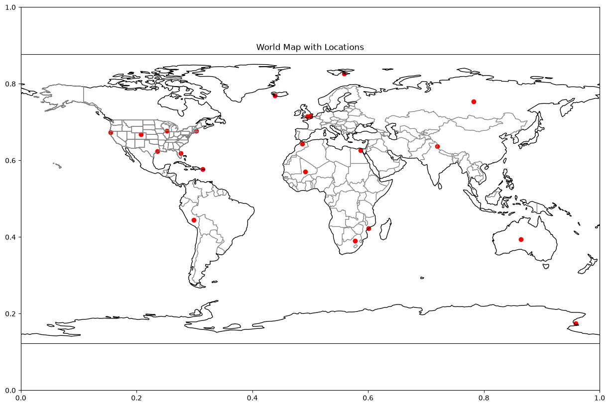
World Map¶

To generate a full world map, we need the full range of longitude and latitude from -180 degrees to 180 degrees and -90 degrees to 90 degrees.

longitude east = 180

longitude west = -180

latitude north = 90

latitude south = -90

# Setup Matplotlib Plot Figure with a size of 15 by 10
fig = plt.subplots(figsize=(15, 10)) 

# Overlay a plot of the Plate Carree Projection of Earth (a flat map of the planet)
projection_map = ccrs.PlateCarree()
ax = plt.axes(projection=projection_map)

# Plot the full range of latitude/longitude
lon_west, lon_east, lat_south, lat_north = -180, 180, -90, 90
ax.set_extent([lon_west, lon_east, lat_south, lat_north], crs=projection_map)

# Include the coastlines (in black) as well as the border of the continents and the states in the US (in grey)
ax.coastlines(color="black")
ax.add_feature(cfeature.BORDERS, edgecolor='grey')
ax.add_feature(cfeature.STATES, edgecolor="grey")
    
# Plot each location on the map as a red dot
longitudes = location_df["longitude"] # longitude
latitudes = location_df["latitude"]   # latitude
plt.scatter(longitudes, latitudes, c="red")

# Set the title of the map and display
plt.title("World Map with Locations")
plt.show()

/home/runner/micromamba/envs/cookbook-gc/lib/python3.13/site-packages/cartopy/io/__init__.py:242: DownloadWarning: Downloading: https://naturalearth.s3.amazonaws.com/110m_physical/ne_110m_coastline.zip
  warnings.warn(f'Downloading: {url}', DownloadWarning)

/home/runner/micromamba/envs/cookbook-gc/lib/python3.13/site-packages/cartopy/io/__init__.py:242: DownloadWarning: Downloading: https://naturalearth.s3.amazonaws.com/110m_cultural/ne_110m_admin_0_boundary_lines_land.zip
  warnings.warn(f'Downloading: {url}', DownloadWarning)

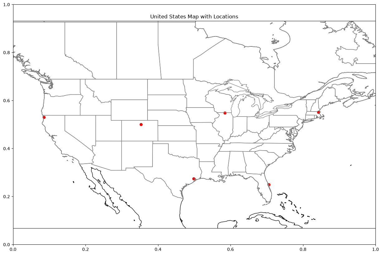
United States Map¶

Sometimes you don’t need to view the whole map, but a sub-section. For example, if we only wanted to view the US on a world map we would need a small range of latitude/longtiude coordinates

longitude east = -60

longitude west = -130

latitude north = 60

latitude south = 20

# Setup Matplotlib Plot Figure with a size of 15 by 10
fig = plt.subplots(figsize=(15, 10)) 

# Overlay a plot of the Plate Carree Projection of Earth (a flat map of the planet)
projection_map = ccrs.PlateCarree()
ax = plt.axes(projection=projection_map)

# Plot the a range of latitude/longitude to encompass the US
lon_west, lon_east, lat_south, lat_north = -130, -60, 20, 60
ax.set_extent([lon_west, lon_east, lat_south, lat_north], crs=projection_map)

# Include the coastlines (in black) as well as the border of the continents and the states in the US (in grey)
ax.coastlines(color="black")
ax.add_feature(cfeature.BORDERS, edgecolor='grey')
ax.add_feature(cfeature.STATES, edgecolor="grey")
    
# Plot each location on the map as a red dot
longitudes = location_df["longitude"] # longitude
latitudes = location_df["latitude"]   # latitude
plt.scatter(longitudes, latitudes, c="red")

# Set the title of the map and display
plt.title("United States Map with Locations")
plt.show()

/home/runner/micromamba/envs/cookbook-gc/lib/python3.13/site-packages/cartopy/io/__init__.py:242: DownloadWarning: Downloading: https://naturalearth.s3.amazonaws.com/50m_cultural/ne_50m_admin_1_states_provinces_lakes.zip
  warnings.warn(f'Downloading: {url}', DownloadWarning)

Summary¶

Coordinates on the Earth are measured in many different systems: Geodetic (latitude/longitude), Cartesian, Spherical, and Polar. In the next notebooks, these coordinates will be used to create great circle arcs and paths based on vector vector calculations.

In Python, coordinates can be mapped on to a world map via matplotlib and cartopy.

What’s next?¶

Now that we have coordinates, it’s time to connect them to create great circles!

Up Next: Great Circle arcs and paths

Resources and references¶

Foundations

Great Circle Terminology

Tutorials

Great Circle Arcs and Path