xESMF Demo using SEVIER dataset for Machine Learning Preperation

Thomas Martin ThomasMGeo

Sept 2 - 2022

Overview¶

This is a quick (~20 minute) notebook that will cover how to use xESMF to regrid with xarray on a dataset. This notebooks will heavily borrow from this repo: https://github.com/ai2es/WAF_ML_Tutorial_Part1 & this paper https://proceedings.neurips.cc/paper/2020/file/fa78a16157fed00d7a80515818432169-Paper.pdf . Randy Chase (dopplershift on github) is thanked for dataset prep and previous work!

Prerequisits¶

Working knowldge of xarray, matplotlib, and numpy is beneficial. This is not designed to be an introduction to any of those packages.

Imports¶

import numpy as np
import xarray as xr
import xesmf as xe

# Plotting utilities
import seaborn as sns
import matplotlib.pyplot as plt

Watermark is great repo to track versions when sharing work with notebooks. xESMF can be a little tricky to install, highly reccomend to install via conda instread of pip.

%load_ext watermark
%watermark --iversions

numpy     : 2.3.4
xarray    : 2025.10.1
seaborn   : 0.13.2
matplotlib: 3.10.7
xesmf     : 0.8.10

Dataset Load¶

file = '../data/onestorm.nc' # netcdf file

#open an example storm 
ds = xr.open_dataset(file)
#see the data by printing ds. By putting at the bottom of the cell, it is automatically printed
ds

We will be using this single dataset for the entirety of the notebook

plt.figure(figsize=(9,6))
#show all x pixels (:) and all y pixels (:) and the first time step, with a Grey colorscale, and the color min 0 and color max 1. 
plt.imshow(ds.visible.isel(t=0)[:,:]*1e-4,cmap='Greys_r',vmin=0,vmax=1) # At timestep 0

#show us the colorbar 
plt.colorbar(label='Visible Reflectance Factor')
#a function that cleans some of the figure up. 
plt.tight_layout()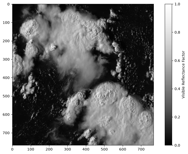

Let’s Zoom in one one patch, to gain some intuition on how satellite data is used in Machine Learning (ML)

# Bounds on Zoom box
xmin = 278
xmax = 288

ymin= 278
ymax= 288

plt.figure(figsize=(10,9))
#show all x pixels (:) and all y pixels (:) and the first time step, with a blue colorscale, and the color min 0 and color max 1. 

sns.heatmap(ds.visible[xmin:xmax,ymin:ymax,0]*1e-4, 
            cmap="Blues", 
            annot=True, 
            annot_kws={"size": 11}, # font size
            vmin=0, 
            vmax=1) 

plt.show()
plt.tight_layout()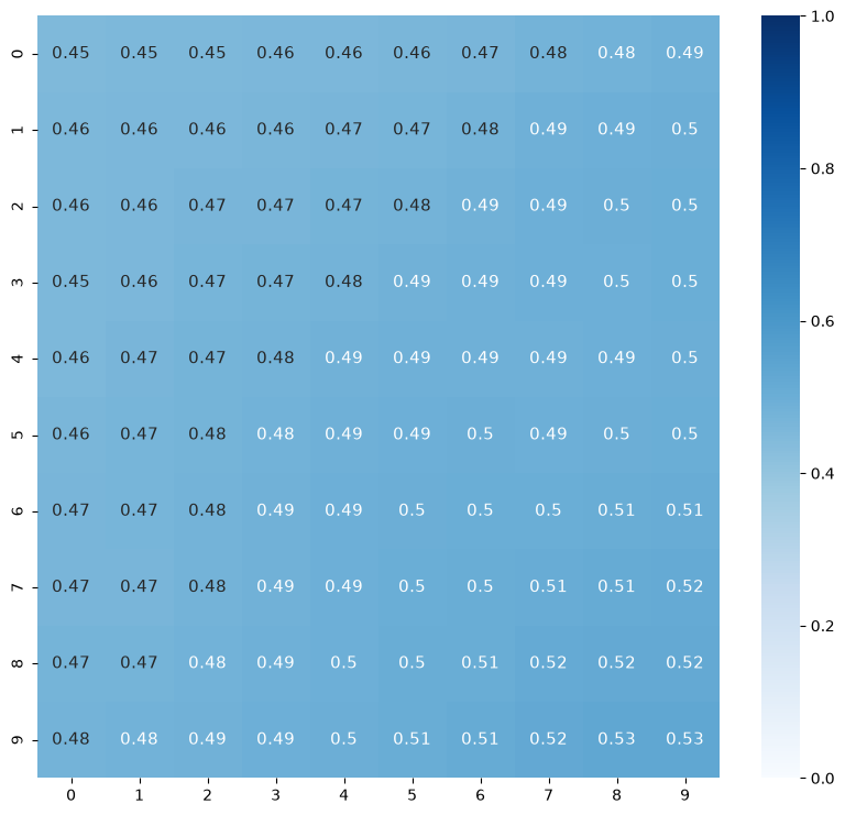

<Figure size 640x480 with 0 Axes>

Let’s check out a small section of the lightning strike data:

plt.figure(figsize=(6,5))
sns.heatmap(ds.lightning_flashes.isel(t=0)[3:9,3:9], 
            cmap="Blues", 
            annot=True, 
            annot_kws={"size": 11}) # font size

plt.show()
plt.tight_layout()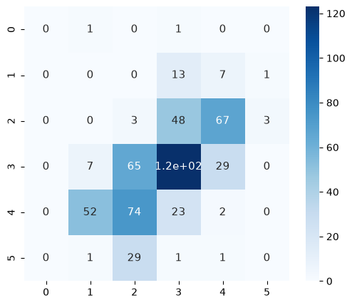

<Figure size 640x480 with 0 Axes>

After reviewing the dataset, some of the variables have different shapes:

print(ds.visible.shape) # x, y, time
print(ds.lightning_flashes.shape)

(768, 768, 12)
(48, 48, 12)

Using xESMF to regrid an xarray dataset:¶

Information available here: https://xesmf.readthedocs.io/en/latest/notebooks/Rectilinear_grid.html

In order to re-grid, let’s set up some coordinates. Lets do some sanity checking to check what the axises needs to be divided by:

# Why 47 and not 48? The range for x4 is 0 to 47 (48 steps). If you divide by 48, it will be longer by ~1 in each dimmension
np.shape(ds.visible.values)[0]/47 # for both x & y, this number does not need to be an integer

16.340425531914892

scaling_factor = np.shape(ds.lightning_flashes.values)

ds2 = ds.assign_coords(x4=ds.x4, y4=ds.y4, 
                        x=ds.x/16.3404, y=ds.y/16.340425, # make the coordinates match
                        time=ds.t) # making it a new dataset
ds2

Decreasing visible resoultion to lighting resoultion¶

Making new datasets, this might not be required.¶

ds_visible = ds2["visible"].to_dataset()
ds_visible = ds_visible.rename({'x': 'lon','y': 'lat'})
ds_visible

ds_lf = ds2["lightning_flashes"].to_dataset()
ds_lf = ds_lf.rename({'x4': 'lon',
                      'y4': 'lat'})
ds_lf

regridder = xe.Regridder(ds_visible, ds_lf, "bilinear")
regridder  # print basic regridder information.

xESMF Regridder 
Regridding algorithm:       bilinear 
Weight filename:            bilinear_768x768_48x48.nc 
Reuse pre-computed weights? False 
Input grid shape:           (768, 768) 
Output grid shape:          (48, 48) 
Periodic in longitude?      False

dr_out = regridder(ds_visible)
dr_out

Direct Comparison¶

Note the difference in x & y axis

time_step = 0

f, (ax1, ax2) = plt.subplots(1, 2, sharey=False, figsize=(8,8))
# Original figure
ax1.imshow(ds.visible.isel(t=time_step)[:,:]*1e-4,cmap='Greys_r',vmin=0,vmax=1) # the x and y axis were flipped, added the .T to fix the plot
ax1.title.set_text('Original')

ax2.imshow(dr_out.visible.isel(t=time_step)[:,:].T*1e-4,cmap='Greys_r',vmin=0,vmax=1) 
ax2.title.set_text('Downscaled - Bilinear')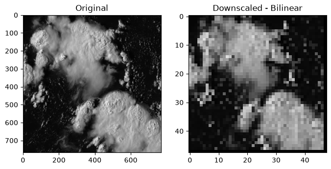

We can also upscale low-resoultion data¶

Note: This is not a reccomendation to do this for every workflow/dataset! There are five different algorithms that you can use, here is a nice comparison: https://xesmf.readthedocs.io/en/latest/notebooks/Compare_algorithms.html

regridder_up_con = xe.Regridder(ds_lf, ds_visible, "conservative") #note different method from before
regridder_up_patch = xe.Regridder(ds_lf, ds_visible, "patch") 
regridder_up_patch  # print basic regridder information.

xESMF Regridder 
Regridding algorithm:       patch 
Weight filename:            patch_48x48_768x768.nc 
Reuse pre-computed weights? False 
Input grid shape:           (48, 48) 
Output grid shape:          (768, 768) 
Periodic in longitude?      False

upscaled_lf_con = regridder_up_con(ds_lf)
upscaled_lf_patch = regridder_up_patch(ds_lf)

/home/runner/micromamba/envs/gridding-cookbook-dev/lib/python3.13/site-packages/xesmf/smm.py:131: UserWarning: Input array is not C_CONTIGUOUS. Will affect performance.
  warnings.warn('Input array is not C_CONTIGUOUS. ' 'Will affect performance.')
/home/runner/micromamba/envs/gridding-cookbook-dev/lib/python3.13/site-packages/xesmf/smm.py:131: UserWarning: Input array is not C_CONTIGUOUS. Will affect performance.
  warnings.warn('Input array is not C_CONTIGUOUS. ' 'Will affect performance.')

f, (ax1, ax2, ax3) = plt.subplots(1, 3, sharey=False, figsize=(10,4))

# Original Dataset
ax1.imshow(ds.lightning_flashes.isel(t=0)[:,:],cmap='GnBu')
ax1.title.set_text('Original')


ax2.imshow(upscaled_lf_con.lightning_flashes.isel(t=0)[:,:].T, cmap='GnBu')
ax2.title.set_text('Upscaled - Conservative')

ax3.imshow(upscaled_lf_patch.lightning_flashes.isel(t=0)[:,:].T, cmap='GnBu')
ax3.title.set_text('Upscaled - Patch')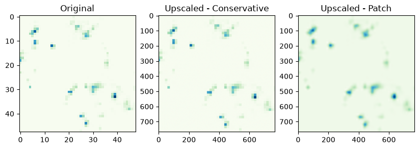

Merging Xarray Datasets¶

After you have made a new grid, you will want to combine them into a new xarray dataset for future analysis. Here is an example using combine by coords:

upscaled_lf_patch

ds_visible

new_dataset = xr.combine_by_coords([upscaled_lf_patch, ds_visible])
new_dataset

Summary¶

This has been a quick introduction to useing the xESMF regridding tools! The documentation for xESMF & xarray are very helpful for future learning.

Preamble

How to Cite This Cookbook

re(Gridding)

Introduction to Verde