Introduction to Verde - (re)Gridding with xarray

Unlike xESMF, verde is mainly designed around unstructured grids. Verde has a lot of great examples, we will use an atmospheric one below, but highly reccomend reading though the documents to get a better handle on the API.

https://www.fatiando.org/verde/latest/

Prerequisites¶

Knowing your way around pandas, xarray, numpy and matplotlib is beneficial. This is not deisgned to be an introduction to any of those packages. We will be using Cartopy for some of the plots as well.

Imports¶

import pandas as pd
import numpy as np
import cartopy.crs as ccrs
import cartopy.feature as cf

from appdirs import *

import verde as vd

import matplotlib.pyplot as plt
import matplotlib.ticker as mticker

%load_ext watermark
%watermark --iversions

appdirs   : 1.4.4
pandas    : 2.3.0
numpy     : 2.2.6
matplotlib: 3.10.3
cartopy   : 0.24.0
sys       : 3.13.5 | packaged by conda-forge | (main, Jun 16 2025, 08:27:50) [GCC 13.3.0]
verde     : 1.8.1

colnames=['remove', 'lon', 'lat', 'date', 'sensor', 'PM25value', 'sensor_type'] 

df = pd.read_csv('../data/airnow_data.csv', names=colnames, header=None)
df = df.drop(columns='remove')
df.head(3)

df.date = pd.to_datetime(df.date)
df.dtypes

lon                   float64
lat                   float64
date           datetime64[ns]
sensor                 object
PM25value               int64
sensor_type             int64
dtype: object

Let’s pick a time that has decent coverage:

df.date.value_counts().head()

date
2022-09-05 16:00:00    36
2022-09-05 17:00:00    36
2022-09-05 18:00:00    36
2022-09-05 19:00:00    36
2022-09-05 20:00:00    36
Name: count, dtype: int64

df2 = df[df.date == '2022-09-06T07:00']
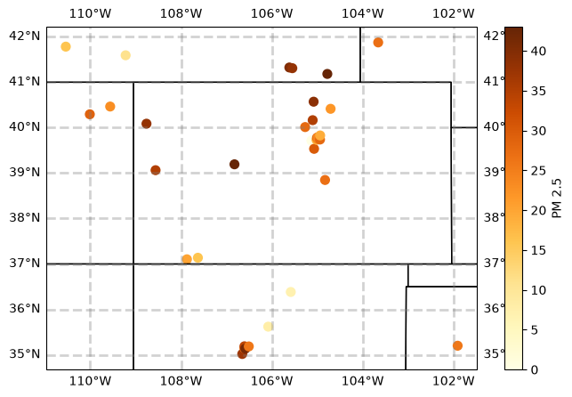
df2.head(3)

Plotting the data¶

plt.figure(figsize=(8, 5))
ax = plt.axes(projection=ccrs.PlateCarree())
ax.add_feature(cf.STATES)

gl = ax.gridlines(crs=ccrs.PlateCarree(), draw_labels=True,
                  linewidth=2, color='gray', alpha=0.35, linestyle='--')

gl.xlabels_top = False
gl.ylabels_right = False

gl.xlocator = mticker.FixedLocator([-110, -108,  -106, -104, -102])

plt.scatter(df2.lat, 
            df2.lon, 
            c = df2.PM25value,
            s=50,
            cmap="YlOrBr")

plt.colorbar().set_label("PM 2.5")
plt.show()

/home/runner/micromamba/envs/gridding-cookbook-dev/lib/python3.13/site-packages/cartopy/io/__init__.py:241: DownloadWarning: Downloading: https://naturalearth.s3.amazonaws.com/10m_cultural/ne_10m_admin_1_states_provinces_lakes.zip
  warnings.warn(f'Downloading: {url}', DownloadWarning)

Verde Workflows¶

Some of these workflows might not work super well from a scientific standpoint, this is just to show the mechanics of the verde package.

coordinates = (df2.lon, df2.lat)

Trend Estimation¶

Same code, different example can be found here: https://www.fatiando.org/verde/latest/tutorials/trends.html

trend = vd.Trend(degree=1).fit(coordinates, df2.PM25value)
print(trend.coef_)

[38.39163129  0.54379964  0.32281663]

trend_values = trend.predict(coordinates)
residuals = df2.PM25value - trend_values

plt.figure(figsize=(8, 5))
ax = plt.axes(projection=ccrs.PlateCarree())
ax.add_feature(cf.STATES)

gl = ax.gridlines(crs=ccrs.PlateCarree(), draw_labels=True,
                  linewidth=2, color='gray', alpha=0.35, linestyle='--')

gl.top_labels = False
gl.ylabels_right = False

gl.xlocator = mticker.FixedLocator([-110, -108,  -106, -104, -102])

maxabs = vd.maxabs(residuals)


plt.scatter(df2.lat, 
            df2.lon, 
            c = residuals,
            s=50,
            vmin=-maxabs,
            vmax=maxabs,
            cmap="bwr")

plt.colorbar().set_label("Residuals")
plt.show()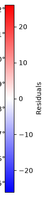

Unlike the Texas example in Verde, hard to see a distinct regional trend.

Data Decimation¶

spacing = 30 / 60 # Play around with this!

reducer = vd.BlockReduce(reduction=np.median, spacing= spacing)
print(reducer)

BlockReduce(reduction=<function median at 0x7f8ea04ca7f0>, spacing=0.5)

filter_coords, filter_data = reducer.filter(
    coordinates=(df2.lat, df2.lon), data=df2.PM25value)

/home/runner/micromamba/envs/gridding-cookbook-dev/lib/python3.13/site-packages/verde/blockreduce.py:179: FutureWarning: The provided callable <function median at 0x7f8ea04cfe20> is currently using DataFrameGroupBy.median. In a future version of pandas, the provided callable will be used directly. To keep current behavior pass the string "median" instead.
  blocked = pd.DataFrame(columns).groupby("block").aggregate(reduction)
/home/runner/micromamba/envs/gridding-cookbook-dev/lib/python3.13/site-packages/verde/blockreduce.py:236: FutureWarning: The provided callable <function median at 0x7f8ea04cfe20> is currently using DataFrameGroupBy.median. In a future version of pandas, the provided callable will be used directly. To keep current behavior pass the string "median" instead.
  grouped = table.groupby("block").aggregate(self.reduction)

Sanity check

np.shape(filter_coords)[1] == np.size(filter_data)

True

Plotting the decimated datapoints

plt.figure(figsize=(6, 4))
plt.plot(*filter_coords, ".k",  markersize=15, label='Data points')
plt.legend()
plt.show()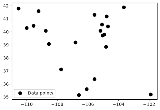

Verde Spline¶

This turtorial runs though this entire workflow, but with a bathymetery dataset: https://www.fatiando.org/verde/latest/tutorials/projections.html

spline = vd.Spline().fit(filter_coords, filter_data)

region = vd.get_region(filter_coords)
grid_coords = vd.grid_coordinates(region, spacing=spacing)
grid = spline.grid(coordinates=grid_coords, data_names="PM25")
print(grid)

<xarray.Dataset> Size: 2kB
Dimensions:   (northing: 14, easting: 18)
Coordinates:
  * easting   (easting) float64 144B -110.5 -110.0 -109.5 ... -102.4 -101.9
  * northing  (northing) float64 112B 35.14 35.66 36.18 ... 40.84 41.36 41.88
Data variables:
    PM25      (northing, easting) float64 2kB 74.69 69.09 63.62 ... 11.73 6.292
Attributes:
    metadata:  Generated by Spline(mindist=0)

distance_mask = 1 #this might not make physical sense
grid = vd.distance_mask(filter_coords, maxdist=distance_mask, grid=grid)

Let’s make a plot with the gridded and masked output, also shows where the datapoints are:

plt.figure(figsize=(8, 5))

pc = grid.PM25.plot.pcolormesh(cmap="YlOrBr", add_colorbar=False)
plt.colorbar(pc)
plt.plot(filter_coords[0], filter_coords[1], ".k", markersize=15, label='Data Points')

plt.title('Gridded PM2.5 Data, Distance Filter: '+str(distance_mask))

plt.xlabel("West", size=15)
plt.ylabel("North", size=15)
plt.legend()
plt.gca().set_aspect("equal")
plt.tight_layout()
plt.show()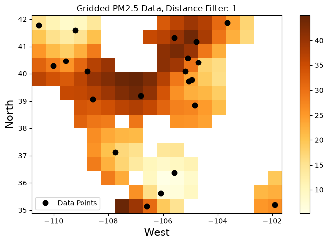

Xarray¶

Making the grid into an xarray dataset is 1 line of code!

ds = grid.PM25.to_dataset()
ds

Exporting this as a netCDF:

ds.to_netcdf('test.nc')

Summary¶

Verde and xESMF are two different gridding packages, with two different aims. They both work well with xarray!

re(Gridding)

xESMF Demo using SEVIER dataset for Machine Learning Preperation

re(Gridding)

Introduction to Pyresample