easy.gems for HEALPix Analysis & Visualization
In this section, you’ll learn:
Utilizing intake to open a HEALPix data catalog
Using the
healpixpackage to perform HEALPix operations to look at basic statisticsPlotting HEALPix data via easy.gems functionality
Related Documentation
Prerequisites
| Concepts | Importance | Notes |
|---|---|---|
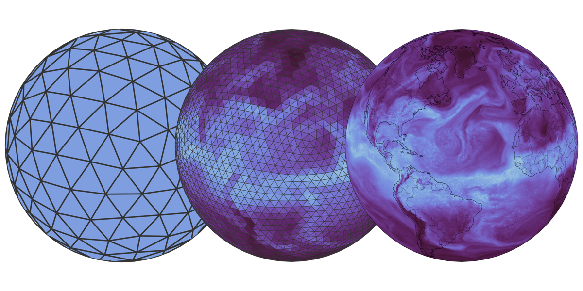
| HEALPix overview | Necessary |
Time to learn: 30 minutes
Open data catalog
Let us use the online data catalog from the WCRP’s Digital Earths Global Hackathon 2025’s catalog repository using intake and read the output of the ICON simulation run ngc4008, which is stored in the HEALPix format:
import intake

# Hackathon data catalogs
cat_url = "https://digital-earths-global-hackathon.github.io/catalog/catalog.yaml"
cat = intake.open_catalog(cat_url).online
model_run = cat.icon_ngc4008
/home/runner/micromamba/envs/healpix-cookbook-dev2/lib/python3.14/site-packages/intake/catalog/utils.py:173: UserWarning: Shell command not executed due to getshell=False
warnings.warn("Shell command not executed due to getshell=False")
/home/runner/micromamba/envs/healpix-cookbook-dev2/lib/python3.14/site-packages/intake/catalog/utils.py:182: UserWarning: Shell command not executed due to getshell=False
warnings.warn("Shell command not executed due to getshell=False")
Explore datasets
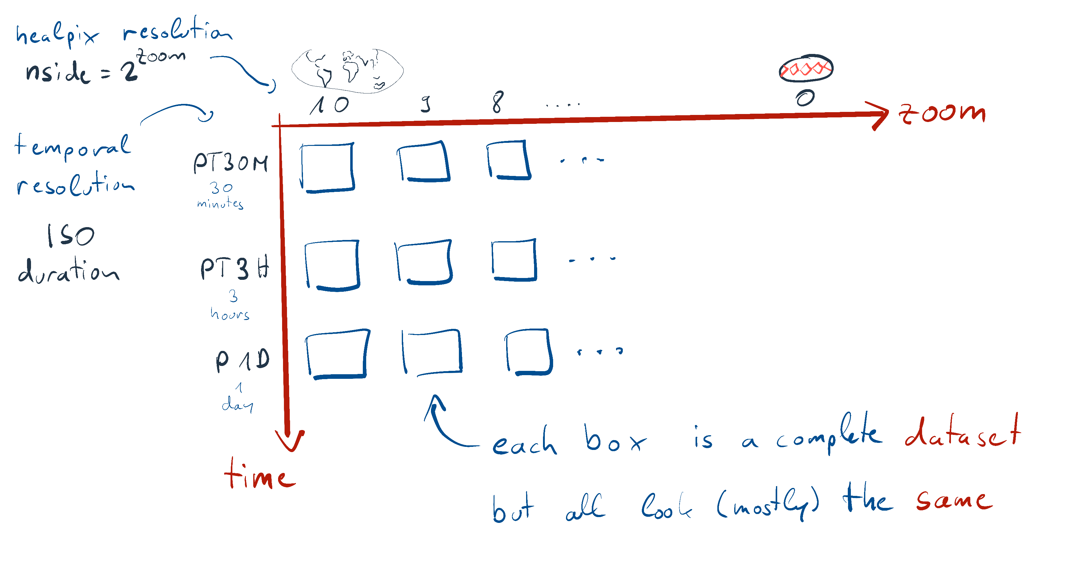
So, the coarsest dataset in this model run would be as follows (Even if we called it without specifying any parameters, i.e. model_run.to_dask(), the result would be same as the ds_coarsest below since this model run defaults to the coarsest settings):
ds_coarsest = model_run(zoom=0, time="P1D").to_dask()
ds_coarsestNow, let us look at a dataset with finer zoom level still with the coarsest time and another dataset with a finer zoom level and the finest time (which may be useful for daily analyses) dataset:
ds_fine = model_run(zoom=7).to_dask()
ds_fineds_finesttime = model_run(zoom=6, time="PT15M").to_dask()
ds_finesttimeHEALPix basic stats with thehealpix package
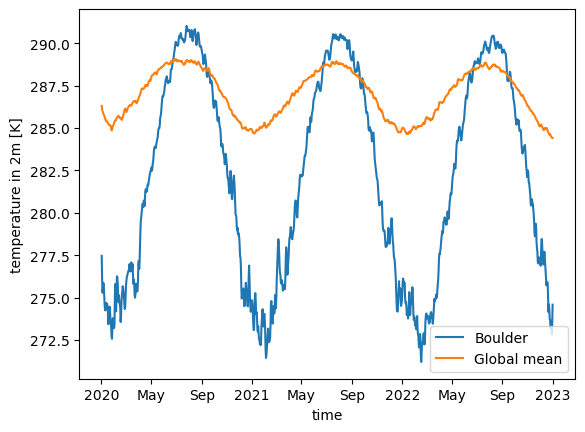
Let us look at the global and Boulder, CO, USA temperature averages for a 3-year time-slice of the whole dataset.
For this, we will first need to define a few HEALPix helper functions to get the nest and nside values from the dataset, then find the HEALPix pixel that Boulder coords fall in, and finally plot those temporal averages using matplotlib.
import healpix as hp
import matplotlib.pylab as plt
HEALPix helper functions
def get_nest(ds):
    return ds.crs.healpix_order == "nest"

def get_nside(ds):
    return ds.crs.healpix_nside

# The dataset used in this section uses the old easygems CRS convention.
# The new easygems (>=0.1.4) `guess_crs()` seems to be looking for these via
# `cf_xarray`'s grid mapping mechanism, which fails on the old data format
# So we will need to assign "crs" coords of the dataset properly
def fix_crs(ds):
    import xarray as xr

    crs_scalar = xr.DataArray(
        attrs={
            "grid_mapping_name": "healpix",
            "healpix_nside": get_nside(ds),
            "healpix_order": str(ds.crs.healpix_order),
        }
    )
    return ds.assign_coords(crs=crs_scalar)
HEALPix pixel containing Boulder’s coords
%%time
boulder_lon = -105.2747
boulder_lat = 40.0190

boulder_pixel = hp.ang2pix(
    get_nside(ds_fine), boulder_lon, boulder_lat, lonlat=True, nest=get_nest(ds_fine)
)
CPU times: user 368 μs, sys: 37 μs, total: 405 μs
Wall time: 412 μs
Global and Boulder’s temperature averages
%%time
time_slice = slice("2020-01-02T00:00:00.000000000", "2023-01-01T00:00:00.000000000")

ds_fine.tas.sel(time=time_slice).isel(cell=boulder_pixel).plot(label="Boulder")

ds_coarsest.tas.sel(time=time_slice).mean("cell").plot(label="Global mean")

plt.legend();
CPU times: user 42.5 ms, sys: 6.35 ms, total: 48.8 ms
Wall time: 1.8 s
Plotting with easy.gems and cartopy
In this part, we will look at the healpix_show function that is provided by easy.gems for convenient HEALPix plotting.
import easygems.healpix as eghp

import cartopy.crs as ccrs
import cartopy.feature as cf
import cmocean
/home/runner/micromamba/envs/healpix-cookbook-dev2/lib/python3.14/site-packages/tqdm/auto.py:21: TqdmWarning: IProgress not found. Please update jupyter and ipywidgets. See https://ipywidgets.readthedocs.io/en/stable/user_install.html
from .autonotebook import tqdm as notebook_tqdm
ds_fine = fix_crs(ds_fine)
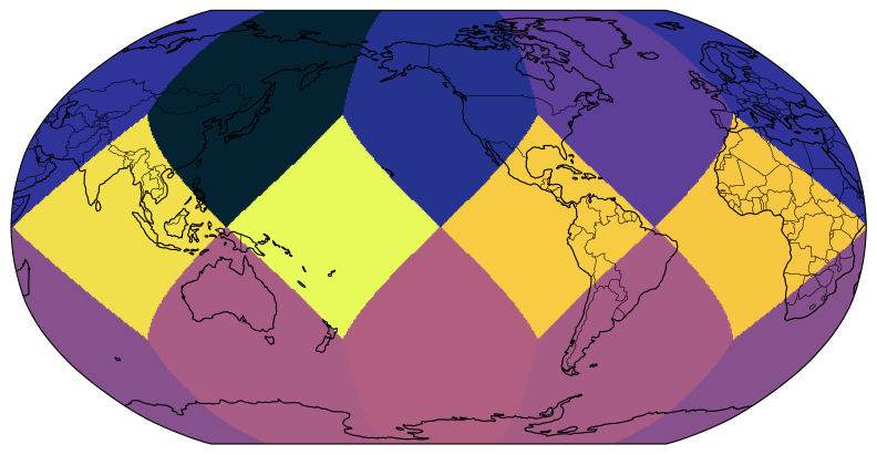
da_fine = ds_fine.tas.isel(time=0)Global plots
Most of this is matplotlib and cartopy code, but have a look at how eghp.healpix_show() is called. The following code will plot global temperature (at the first timestep for simplicity)
projection = ccrs.Robinson(central_longitude=-135.5808361)

fig, ax = plt.subplots(
    figsize=(8, 4), subplot_kw={"projection": projection}, constrained_layout=True
)

ax.set_global()

eghp.healpix_show(da_fine, ax=ax, cmap=cmocean.cm.thermal)

ax.add_feature(cf.COASTLINE, linewidth=0.8)
ax.add_feature(cf.BORDERS, linewidth=0.4);
/home/runner/micromamba/envs/healpix-cookbook-dev2/lib/python3.14/site-packages/cartopy/io/__init__.py:242: DownloadWarning: Downloading: https://naturalearth.s3.amazonaws.com/110m_physical/ne_110m_coastline.zip
warnings.warn(f'Downloading: {url}', DownloadWarning)
/home/runner/micromamba/envs/healpix-cookbook-dev2/lib/python3.14/site-packages/cartopy/io/__init__.py:242: DownloadWarning: Downloading: https://naturalearth.s3.amazonaws.com/110m_cultural/ne_110m_admin_0_boundary_lines_land.zip
  warnings.warn(f'Downloading: {url}', DownloadWarning)
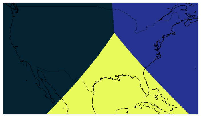
Regional plots
If plotting a region of interest is desired, it is also possible through setting extents of the matplotlib plot.
Let us look into USA map using the Boulder, CO, USA coords we had used before for simplicity:
projection = ccrs.Robinson(central_longitude=boulder_lon)

fig, ax = plt.subplots(
    figsize=(8, 4), subplot_kw={"projection": projection}, constrained_layout=True
)
ax.set_extent([boulder_lon-20, boulder_lon+40, boulder_lat-20, boulder_lat+10], crs=ccrs.PlateCarree())

eghp.healpix_show(da_fine, ax=ax, cmap=cmocean.cm.thermal)

ax.add_feature(cf.COASTLINE, linewidth=0.8)
ax.add_feature(cf.BORDERS, linewidth=0.4);
/home/runner/micromamba/envs/healpix-cookbook-dev2/lib/python3.14/site-packages/cartopy/io/__init__.py:242: DownloadWarning: Downloading: https://naturalearth.s3.amazonaws.com/50m_physical/ne_50m_coastline.zip
warnings.warn(f'Downloading: {url}', DownloadWarning)
/home/runner/micromamba/envs/healpix-cookbook-dev2/lib/python3.14/site-packages/cartopy/io/__init__.py:242: DownloadWarning: Downloading: https://naturalearth.s3.amazonaws.com/50m_cultural/ne_50m_admin_0_boundary_lines_land.zip
  warnings.warn(f'Downloading: {url}', DownloadWarning)
Further easy.gems and healpix
These are only a sampling of HEALPix and easy.gems capabilities; if you are interested in learning more, be sure to check out the usage examples at the easy.gems HEALPix Documentation.
What is next?
The next section will provide an UXarray workflow that loads in and analyzes & visualizes HEALPix data.