UXarray for Basic HEALPix Statistics & Visualization¶

In this section, you’ll learn:¶

Utilizing intake to open a HEALPix data catalog
Using the uxarray package to look at basic statistics over HEALPix data
Using UXarray plotting functionality on HEALPix data

Prerequisites¶

Concepts	Importance	Notes
UXarray	Necessary
HEALPix overview	Necessary

Time to learn: 30 minutes

import cartopy.crs as ccrs
import uxarray as ux

Open data catalog¶

Let us use the online data catalog from the WCRP’s Digital Earths Global Hackathon 2025’s catalog repository using intake and read the output of the ICON simulation run ngc4008, which is stored in the HEALPix format:

import intake

# Hackathon data catalogs
cat_url = "https://digital-earths-global-hackathon.github.io/catalog/catalog.yaml"
cat = intake.open_catalog(cat_url).online
model_run = cat.icon_ngc4008

/home/runner/micromamba/envs/healpix-cookbook-dev2/lib/python3.13/site-packages/intake/catalog/utils.py:173: UserWarning: Shell command not executed due to getshell=False
  warnings.warn("Shell command not executed due to getshell=False")
/home/runner/micromamba/envs/healpix-cookbook-dev2/lib/python3.13/site-packages/intake/catalog/utils.py:182: UserWarning: Shell command not executed due to getshell=False
  warnings.warn("Shell command not executed due to getshell=False")

We will be looking at two resolution levels, one is the coarsest zoom level of 0, which is the default in this model run, and the other is a finer one at the zoom level of 7:

ds_coarsest = model_run().to_dask()
ds_fine = model_run(zoom=7).to_dask()

Create UXarray Datasets from HEALPix¶

Now let us use those xarray.Datasets from the model run to open unstructured grid-aware uxarray.UxDataset:

%%time
uxds_coarsest = ux.UxDataset.from_healpix(ds_coarsest)

uxds_fine = ux.UxDataset.from_healpix(ds_fine)
uxds_fine

CPU times: user 22.6 ms, sys: 1.92 ms, total: 24.5 ms
Wall time: 23.6 ms

HEALPix basic stats using UXarray¶

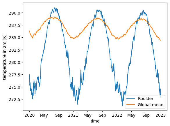
Let us look at the global and Boulder, CO, USA air temperature averages for the dataset. Data spans from 2020 to 2050, so let us also consider slicing it to have a 3-year interval between 2020 and 2023, which would also give us similar results to that with easy.gems in the previous section.

import matplotlib.pylab as plt

boulder_lon = -105.2747
boulder_lat = 40.0190

time_slice = slice("2020-01-02T00:00:00.000000000", "2023-01-01T00:00:00.000000000")

Mesh face containing Boulder’s coords¶

We can find face(s) containing a given point with uxarray conveniently as follows:

%%time
boulder_face = uxds_fine.uxgrid.get_faces_containing_point(
    points=[boulder_lon, boulder_lat],
    return_counts=False
)[0]
boulder_face

CPU times: user 8.97 s, sys: 916 ms, total: 9.89 s
Wall time: 9.89 s

[2]

Data variables of interest¶

In order to use in the rest of the analyses, we can grab data variables, in theuxarray.UxDataArray type, from the dataset as follows:

uxda_fine = uxds_fine.tas
uxda_coarsest = uxds_coarsest.tas

Global and Boulder’s temperature averages¶

In order to get a line plot of our UXarray.UxDataset objects’ 1-dimensional temperature variables, we will convert them to xarray and call the default plot function because UXarray’s default plotting functions are all dedicated to grid-topology aware visualizations:

uxda_fine.isel(n_face=boulder_face)

%%time
uxda_fine.isel(n_face=boulder_face).sel(time=time_slice).to_xarray().plot(
    label="Boulder"
)
uxda_coarsest.sel(time=time_slice).mean("n_face").to_xarray().plot(label="Global mean")

plt.legend()

CPU times: user 30.9 ms, sys: 6.83 ms, total: 37.7 ms
Wall time: 1.17 s

Data plotting with UXarray¶

UXarray provides several built-in plotting functions to visualize unstructured grids, which can also be applied to HEALPix grids in the same interface:

Let us first look into interactive plots with the bokeh backend (i.e. UXarray’s plotting functions have a backend parameter that defaults to “bokeh”, and it can also accept “matplotlib”)

Global plots¶

Let us first plot the global temperature (at the first timestep for simplicity), using the default backend, bokeh, of UXarray’s visualization API to create an interactive plot:

%%time

projection = ccrs.Robinson(central_longitude=-135.5808361)

uxda_fine.isel(time=0).plot(
    projection=projection,
    cmap="inferno",
    features=["borders", "coastline"],
    title="Global temperature",
    width=700,
)

CPU times: user 3.08 s, sys: 210 ms, total: 3.29 s
Wall time: 3.83 s

WARNING:param.GeoOverlayPlot00481: Due to internal constraints, when aspect and width/height is set, the bokeh backend uses those values as frame_width/frame_height instead. This ensures the aspect is respected, but means that the plot might be slightly larger than anticipated. Set the frame_width/frame_height explicitly to suppress this warning.

Now, let us create the same plot, using matplotlib as the backend:

%%time

uxda_fine.isel(time=0).plot(
    backend="matplotlib",
    projection=projection,
    cmap="inferno",
    features=["borders", "coastline"],
    title="Global temperature",
    width=1100,
)

CPU times: user 481 ms, sys: 11.2 ms, total: 492 ms
Wall time: 1 s

Regional subsets (Not only for plotting but also for analysis)¶

When a region on the globe is of interest, UXarray provides subsetting functions, which return new regional grids that can then be used in the same way a global grid is plotted.

Let us look into the USA map using the Boulder, CO, USA coords we had used before for simplicity:

Subsetting uxds_fine into a new UxDataset using a “bounding box” around Boulder, CO first:

%%time

lon_bounds = (boulder_lon - 20, boulder_lon + 40)
lat_bounds = (boulder_lat - 20, boulder_lat + 12)

uxda_fine_subset = uxda_fine.isel(time=0).subset.bounding_box(lon_bounds, lat_bounds)

CPU times: user 15.3 s, sys: 711 ms, total: 16 s
Wall time: 16 s

If we check the global and regional subset’s average temperature at the first timestep, we can see the difference:

print(
    "Global temperature average: ", uxda_fine.isel(time=0).mean("n_face").values, " K"
)
print(
    "Regional subset's temperature average: ", uxda_fine_subset.mean("n_face").values, " K"
)

Global temperature average:  286.30957  K
Regional subset's temperature average:  nan  K

Now, let us plot the regional subset UxDataset:

%%time
projection = ccrs.Robinson(central_longitude=boulder_lon)

uxda_fine_subset.plot(
    projection=projection,
    cmap="inferno",
    features=["borders", "coastline"],
    title="Boulder temperature",
    width=1100,
)

CPU times: user 39.4 ms, sys: 2.95 ms, total: 42.3 ms
Wall time: 41.4 ms

Grid topology exploration¶

Exploring the grid topology may be needed sometimes, and UXarray provides functionality to do so, both numerically and visually. Each UxDataset or UxDataArray has their associated Grid object that has all the information such as spherical and cartesian coordinates, connectives, dimensions, etc. about the topology this data belongs to. This Grid object can be explored as follows:

# uxds_fine.uxgrid   # this would give the same as the below
uxda_fine.uxgrid

There might be times that the user wants to open a standalone Grid object for a HEALPix grid (or any other unstructured grids supported by UXarray) without accessing the data yet. Let’s create the coarsest HEALPix grid as follows:

uxgrid = ux.Grid.from_healpix(zoom=0, pixels_only=False)
uxgrid

Let’s investigate how a HEALPix grid looks like over the poles. We can do things by selecting an Orthographic projection and setting a Geodetic source projection. This allows to better approximates the true HEALPix structured compared to the defaut PlateCaree projection.

projection = ccrs.Orthographic(central_latitude=90)
projection.threshold /= 100  # Smoothes out great circle arcs

uxgrid.plot(
    periodic_elements="ignore",  # Allow Cartopy to handle periodic elements
    crs=ccrs.Geodetic(),  # Enables edges to be plotted as GCAs
    project=True,
    projection=projection,
    width=500,
    title="HEALPix (Orthographic Proj), zoom=0",
)

Let’s chose another projection.

projection = ccrs.Mollweide()
projection.threshold /= 100  # Smoothes out great circle arcs

uxgrid.plot(
    periodic_elements="ignore",  # Allow Cartopy to handle periodic elements
    crs=ccrs.Geodetic(),  # Enables edges to be plotted as GCAs
    project=True,
    projection=projection,
    width=500,
    title="HEALPix (Mollweide Proj), zoom=0",
)

The grid structure here is approximated. While the boundary between each pixel is easily known in HEALPix workflows, UXarray represents the boundaries as a Great Circle Arc (GCA) due to the requirement of having explicit connectivity information, which is different than HEALPix boundaries and leads to minor differences in the computed plots and computations.

Now that we’ve looked at the grid structure, we can also apply the same principles to our data plotting.

uxda_coarsest.isel(time=0).plot(
    periodic_elements="ignore",  # Allow Cartopy to handle periodic elements
    crs=ccrs.Geodetic(),  # Enables edges to be plotted as GCAs
    project=True,
    projection=projection,
    features=["borders", "coastline"],
    cmap="inferno",
    title="Temperature (Mollweide Proj), zoom=0",
    width=500,
)

What is next?¶

The next section will provide an UXarray workflow that loads in and analyzes & visualizes HEALPix data.

UXarray for Basic HEALPix Statistics & Visualization

UXarray for Basic HEALPix Statistics & Visualization¶

In this section, you’ll learn:¶

Related Documentation¶

Prerequisites¶

Open data catalog¶

Create UXarray Datasets from HEALPix¶

HEALPix basic stats using UXarray¶

Mesh face containing Boulder’s coords¶

Data variables of interest¶

Global and Boulder’s temperature averages¶

Data plotting with UXarray¶

Global plots¶

Regional subsets (Not only for plotting but also for analysis)¶

Grid topology exploration¶

What is next?¶