Kerchunk, GeoTIFF and Generating Coordinates with xrefcoord
Overview
In this tutorial we will cover:
How to generate
Kerchunkreferences of GeoTIFFs.Combining
Kerchunkreferences into a virtual dataset.Generating Coordinates with the
xrefcoordaccessor.
Prerequisites
Concepts |
Importance |
Notes |
|---|---|---|
Required |
Core |
|
Required |
Core |
|
Required |
Core |
|
Required |
IO/Visualization |
Time to learn: 30 minutes
About the Dataset
The Finish Meterological Institute (FMI) Weather Radar Dataset is a collection of GeoTIFF files containing multiple radar specific variables, such as rainfall intensity, precipitation accumulation (in 1, 12 and 24 hour increments), radar reflectivity, radial velocity, rain classification and the cloud top height. It is available through the AWS public data portal and is updated frequently.
More details on this dataset can be found here.
import glob
import logging
from tempfile import TemporaryDirectory

import dask
import fsspec
import numpy as np
import pandas as pd
import rioxarray
import s3fs
import ujson
import xarray as xr
import xrefcoord  # noqa
from distributed import Client
from kerchunk.combine import MultiZarrToZarr
from kerchunk.tiff import tiff_to_zarr
from tqdm import tqdm
Examining a Single GeoTIFF File
Before we use Kerchunk to create indices for multiple files, we can load a single GeoTiff file to examine it.
# URL pointing to a single GeoTIFF file
url = "s3://fmi-opendata-radar-geotiff/2023/07/01/FIN-ACRR-3067-1KM/202307010100_FIN-ACRR1H-3067-1KM.tif"

# Initialize a s3 filesystem
fs = s3fs.S3FileSystem(anon=True)

xds = rioxarray.open_rasterio(fs.open(url))
xds
<xarray.DataArray (band: 1, y: 1345, x: 850)>
[1143250 values with dtype=uint16]
Coordinates:
  * band         (band) int64 1
  * x            (x) float64 -1.177e+05 -1.166e+05 ... 8.738e+05 8.75e+05
  * y            (y) float64 7.907e+06 7.906e+06 ... 6.337e+06 6.336e+06
    spatial_ref  int64 0
Attributes:
    AREA_OR_POINT:  Area
    GDAL_METADATA:  <GDALMetadata>\n<Item name="Observation time" format="YYY...
    scale_factor:   1.0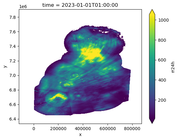
add_offset: 0.0xds.isel(band=0).where(xds < 2000).plot()
<matplotlib.collections.QuadMesh at 0x7f7f05fe8a60>
Create Input File List
Here we are using fsspec's glob functionality along with the * wildcard operator and some string slicing to grab a list of GeoTIFF files from a s3 fsspec filesystem.
# Initiate fsspec filesystems for reading
fs_read = fsspec.filesystem("s3", anon=True, skip_instance_cache=True)

files_paths = fs_read.glob(
    "s3://fmi-opendata-radar-geotiff/2023/01/01/FIN-ACRR-3067-1KM/*24H-3067-1KM.tif"
)
# Here we prepend the prefix 's3://', which points to AWS.
file_pattern = sorted(["s3://" + f for f in files_paths])
# This dictionary will be passed as kwargs to `fsspec`. For more details, check out the `foundations/kerchunk_basics` notebook.
so = dict(mode="rb", anon=True, default_fill_cache=False, default_cache_type="first")

# We are creating a temporary directory to store the .json reference files
# Alternately, you could write these to cloud storage.
td = TemporaryDirectory()
temp_dir = td.name
temp_dir
'/tmp/tmp3v5l212j'
Start a Dask Client
To parallelize the creation of our reference files, we will use Dask. For a detailed guide on how to use Dask and Kerchunk, see the Foundations notebook: Kerchunk and Dask.
client = Client(n_workers=8, silence_logs=logging.ERROR)
client
Client
Client-26ea85fc-21bd-11ee-8e7d-0022481ea464
| Connection method: Cluster object | Cluster type: distributed.LocalCluster |
| Dashboard: http://127.0.0.1:8787/status |
Cluster Info
LocalCluster
36ffec7e
| Dashboard: http://127.0.0.1:8787/status | Workers: 8 |
| Total threads: 8 | Total memory: 6.77 GiB |
| Status: running | Using processes: True |
Scheduler Info
Scheduler
Scheduler-213775d5-035e-4e84-9da9-0142c968105a
| Comm: tcp://127.0.0.1:34877 | Workers: 8 |
| Dashboard: http://127.0.0.1:8787/status | Total threads: 8 |
| Started: Just now | Total memory: 6.77 GiB |
Workers
Worker: 0
| Comm: tcp://127.0.0.1:38985 | Total threads: 1 |
| Dashboard: http://127.0.0.1:33203/status | Memory: 866.49 MiB |
| Nanny: tcp://127.0.0.1:39639 | |
| Local directory: /tmp/dask-scratch-space/worker-tg28vkzb | |
Worker: 1
| Comm: tcp://127.0.0.1:37423 | Total threads: 1 |
| Dashboard: http://127.0.0.1:39079/status | Memory: 866.49 MiB |
| Nanny: tcp://127.0.0.1:42551 | |
| Local directory: /tmp/dask-scratch-space/worker-8as53sld | |
Worker: 2
| Comm: tcp://127.0.0.1:43091 | Total threads: 1 |
| Dashboard: http://127.0.0.1:35709/status | Memory: 866.49 MiB |
| Nanny: tcp://127.0.0.1:44339 | |
| Local directory: /tmp/dask-scratch-space/worker-nyudetmg | |
Worker: 3
| Comm: tcp://127.0.0.1:43383 | Total threads: 1 |
| Dashboard: http://127.0.0.1:44549/status | Memory: 866.49 MiB |
| Nanny: tcp://127.0.0.1:37833 | |
| Local directory: /tmp/dask-scratch-space/worker-ceuz79j2 | |
Worker: 4
| Comm: tcp://127.0.0.1:45665 | Total threads: 1 |
| Dashboard: http://127.0.0.1:43553/status | Memory: 866.49 MiB |
| Nanny: tcp://127.0.0.1:43767 | |
| Local directory: /tmp/dask-scratch-space/worker-kegnjjtd | |
Worker: 5
| Comm: tcp://127.0.0.1:35233 | Total threads: 1 |
| Dashboard: http://127.0.0.1:36071/status | Memory: 866.49 MiB |
| Nanny: tcp://127.0.0.1:39955 | |
| Local directory: /tmp/dask-scratch-space/worker-zeh8djxm | |
Worker: 6
| Comm: tcp://127.0.0.1:39065 | Total threads: 1 |
| Dashboard: http://127.0.0.1:41511/status | Memory: 866.49 MiB |
| Nanny: tcp://127.0.0.1:39119 | |
| Local directory: /tmp/dask-scratch-space/worker-oo1bt3_e | |
Worker: 7
| Comm: tcp://127.0.0.1:44915 | Total threads: 1 |
| Dashboard: http://127.0.0.1:37353/status | Memory: 866.49 MiB |
| Nanny: tcp://127.0.0.1:42621 | |
| Local directory: /tmp/dask-scratch-space/worker-bh8s6s97 | |
# Use Kerchunk's `tiff_to_zarr` method to create create reference files


def generate_json_reference(fil, output_dir: str):
    tiff_chunks = tiff_to_zarr(fil, remote_options={"protocol": "s3", "anon": True})
    fname = fil.split("/")[-1].split("_")[0]
    outf = f"{output_dir}/{fname}.json"
    with open(outf, "wb") as f:
        f.write(ujson.dumps(tiff_chunks).encode())
    return outf


# Generate Dask Delayed objects
tasks = [dask.delayed(generate_json_reference)(fil, temp_dir) for fil in file_pattern]
# Start parallel processing
import warnings

warnings.filterwarnings("ignore")
dask.compute(tasks)
(['/tmp/tmp3v5l212j/202301010100.json',
  '/tmp/tmp3v5l212j/202301010200.json',
  '/tmp/tmp3v5l212j/202301010300.json',
  '/tmp/tmp3v5l212j/202301010400.json',
  '/tmp/tmp3v5l212j/202301010500.json',
  '/tmp/tmp3v5l212j/202301010600.json',
  '/tmp/tmp3v5l212j/202301010700.json',
  '/tmp/tmp3v5l212j/202301010800.json',
  '/tmp/tmp3v5l212j/202301010900.json',
  '/tmp/tmp3v5l212j/202301011000.json',
  '/tmp/tmp3v5l212j/202301011100.json',
  '/tmp/tmp3v5l212j/202301011200.json',
  '/tmp/tmp3v5l212j/202301011300.json',
  '/tmp/tmp3v5l212j/202301011400.json',
  '/tmp/tmp3v5l212j/202301011500.json',
  '/tmp/tmp3v5l212j/202301011600.json',
  '/tmp/tmp3v5l212j/202301011700.json',
  '/tmp/tmp3v5l212j/202301011800.json',
  '/tmp/tmp3v5l212j/202301011900.json',
  '/tmp/tmp3v5l212j/202301012000.json',
  '/tmp/tmp3v5l212j/202301012100.json',
  '/tmp/tmp3v5l212j/202301012200.json',
  '/tmp/tmp3v5l212j/202301012300.json'],)
Combine Reference Files into Multi-File Reference Dataset
Now we will combine all the reference files generated into a single reference dataset. Since each TIFF file is a single timeslice and the only temporal information is stored in the filepath, we will have to specify the coo_map kwarg in MultiZarrToZarr to build a dimension from the filepath attributes.
ref_files = sorted(glob.iglob(f"{temp_dir}/*.json"))


# Custom Kerchunk function from `coo_map` to create dimensions
def fn_to_time(index, fs, var, fn):
    import datetime
    import re

    subst = fn.split("/")[-1].split(".json")[0]
    return datetime.datetime.strptime(subst, "%Y%m%d%H%M")


mzz = MultiZarrToZarr(
    path=ref_files,
    indicts=ref_files,
    remote_protocol="s3",
    remote_options={"anon": True},
    coo_map={"time": fn_to_time},
    coo_dtypes={"time": np.dtype("M8[s]")},
    concat_dims=["time"],
    identical_dims=["X", "Y"],
)

# # save translate reference in memory for later visualization
multi_kerchunk = mzz.translate()

# Write kerchunk .json record
output_fname = "RADAR.json"
with open(f"{output_fname}", "wb") as f:
    f.write(ujson.dumps(multi_kerchunk).encode())
Open Combined Reference Dataset
fs = fsspec.filesystem(
    "reference",
    fo="RADAR.json",
    remote_protocol="s3",
    remote_options={"anon": True},
    skip_instance_cache=True,
)
m = fs.get_mapper("")
ds = xr.open_dataset(m, engine="zarr")
ds
<xarray.Dataset>
Dimensions: (time: 23, Y: 1345, X: 850, Y1: 673, X1: 425, Y2: 337, X2: 213,
Y3: 169, X3: 107, Y4: 85, X4: 54, Y5: 43, X5: 27)
Coordinates:
* time (time) datetime64[s] 2023-01-01T01:00:00 ... 2023-01-01T23:00:00
Dimensions without coordinates: Y, X, Y1, X1, Y2, X2, Y3, X3, Y4, X4, Y5, X5
Data variables:
0 (time, Y, X) float32 ...
1 (time, Y1, X1) float32 ...
2 (time, Y2, X2) float32 ...
3 (time, Y3, X3) float32 ...
4 (time, Y4, X4) float32 ...
5 (time, Y5, X5) float32 ...
Attributes: (12/15)
multiscales: [{'datasets': [{'path': '0'}, {'path': '1'}, {'p...
GDAL_METADATA: <GDALMetadata>\n<Item name="Observ...
KeyDirectoryVersion: 1
KeyRevision: 1
KeyRevisionMinor: 0
GTModelTypeGeoKey: 1
... ...
GeogAngularUnitsGeoKey: 9102
GeogTOWGS84GeoKey: [0.0, 0.0, 0.0]
ProjectedCSTypeGeoKey: 3067
ProjLinearUnitsGeoKey: 9001
ModelPixelScale: [1169.2930568410832, 1168.8701637541064, 0.0]
ModelTiepoint: [0.0, 0.0, 0.0, -118331.36640835612, 7907751.537...Use xrefcoord to Generate Coordinates
When using Kerchunk to generate reference datasets for GeoTIFF’s, only the dimensions are preserved. xrefcoord is a small utility that allows us to generate coordinates for these reference datasets using the geospatial metadata. Similar to other accessor add-on libraries for Xarray such as rioxarray and xwrf, xrefcord provides an accessor for an Xarray dataset. Importing xrefcoord allows us to use the .xref accessor to access additional methods.
In the following cell, we will use the generate_coords method to build coordinates for the Xarray dataset. xrefcoord is very experimental and makes assumptions about the underlying data, such as each variable shares the same dimensions etc. Use with caution!
# Generate coordinates from reference dataset
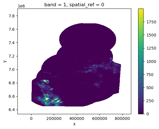
ref_ds = ds.xref.generate_coords(time_dim_name="time", x_dim_name="X", y_dim_name="Y")
# Rename to rain accumulation in 24 hour period
ref_ds = ref_ds.rename({"0": "rr24h"})