Smoothing Contours

Demonstrate how to smooth contour values from a higher resolution model field.

By: Kevin Goebbert

Date: 13 April 2017

Do the needed imports

from datetime import datetime

import cartopy.crs as ccrs
import cartopy.feature as cfeature
import matplotlib.pyplot as plt
import metpy.calc as mpcalc
import numpy as np
from metpy.units import units
from siphon.catalog import TDSCatalog
from xarray.backends import NetCDF4DataStore
import xarray as xr

Set up netCDF Subset Service link

# Specify our date/time of product desired
dt = datetime.utcnow()

# Construct the URL for our THREDDS Data Server Catalog,
# and access our desired dataset within via NCSS
cat = TDSCatalog('https://thredds.ucar.edu/thredds/catalog/grib/'
                 'NCEP/NAM/CONUS_12km/latest.xml')
ncss = cat.datasets[0].subset()

# Create our NCSS query with desired specifications
query = ncss.query()
query.time(dt)
query.add_lonlat()
query.variables('Geopotential_height_isobaric',
                'u-component_of_wind_isobaric',
                'v-component_of_wind_isobaric')

# Obtain the data we've queried for
data = ncss.get_data(query)

# Make into an xarray Dataset object
ds = xr.open_dataset(NetCDF4DataStore(data)).metpy.parse_cf()

Pull apart the data

# Get dimension names to pull appropriate variables
# dtime = ds.Geopotential_height_isobaric.dims[0]
# dlev = ds.Geopotential_height_isobaric.dims[1]
# dlat = ds.Geopotential_height_isobaric.dims[2]
# dlon = ds.Geopotential_height_isobaric.dims[3]

# Get lat and lon data, as well as time data and metadata
lats = ds.lat
lons = ds.lon

# Need 2D lat/lons for plotting, do so if necessary
if lats.ndim < 2:
    lons, lats = np.meshgrid(lons, lats)

# Determine the level of 500 hPa
lev_500 = 500 * units.hPa

# Create more useable times for output
times = ds.Geopotential_height_isobaric.metpy.time.squeeze()
vtimes = times.values.astype('datetime64[ms]').astype('O')

# Pull out the 500 hPa Heights
hght_500 = ds.Geopotential_height_isobaric.metpy.sel(
    vertical=lev_500).squeeze()
uwnd_500 = ds['u-component_of_wind_isobaric'].metpy.sel(
    vertical=lev_500).squeeze()
vwnd_500 = ds['v-component_of_wind_isobaric'].metpy.sel(
    vertical=lev_500).squeeze()

# Calculate the magnitude of the wind speed in kts
sped = mpcalc.wind_speed(uwnd_500, vwnd_500).metpy.convert_units('knots')

Set up the projection for LCC

plotcrs = ccrs.LambertConformal(central_longitude=-100.0,
                                central_latitude=45.0)
datacrs = ccrs.PlateCarree(central_longitude=0.)

Subset and smooth

# Smooth the 500-hPa geopotential height field
# Be sure to only smooth the 2D field
Z_500 = mpcalc.smooth_gaussian(hght_500, 50)

Plot the contours

# Start plot with new figure and axis
fig = plt.figure(figsize=(17., 11.))
ax = plt.subplot(1, 1, 1, projection=plotcrs)

# Add some titles to make the plot readable by someone else
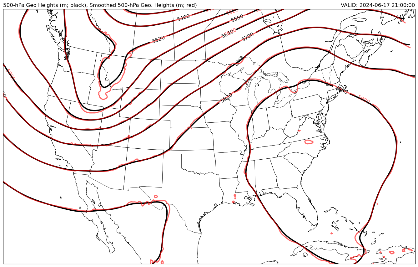
plt.title('500-hPa Geo Heights (m; black), Smoothed 500-hPa Geo. '
          'Heights (m; red)', loc='left')
plt.title(f'VALID: {vtimes}', loc='right')

# Set GAREA and add map features
ax.set_extent([-125., -67., 22., 52.], ccrs.PlateCarree())
ax.coastlines('50m', edgecolor='black', linewidth=0.75)
ax.add_feature(cfeature.STATES, linewidth=0.5)

# Set the CINT
clev500 = np.arange(5100, 6000, 60)

# Plot smoothed 500-hPa contours
cs2 = ax.contour(lons, lats, Z_500, clev500, colors='black',
                 linewidths=3, linestyles='solid', transform=datacrs)
c2 = plt.clabel(cs2, fontsize=12, colors='black', inline=1, inline_spacing=8,
                fmt='%i', rightside_up=True, use_clabeltext=True)

# Contour the 500 hPa heights with labels
cs = ax.contour(lons, lats, hght_500, clev500, colors='red',
                linewidths=2.5, linestyles='solid', alpha=0.6,
                transform=datacrs)
cl = plt.clabel(cs, fontsize=12, colors='red', inline=1, inline_spacing=8,
                fmt='%i', rightside_up=True, use_clabeltext=True)