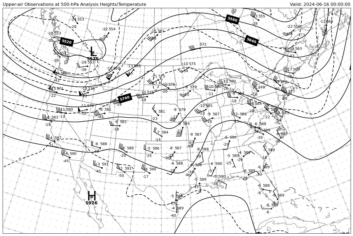
DIFAX Replication
This example replicates the traditional DIFAX images for upper-level observations.
By: Kevin Goebbert
Observation data comes from Iowa State Archive, accessed through the Siphon package. Contour data comes from the GFS 0.5 degree analysis. Classic upper-level data of Geopotential Height and Temperature are plotted.
import urllib.request

from datetime import datetime, timedelta

import cartopy.crs as ccrs
import cartopy.feature as cfeature
import matplotlib.pyplot as plt
from matplotlib.ticker import FixedLocator
import metpy.calc as mpcalc
import numpy as np
import xarray as xr

from metpy.io import add_station_lat_lon
from metpy.plots import StationPlot
from metpy.units import units
from siphon.simplewebservice.iastate import IAStateUpperAir
Plotting High/Low Symbols
A helper function to plot a text symbol (e.g., H, L) for relative maximum/minimum for a given field (e.g., geopotential height).
def plot_maxmin_points(lon, lat, data, extrema, nsize, symbol, color='k',
                       plotValue=True, transform=None):
    """
    This function will find and plot relative maximum and minimum for a 2D grid. The function
    can be used to plot an H for maximum values (e.g., High pressure) and an L for minimum
    values (e.g., low pressue). It is best to used filetered data to obtain  a synoptic scale
    max/min value. The symbol text can be set to a string value and optionally the color of the
    symbol and any plotted value can be set with the parameter color.

    Parameters
    ----------
        lon : 2D array
            Plotting longitude values
        lat : 2D array
            Plotting latitude values
        data : 2D array
            Data that you wish to plot the max/min symbol placement
        extrema : str
            Either a value of max for Maximum Values or min for Minimum Values
        nsize : int
            Size of the grid box to filter the max and min values to plot a reasonable number
        symbol : str
            Text to be placed at location of max/min value
        color : str
            Name of matplotlib colorname to plot the symbol (and numerical value, if plotted)
        plot_value : Boolean (True/False)
            Whether to plot the numeric value of max/min point

    Return
    ------
        The max/min symbol will be plotted on the current axes within the bounding frame
        (e.g., clip_on=True)
    """
    from scipy.ndimage import maximum_filter, minimum_filter

    if (extrema == 'max'):
        data_ext = maximum_filter(data, nsize, mode='nearest')
    elif (extrema == 'min'):
        data_ext = minimum_filter(data, nsize, mode='nearest')
    else:
        raise ValueError('Value for hilo must be either max or min')

    if lon.ndim == 1:
        lon, lat = np.meshgrid(lon, lat)

    mxx, mxy = np.where(data_ext == data)

    for i in range(len(mxy)):
        ax.text(lon[mxx[i], mxy[i]], lat[mxx[i], mxy[i]], symbol, color=color, size=36,
                clip_on=True, horizontalalignment='center', verticalalignment='center',
                transform=transform)
        ax.text(lon[mxx[i], mxy[i]], lat[mxx[i], mxy[i]],
                '\n' + str(np.int64(data[mxx[i], mxy[i]])),
                color=color, size=12, clip_on=True, fontweight='bold',
                horizontalalignment='center', verticalalignment='top', transform=transform)
        ax.plot(lon[mxx[i], mxy[i]], lat[mxx[i], mxy[i]], marker='o', markeredgecolor='black',
                markerfacecolor='white', transform=transform)
        ax.plot(lon[mxx[i], mxy[i]], lat[mxx[i], mxy[i]],
                marker='x', color='black', transform=transform)
Observation Data
Set a date and time for upper-air observations (should only be 00 or 12 UTC for the hour).
Request all data from Iowa State using the Siphon package. The result is a pandas DataFrame containing all of the sounding data from all available stations.
# Set date for desired UPA data
today = datetime.utcnow()

# Go back one day to ensure data availability
date = datetime(today.year, today.month, today.day, 0) - timedelta(days=1)

# Request data using Siphon request for data from Iowa State Archive
data = IAStateUpperAir.request_all_data(date)
Subset Observational Data
From the request above will give all levels from all radisonde sites available through the service. For plotting a pressure surface map there is only need to have the data from that level. Below the data is subset and a few parameters set based on the level chosen. Additionally, the station information is obtained and latitude and longitude data is added to the DataFrame.
level = 500

if (level == 925) | (level == 850) | (level == 700):
    cint = 30
    def hght_format(v): return format(v, '.0f')[1:]
elif level == 500:
    cint = 60
    def hght_format(v): return format(v, '.0f')[:3]
elif level == 300:
    cint = 120
    def hght_format(v): return format(v, '.0f')[:3]
elif level < 300:
    cint = 120
    def hght_format(v): return format(v, '.0f')[1:4]

# Create subset of all data for a given level
data_subset = data.pressure == level
df = data[data_subset]

# Get station lat/lon from look-up file; add to Dataframe
df = add_station_lat_lon(df)
/home/runner/miniconda3/envs/cookbook-dev/lib/python3.10/site-packages/metpy/io/station_data.py:194: SettingWithCopyWarning:
A value is trying to be set on a copy of a slice from a DataFrame.
Try using .loc[row_indexer,col_indexer] = value instead

See the caveats in the documentation: https://pandas.pydata.org/pandas-docs/stable/user_guide/indexing.html#returning-a-view-versus-a-copy
  df['latitude'] = np.nan
/home/runner/miniconda3/envs/cookbook-dev/lib/python3.10/site-packages/metpy/io/station_data.py:195: SettingWithCopyWarning:
A value is trying to be set on a copy of a slice from a DataFrame.
Try using .loc[row_indexer,col_indexer] = value instead

See the caveats in the documentation: https://pandas.pydata.org/pandas-docs/stable/user_guide/indexing.html#returning-a-view-versus-a-copy
  df['longitude'] = np.nan
Downloading file 'sfstns.tbl' from 'https://github.com/Unidata/MetPy/raw/v1.6.2/staticdata/sfstns.tbl' to '/home/runner/.cache/metpy/v1.6.2'.
Downloading file 'master.txt' from 'https://github.com/Unidata/MetPy/raw/v1.6.2/staticdata/master.txt' to '/home/runner/.cache/metpy/v1.6.2'.
Downloading file 'stations.txt' from 'https://github.com/Unidata/MetPy/raw/v1.6.2/staticdata/stations.txt' to '/home/runner/.cache/metpy/v1.6.2'.
Downloading file 'airport-codes.csv' from 'https://github.com/Unidata/MetPy/raw/v1.6.2/staticdata/airport-codes.csv' to '/home/runner/.cache/metpy/v1.6.2'.
Gridded Data
Obtain GFS gridded output for contour plotting. Specifically, geopotential height and temperature data for the given level and subset for over North America. Data are smoothed for aesthetic reasons.
# Get GFS data and subset to North America for Geopotential Height and Temperature
ds = xr.open_dataset('https://thredds.ucar.edu/thredds/dodsC/grib/NCEP/GFS/Global_0p5deg_ana/'
                     'GFS_Global_0p5deg_ana_{0:%Y%m%d}_{0:%H}00.grib2'.format(
                         date)).metpy.parse_cf()

# Geopotential height and smooth
hght = ds.Geopotential_height_isobaric.metpy.sel(
    vertical=level*units.hPa, time=date, lat=slice(70, 15), lon=slice(360-145, 360-50))
smooth_hght = mpcalc.smooth_n_point(hght, 9, 10)

# Temperature, smooth, and convert to Celsius
tmpk = ds.Temperature_isobaric.metpy.sel(
    vertical=level*units.hPa, time=date, lat=slice(70, 15), lon=slice(360-145, 360-50))
smooth_tmpc = (mpcalc.smooth_n_point(tmpk, 9, 10)).metpy.convert_units('degC')
Create DIFAX Replication
Plot the observational data and contours on a Lambert Conformal map and add features that resemble the historic DIFAX maps.
# Set up map coordinate reference system
mapcrs = ccrs.LambertConformal(
    central_latitude=45, central_longitude=-100, standard_parallels=(30, 60))

# Set up station locations for plotting observations
point_locs = mapcrs.transform_points(
    ccrs.PlateCarree(), df['longitude'].values, df['latitude'].values)

# Start figure and set graphics extent
fig = plt.figure(1, figsize=(17, 15))
ax = plt.subplot(111, projection=mapcrs)
ax.set_extent([-125, -70, 20, 55])

# Add map features for geographic reference
ax.add_feature(cfeature.COASTLINE.with_scale('50m'), edgecolor='grey')
ax.add_feature(cfeature.LAND.with_scale('50m'), facecolor='white')
ax.add_feature(cfeature.STATES.with_scale('50m'), edgecolor='grey')

# Plot plus signs every degree lat/lon
plus_lat = []
plus_lon = []
other_lat = []
other_lon = []

for x in hght.lon.values[::2]:
    for y in hght.lat.values[::2]:
        if (x % 5 == 0) | (y % 5 == 0):
            plus_lon.append(x)
            plus_lat.append(y)
        else:
            other_lon.append(x)
            other_lat.append(y)
ax.scatter(other_lon, other_lat, s=2, marker='o',
           transform=ccrs.PlateCarree(), color='lightgrey', zorder=-1)
ax.scatter(plus_lon, plus_lat, s=30, marker='+', transform=ccrs.PlateCarree(),
           color='lightgrey')

# Add gridlines for every 5 degree lat/lon
ax.gridlines(linestyle='solid', ylocs=range(15, 71, 5), xlocs=range(-150, -49, 5))

# Start the station plot by specifying the axes to draw on, as well as the
# lon/lat of the stations (with transform). We also the fontsize to 10 pt.
stationplot = StationPlot(ax, df['longitude'].values, df['latitude'].values, clip_on=True,
                          transform=ccrs.PlateCarree(), fontsize=10)

# Plot the temperature and dew point to the upper and lower left, respectively, of
# the center point.
stationplot.plot_parameter('NW', df['temperature'], color='black')
stationplot.plot_parameter('SW', df['dewpoint'], color='black')

# A more complex example uses a custom formatter to control how the geopotential height
# values are plotted. This is set in an earlier if-statement to work appropriate for
# different levels.
stationplot.plot_parameter('NE', df['height'], formatter=hght_format)

# Add wind barbs
stationplot.plot_barb(df['u_wind'], df['v_wind'], length=7, pivot='tip')

# Plot Solid Contours of Geopotential Height
cs = ax.contour(hght.lon, hght.lat, smooth_hght,
                range(0, 20000, cint), colors='black', transform=ccrs.PlateCarree())
clabels = plt.clabel(cs, fmt='%d', colors='white', inline_spacing=5, use_clabeltext=True)

# Contour labels with black boxes and white text
for t in cs.labelTexts:
    t.set_bbox({'facecolor': 'black', 'pad': 4})
    t.set_fontweight('heavy')

# Plot Dashed Contours of Temperature
cs2 = ax.contour(hght.lon, hght.lat, smooth_tmpc, range(-60, 51, 5),
                 colors='black', transform=ccrs.PlateCarree())
clabels = plt.clabel(cs2, fmt='%d', colors='black', inline_spacing=5, use_clabeltext=True)

# Set longer dashes than default
for c in cs2.collections:
    c.set_dashes([(0, (5.0, 3.0))])

# Contour labels with black boxes and white text
for t in cs.labelTexts:
    t.set_bbox({'facecolor': 'black', 'pad': 4})
    t.set_fontweight('heavy')

# Plot filled circles for Radiosonde Obs
ax.scatter(df['longitude'].values, df['latitude'].values, s=10,
           marker='o', color='black', transform=ccrs.PlateCarree())

# Use definition to plot H/L symbols
plot_maxmin_points(hght.lon, hght.lat, smooth_hght.values, 'max', 50,
                   symbol='H', color='black', transform=ccrs.PlateCarree())
plot_maxmin_points(hght.lon, hght.lat, smooth_hght.values, 'min', 25,
                   symbol='L', color='black', transform=ccrs.PlateCarree())

# Add titles
plt.title(f'Upper-air Observations at {level}-hPa Analysis Heights/Temperature',
          loc='left')
plt.title(f'Valid: {date}', loc='right');
/tmp/ipykernel_3174/1340384606.py:75: MatplotlibDeprecationWarning: The collections attribute was deprecated in Matplotlib 3.8 and will be removed two minor releases later.
  for c in cs2.collections: