Chapter 5: Real-time MRMS Visualization¶

This chapter walks you through the process of accessing and visualizing near real-time Multi-Radar/Multi-Sensor System (MRMS) data from Amazon Web Services (AWS). You will select a region and radar product from a list of pre-set options, retrieve the latest data corresponding to your selections, and display it in an interactive plot.

Purpose¶

To provide hands-on experience in requesting and working with near real-time MRMS data from AWS S3.

Audience¶

Users with at least 5 GB of memory in their computing environment and a basic familiarity with MRMS concepts.
No programming experience is necessary to run the notebook, but a basic knowledge of Python (especially xarray) will help you apply these skills!

Expected Outcome¶

By the end of this chapter, you will produce an interactive visualization of MRMS imagery for your chosen region and product. If you wish to continue working with near real-time MRMS data beyond this notebook, there are three bonus challenges at the end of the notebook that encourage the user to further apply their skills.

Estimated Time¶

15 minutes — Run the notebook and review the code.
30 minutes — Build enough familiarity to reproduce the workflow independently and begin to tackle the bonus challenges.
2 hours - Complete all bonus steps and begin to integrate these concepts into your own workflow.

📦 Imports¶

# Packages required to request and open data from AWS S3
import s3fs
import urllib
import tempfile
import gzip
import xarray as xr

# Packages required for data visualization
import datetime
from datetime import timezone
import numpy.ma as ma
from metpy.plots import ctables
import numpy as np
import holoviews as hv
import pandas as pd
import panel as pn
import hvplot.xarray 
import matplotlib.colors as mcls
from matplotlib.colors import Normalize

hv.extension("bokeh")
pn.extension()

🌧️ About MRMS¶

The Multi-Radar/Multi-Sensor System (MRMS) produces products for public infrastructure, weather forecasts and warnings, aviation, and numerical weather prediction. It provides high spatial (1-km) and temporal (2-min) resolution radar products at 31 vertical levels, and ingests data from numerous sources (including radar networks across the US and Canada, surface and upper air observations, lightning detection systems, satellite observations, and forecast models)¹.

For more information, please refer to Chapter 1 of this project: Introduction to MRMS.

☁️ About AWS and NOAA’s Open Data Dissemination Program¶

The Amazon Web Services Simple Storage Service (AWS S3) is a cloud-based object storage service. Through a public-private partnership with the National Oceanic and Atmospheric Administration (NOAA)'s Open Data Dissemination Program (NODD), NOAA is able to store multiple petabytes of open-access earth science data on AWS S3, including the MRMS dataset. This allows users to quickly and freely access MRMS data in real-time (with an update frequency of two minutes) without having to download the data to their personal systems.

Because of this partnership, we can access the data as an anonymous client -- no login required!

# Initialize the S3 filesystem as anonymous
aws = s3fs.S3FileSystem(anon=True)

You can explore the S3 bucket that holds MRMS data to assess data availability and structure -- just visit this link, which takes you to the MRMS bucket.

Hint

You can run aws.ls to see the file structure in code. Try it yourself!

# Example code to execute: first five items in the 'CONUS' directory of the MRMS bucket on S3
print(aws.ls(f'noaa-mrms-pds/CONUS/')[0:5])

🎯 Data selection¶

For ease of use, I’ve integrated widgets (drop-down menus!) that allow you to make selections from AWS, and refined a selection of data variables as a demonstration. You can choose between the QC’d Merged Reflectivity Composite^[1], a 12-hour multisensor QPE from Pass 2^[2], and the Probability of Severe Hail^[3].

Now, you have the option to select a region and a radar product to visualize in near real-time. Go ahead and run the cell below, then use the created drop-down menus to select a region, a radar product.

# Define dropdown options -- region and product from the AWS structure
region_options = [
    "CONUS",
    "ALASKA",
    "CARIB",
    "GUAM",
    "HAWAII"
]

product_options = [
    "MergedReflectivityQCComposite_00.50",
    "MultiSensor_QPE_12H_Pass2_00.00",
    "POSH_00.50"
]

# Create dropdown widgets for user selection
region_choice = pn.widgets.Select(name='Region', options=region_options, width=325)
product_choice = pn.widgets.Select(name='MRMS product', options=product_options, width=325)

pn.Column(region_choice, product_choice)

🎉 Congratulations, you’ve made your data selection!

# Retrieve the user selection from 'Region' 
region = region_choice.value

# Retrieve the user selection from 'MRMS product'
product = product_choice.value

📡 Data request¶

Now that you’ve made your variable selection, it’s time to read in the data from AWS. First, we retrieve the current UTC datetime so that we can request files from today’s S3 bucket.

# Retrieve the current datetime in UTC to know which bucket to query
now = datetime.datetime.now(datetime.UTC)
datestring = now.strftime('%Y%m%d')

Next, we query the S3 bucket to make sure the data is available on AWS. If the following cell errors, reference the S3 bucket to confirm that your requested region, date, and product exists and is entered correctly.

# Query the S3 bucket for the available files that meet the criteria
try:
    data_files = aws.ls(f'noaa-mrms-pds/{region}/{product}/{datestring}/', refresh=True)  
except Exception as e:
    print(f"Error accessing S3 bucket: {e}")
    data_files = []

Finally, we make the data request and read it using xarray. The following block of code finds the most recent file that fits your criteria, ensures that the file was created recently (within the past two hours), then makes the data request. The MRMS data was uploaded to S3 as a compressed grib2 file, so that’s what our program receives. This code decompresses the grib2 file and reads it using xarray, making the format more easily incorporated into our workflow.

if data_files:
    # Choose the last file from S3 for the most recent data
    most_recent_file = data_files[-1]

    # Check that the most recent file is within 2 hours of current time
    timestamp_str = most_recent_file.split('_')[-1].replace('.grib2.gz', '')
    dt = datetime.datetime.strptime(timestamp_str, "%Y%m%d-%H%M%S").replace(tzinfo=timezone.utc)
    if abs((now - dt).total_seconds()) <= 120 * 60:
        # Download file to memory, decompress from .gz, and read into xarray
        try:
            response = urllib.request.urlopen(f"https://noaa-mrms-pds.s3.amazonaws.com/{most_recent_file[14:]}")
            compressed_file = response.read()

            with tempfile.NamedTemporaryFile(suffix=".grib2") as f:
                f.write(gzip.decompress(compressed_file))
                f.flush()
                data = xr.load_dataarray(f.name, engine="cfgrib", decode_timedelta=True)
        except Exception as e:
            print(f"Failed to process {product}: {e}")

ECCODES ERROR   :  Key dataTime (unpack_long): Truncating time: non-zero seconds(34) ignored

ECCODES ERROR   :  Key dataTime (unpack_long): Truncating time: non-zero seconds(34) ignored

Our MRMS data is now contained as an xarray data array in the data variable!

🗺️ Visualization¶

Now that we have the data read into memory using xarray, it is quite simple to plot. Here, we use hvplot to make an interactive visualization that allows the user to zoom in to a region of interest and mouse over values to better understand the product’s functionality over a specific region.

# Mask data for neater visualization
data = data.where(data > 0, np.nan)

# Get the NWS Reflectivity colormap and normalize range
ref_norm, ref_cmap = ctables.registry.get_with_steps('NWSReflectivity', 5, 5)

# Convert to hex colors for Bokeh
norm = Normalize(vmin=ref_norm.vmin, vmax=ref_norm.vmax)
hex_cmap = [ref_cmap(norm(val)) for val in range(ref_norm.vmin, ref_norm.vmax + 5, 5)]
hex_cmap = [mcls.to_hex(c) for c in hex_cmap]

# Plot using hvplot
reflectivity_plot = data.hvplot.image(
    x="longitude", y="latitude",
    cmap=hex_cmap,
    colorbar=True,
    geo=True, 
    tiles=True, 
    alpha=0.7,
    clim=(ref_norm.vmin, ref_norm.vmax),
    title=f"{product} - {pd.to_datetime(data.time.values).strftime('%b %d, %Y at %H:%M:%S')} UTC",
    frame_width=700,
    frame_height=500,
    xlabel='Longitude',
    ylabel='Latitude',
    tools=['hover']
)

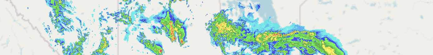
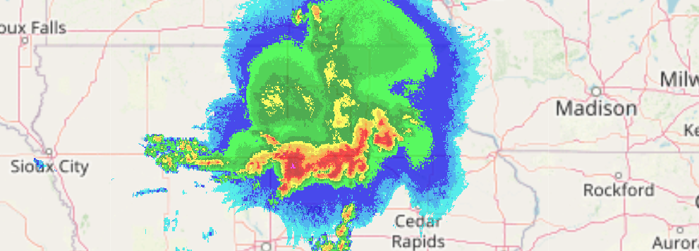
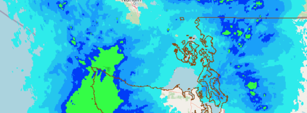
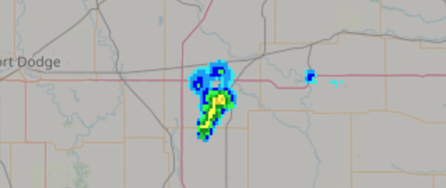
reflectivity_plot

Above is your visualization! You can use the menu bar at the upper right side of the plot to pan around the plot, zoom in to a region of interest, and reset your selections to the default map. If you mouse over the values on the screen, you will see the latitude, longitude, and value associated with the selected product.

🏆 Bonus Challenges¶

Congratulations on the completion of this notebook! You have successfully selected a region and product, queried the AWS S3 bucket, and visualized MRMS data in near real-time.

If you’d like to continue this analysis, I’ve provided a couple of bonus challenges. Click on the drop-down menu to view the bonus challenge according to your desired level of difficulty.

Browse the AWS S3 bucket and the NSSL Variable Table and find an MRMS product that was not covered in this notebook. Alter the provided code to read in and plot your new variable!

Step-by-step:

Delete the widget-generating cell in the “Data selection” section.
Hard-code the “region” and “product” variables with the exact strings that correspond to your data product on AWS. For example:
```
region = "CONUS" 
product = "MergedReflectivityQCComposite_00.50"
```
Run the rest of the notebook cells to produce your plot.

Troubleshooting:

If your data request step returns an error, go to the AWS S3 bucket and manually click through your selection. Is the data there? Did you copy the product and region variable names exactly as they are in S3?
Some datasets have different values to indicate that the data is missing, range folded, or not covered. You can find this information in the NSSL talbe. If your data has unique values, you may need to mask it in the plotting step to make sure the colorbar works for your dataset.

Turn this notebook into a Python script, then use cron to create an updated plot from MRMS data every hour. Incorporate this plot into a web page, send it to your friend, or try it just for fun!

Step-by-step:

Delete the widget-generating cell in the “Data selection” section.
Hard-code the “region” and “product” variables with the exact strings that correspond to your data product on AWS. For example:
```
region = "CONUS" 
product = "MergedReflectivityQCComposite_00.50"
```
Delete the hvplot-generating cell in the “Visualization” section.
Use the static plotting code located in the appendix for your visualization, or write your own static plotting code. Change the filepath in plt.savefig() to an absolute path to ensure that your plot will be saved in a known, designated location.
(optional) Delete all markdown cells in the notebook to make your code sections more clearly delineated.
Organize the import statements, removing any unnecessary imports (such as those associated with widgets and the hvplot) and duplicates.
Restart the notebook, clear all outputs, and run the cells again to confirm that the output is a single, static plot with the most recent time stamp. If everything executed as expected, you may continue. If you ran into any errors, now is the time to troubleshoot!
Create a .py file, and copy your Jupyter Notebook cells chronologically into this file.

Now, the exact way you go about creating a cron-ready file is up to you. You can apply your current cron workflow (if one exists), paste your current .py script into your favorite GenAI programming tool for help, or find online resources that list cron best practices.

Here is what I did:

Organized my Python code into two functions: retrieve_data() and plot_data(). I execute these functions under the block if __name__ == "__main__":, using input from retrieve_data() as an argument to plot_data().
Added “try” and “except” blocks and logging in case of failure.
Saved the Python file as mrms_cron.py, tested my code manually in its virtual environment (~/myenv/bin/python ~/scripts/mrms_cron.py ; make sure to update the file paths to reflect your own environment), then ensured that the plotting output appeared in its designated location and looked correct.
Made my script executable by typing chmod +x ~/scripts/mrms_cron.py (again, make sure you enter your own file path) into the command line.
Edited my crontab (in the command line: crontab -e) to run my script 10 minutes after every hour (10 * * * * /home/user/myenv/bin/python /home/user/scripts/mrms_cron.py >> /home/user/mrms_output/mrms.log 2>&1).
The next time HH:10 rolled around, I waited a couple minutes for the plot to generate, then checked the file path that I designated to contain my images. There it was!

📚 Resources and references¶

AWS Data Access:

AWS S3 bucket for MRMS data

MRMS Information:

🛠️ Appendix¶

If you’d prefer to plot these data as a static plot, below is some sample code to kickstart your plotting journey.

"""
import matplotlib.pyplot as plt
import cartopy.crs as ccrs
import cartopy.feature as cfeature
import pandas as pd
from metpy.plots import ctables

# Mask data for neater visualization
data = data.where(data > 0, np.nan)

# Extract data
lons = data.longitude
lats = data.latitude
values = data.values
date = pd.to_datetime(data.time.values)

# Domain bounds
minLon, maxLon = lons.min(), lons.max()
minLat, maxLat = lats.min(), lats.max()

# Setup figure and axis
fig, ax = plt.subplots(figsize=(12, 6),
                       subplot_kw={"projection": ccrs.Mercator()})

ax.set_extent([minLon, maxLon, minLat, maxLat], crs=ccrs.PlateCarree())

# Set colors
ref_norm, ref_cmap = ctables.registry.get_with_steps("NWSReflectivity", 5, 5)
units = "Reflectivity (dBZ)"
title = "MRMS Merged Reflectivity"

# Add features
ax.add_feature(cfeature.STATES, linewidth=0.5)
ax.add_feature(cfeature.BORDERS, linewidth=0.7)

# Plot data
radarplot = ax.pcolormesh(
    lons, lats, values,
    transform=ccrs.PlateCarree(),
    cmap=ref_cmap, norm=ref_norm,
    shading="auto"
)

# Colorbar
cbar = fig.colorbar(radarplot, ax=ax, orientation="vertical", pad=0.02)
cbar.set_label(units)

# Titles
ax.set_title(title, loc="left", fontweight="bold")
ax.set_title(date.strftime("%d %B %Y at %H:%M UTC"), loc="right")

png_name = f"mrms_{region}_{product}_{date.strftime('%Y%m%d_%H%M%S')}.png"
plt.savefig(png_name, dpi=150, bbox_inches="tight")
plt.close(fig)
"""

'\nimport matplotlib.pyplot as plt\nimport cartopy.crs as ccrs\nimport cartopy.feature as cfeature\nimport pandas as pd\nfrom metpy.plots import ctables\n\n# Mask data for neater visualization\ndata = data.where(data > 0, np.nan)\n\n# Extract data\nlons = data.longitude\nlats = data.latitude\nvalues = data.values\ndate = pd.to_datetime(data.time.values)\n\n# Domain bounds\nminLon, maxLon = lons.min(), lons.max()\nminLat, maxLat = lats.min(), lats.max()\n\n# Setup figure and axis\nfig, ax = plt.subplots(figsize=(12, 6),\n                       subplot_kw={"projection": ccrs.Mercator()})\n\nax.set_extent([minLon, maxLon, minLat, maxLat], crs=ccrs.PlateCarree())\n\n# Set colors\nref_norm, ref_cmap = ctables.registry.get_with_steps("NWSReflectivity", 5, 5)\nunits = "Reflectivity (dBZ)"\ntitle = "MRMS Merged Reflectivity"\n\n# Add features\nax.add_feature(cfeature.STATES, linewidth=0.5)\nax.add_feature(cfeature.BORDERS, linewidth=0.7)\n\n# Plot data\nradarplot = ax.pcolormesh(\n    lons, lats, values,\n    transform=ccrs.PlateCarree(),\n    cmap=ref_cmap, norm=ref_norm,\n    shading="auto"\n)\n\n# Colorbar\ncbar = fig.colorbar(radarplot, ax=ax, orientation="vertical", pad=0.02)\ncbar.set_label(units)\n\n# Titles\nax.set_title(title, loc="left", fontweight="bold")\nax.set_title(date.strftime("%d %B %Y at %H:%M UTC"), loc="right")\n\npng_name = f"mrms_{region}_{product}_{date.strftime(\'%Y%m%d_%H%M%S\')}.png"\nplt.savefig(png_name, dpi=150, bbox_inches="tight")\nplt.close(fig)\n'

Footnotes¶

Merged Reflectivity Composite

Description: The maximum reflectivity in a vertical column, from the merged product.
Spatial Resolution: 0.01º Latitude (~1.11 km) x 0.01º Longitude (~1.01 km at 25ºN and 0.73 km at 49ºN)
Temporal Resolution: 2 minutes
AWS Variable: “MergedReflectivityQCComposite_00.50”
↩
12-hour Multisensor Quantitative Precipitation Estimate (Pass 2)
Description: 12h rainfall accumulation estimate, using data from rain gauges and NWP QPF (HRRR/RAP blend for CONUS). This is the Pass 2 dataset, which has a higher latency but includes more rain gauge data than Pass 1 (Pass 1 has 20-minute latency and includes 10% of gauges, while Pass 2 has 60-minute latency and includes 60% of gauges).
Spatial Resolution: 1km x 1km
Temporal Resolution: 60 minutes
AWS Variable: “MultiSensor_QPE_12H_Pass2_00.00”
↩
Probability of Severe Hail
Description: The probability of 0.75-inch diameter hail.
Spatial Resolution: 0.01º Latitude (~1.11 km) x 0.01º Longitude (~1.01 km at 25ºN and 0.73 km at 49ºN)
Temporal Resolution: 2 minutes
AWS Variable: “POSH_00.50”
↩

MRMS Cookbook

NOAA Multi-Radar / Multi-Sensor System (MRMS) at the BNF Field Site(s)