The NA-CORDEX data archive contains output from regional climate models (RCMs) run over a domain covering most of North America using boundary conditions from global climate model (GCM) simulations in the CMIP5 archive. It differs from many climate datasets by combining runs from many independently derived simulations. The usage of Zarr, Xarray, and Intake-ESM help simplify the problem of examining these disparate runs.
See the README file for more pointers and information on the NA-CORDEX data archive.
Overview
This cookbook provides useful methods for summarizing data values in large climate datasets. It clearly shows where data have extreme values and where data are missing; this can be useful for validating that the data were gathered and stored correctly. While this cookbook is specifically designed to examine any portion of the NA-CORDEX dataset using an intake catalog, the code can be adapted straightforwardly to other datasets that can be loaded via xarray.
Topics covered in this notebook include:
Different Ways to Create and Connect to Dask Distributed Cluster
How to Find and Obtain Data Using an Intake-ESM Catalog
How to Create Various Statistical Summary Plots with matplotlib
Prerequisites
To more fully understand how the code in this notebook works, users are encouraged to explore the following introductory articles.
| Concepts | Importance | Notes |
|---|---|---|
| Intro to Xarray | Helpful | |
| Dask Arrays with Xarray | Helpful | |
| Understanding of Zarr Metadata | Helpful | Familiarity with metadata structure |
| Understanding of Matplotlib | Helpful | Familiarity with plot elements in matplotlib |
Time to learn: 45 minutes
Note: This notebook contains optional choices for running on NCAR supercomputers. These can be ignored for users running outside of the NCAR domain.
Imports
The main python packages used are xarray, intake-esm, dask, and matplotlib.
Because some of the CORDEX data have been interpolated from a Lambert Conformal grid onto a rectangular grid for ease of use, there can be many missing values on the edges of the interpolated grid. For this reason, we also turn off warnings complaining about missing values in the data.
import xarray as xr
import numpy as np
import intake
import ast
import matplotlib.pyplot as plt

# Ignore dask-numpy warnings about finding missing values in the data
%env PYTHONWARNINGS=ignore
env: PYTHONWARNINGS=ignore
Select User Options
Users may choose between:
Cloud storage provider (Amazon AWS or NCAR),
Whether to truncate the data if running on a resource-limited computer,
Whether to obtain a Dask cluster from a PBS Scheduler or via the Dask Gateway package.
Note: Using the NCAR cloud storage system requires a login account on an NCAR HPC computer.
Choose Cloud Storage (Amazon AWS or NCAR Cloud)
# If True,  use NCAR Cloud Storage.   Requires an NCAR user account.
# If False, use AWS  Cloud Storage.

USE_NCAR_CLOUD = False
Choose whether to truncate data for resource-limited computers
When running this notebook where compute resources are limited, or data transfer rates are slow, set TRUNCATE_DATA to True. This will limit time ranges to 3 years from the start of a chosen NA-CORDEX scenario.
TRUNCATE_DATA = TrueChoose whether to use a PBS Scheduler
If running on a HPC computer with a PBS Scheduler, set to True. Otherwise, set to False.
USE_PBS_SCHEDULER = FalseChoose whether to use Dask Gateway
If running on Jupyter server with Dask Gateway configured, set to True. Otherwise, set to False.
USE_DASK_GATEWAY = FalseCreate and Connect to Dask Distributed Cluster
def get_gateway_cluster():
    """ Create cluster through dask_gateway
    """
    from dask_gateway import Gateway

    gateway = Gateway()
    cluster = gateway.new_cluster()
    cluster.adapt(minimum=2, maximum=20)
    return cluster
def get_pbs_cluster():
""" Create cluster through dask_jobqueue
"""
from dask_jobqueue import PBSCluster
if TRUNCATE_DATA:
num_jobs = 4
walltime = '0:10:00'
memory = '2GB'
else:
num_jobs = 20
walltime = '0:20:00'
memory = '10GB'
cluster = PBSCluster(cores=1, processes=1, walltime=walltime, memory=memory, queue='casper',
resource_spec=f"select=1:ncpus=1:mem={memory}",)
cluster.scale(jobs=num_jobs)
return clusterdef get_local_cluster():
""" Create cluster using the Jupyter server's resources
"""
from distributed import LocalCluster
cluster = LocalCluster()
if TRUNCATE_DATA:
cluster.scale(4)
else:
cluster.scale(20)
return cluster# Obtain dask cluster in one of three ways
if USE_PBS_SCHEDULER:
cluster = get_pbs_cluster()
elif USE_DASK_GATEWAY:
cluster = get_gateway_cluster()
else:
cluster = get_local_cluster()
# Connect to cluster
from distributed import Client
client = Client(cluster)
# Display cluster dashboard URL
cluster☝️ Link to Dask dashboard will appear above.
Find and Obtain Data Using an Intake Catalog
Define the Intake Catalog URL and Storage Access Options
if USE_NCAR_CLOUD:
    catalog_url = "https://stratus.ucar.edu/ncar-na-cordex/catalogs/aws-na-cordex.json"
    storage_options={"anon": True, 'client_kwargs':{"endpoint_url":"https://stratus.ucar.edu/"}}

else:
    catalog_url = "https://ncar-na-cordex.s3-us-west-2.amazonaws.com/catalogs/aws-na-cordex.json"
    storage_options={"anon": True}
Open catalog and produce a content summary
# Have the catalog interpret the "na-cordex-models" column as a list of values, as opposed to single values.
col = intake.open_esm_datastore(catalog_url, read_csv_kwargs={"converters": {"na-cordex-models": ast.literal_eval}},)
col
/tmp/ipykernel_4503/2356137384.py:2: DeprecationWarning: read_csv_kwargs is deprecated and will be removed in a future version. Please use read_kwargs instead.
col = intake.open_esm_datastore(catalog_url, read_csv_kwargs={"converters": {"na-cordex-models": ast.literal_eval}},)
# Show the first few lines of the catalog
col.df.head(10)# Produce a catalog content summary.
uniques = col.unique()
columns = ["variable", "scenario", "grid", "na-cordex-models", "bias_correction"]
for column in columns:
print(f'{column}: {uniques[column]}\n')variable: ['hurs', 'huss', 'pr', 'prec', 'ps', 'rsds', 'sfcWind', 'tas', 'tasmax', 'tasmin', 'temp', 'tmax', 'tmin', 'uas', 'vas']
scenario: ['eval', 'hist-rcp45', 'hist-rcp85', 'hist', 'rcp45', 'rcp85']
grid: ['NAM-22i', 'NAM-44i']
na-cordex-models: ['ERA-Int.CRCM5-UQAM', 'ERA-Int.CRCM5-OUR', 'ERA-Int.RegCM4', 'ERA-Int.CanRCM4', 'ERA-Int.WRF', 'ERA-Int.HIRHAM5', 'ERA-Int.RCA4', 'CanESM2.CanRCM4', 'GFDL-ESM2M.CRCM5-OUR', 'CanESM2.CRCM5-OUR', 'MPI-ESM-LR.CRCM5-UQAM', 'CanESM2.CRCM5-UQAM', 'EC-EARTH.HIRHAM5', 'EC-EARTH.RCA4', 'CanESM2.RCA4', 'MPI-ESM-MR.CRCM5-UQAM', 'GEMatm-Can.CRCM5-UQAM', 'GEMatm-MPI.CRCM5-UQAM', 'HadGEM2-ES.RegCM4', 'GFDL-ESM2M.RegCM4', 'MPI-ESM-LR.RegCM4', 'HadGEM2-ES.WRF', 'GFDL-ESM2M.WRF', 'MPI-ESM-LR.WRF', 'CNRM-CM5.CRCM5-OUR', 'MPI-ESM-LR.CRCM5-OUR']
bias_correction: ['raw', 'mbcn-Daymet', 'mbcn-gridMET']
Load data into xarray using the catalog
Choose any combination of variable, grid, scenario, and bias correction listed in the catalog.
Below we choose the variable ‘tmax’ (Maximum Daily Surface Temperature) as a default for its ease of interpretation. For this example, we also choose a lower-resolution grid and the scenario with the shortest time range (15 years) to reduce the default data processing requirements.
data_var = 'tmax'

col_subset = col.search(
    variable=data_var,
    grid="NAM-44i",
    scenario="eval",
    bias_correction="raw",
)

col_subset# Verify our query matches at least one entry in the catalog.
col_subset.df# Load catalog entries for subset into a dictionary of xarray datasets, and open the first one.
dsets = col_subset.to_dataset_dict(
xarray_open_kwargs={"consolidated": True}, storage_options=storage_options
)
print(f"\nDataset dictionary keys:\n {dsets.keys()}")
# Load the first dataset and display a summary.
dataset_key = list(dsets.keys())[0]
store_name = dataset_key + ".zarr"
ds = dsets[dataset_key]
ds
# Note that the xarray dataset summary includes a 'member_id' coordinate, which is a renaming of the
# 'na-cordex-models' column in the catalog.
--> The keys in the returned dictionary of datasets are constructed as follows:
	'variable.frequency.scenario.grid.bias_correction'
Dataset dictionary keys:
 dict_keys(['tmax.day.eval.NAM-44i.raw'])
Functions for Subsetting and Plotting
Helper Function to Create a Single Map Plot
def plotMap(ax, map_slice, date_object=None, member_id=None):
    """Create a map plot on the given axes, with min/max as text"""

    ax.imshow(map_slice, origin='lower')

    minval = map_slice.min(dim = ['lat', 'lon'])
    maxval = map_slice.max(dim = ['lat', 'lon'])

    # Format values to have at least 4 digits of precision.
    ax.text(0.01, 0.03, "Min: %3g" % minval, transform=ax.transAxes, fontsize=12)
    ax.text(0.99, 0.03, "Max: %3g" % maxval, transform=ax.transAxes, fontsize=12, horizontalalignment='right')
    ax.set_xticks([])
    ax.set_yticks([])

    if date_object:
        ax.set_title(date_object.values.astype(str)[:10], fontsize=12)

    if member_id:
        ax.set_ylabel(member_id, fontsize=12)

    return ax
Helper Function for Finding Dates with Available Data
def getValidDateIndexes(member_slice):
    """Search for the first and last dates with finite values."""
    min_values = member_slice.min(dim = ['lat', 'lon'])
    is_finite = np.isfinite(min_values)
    finite_indexes = np.where(is_finite)

    start_index = finite_indexes[0][0]
    end_index = finite_indexes[0][-1]
    return start_index, end_index
Helper Function for Truncating Data Slices
def truncateData(data_slice, num_years):
    """Remove all but the first num_years of valid data from the data slice."""
    start_index, _ = getValidDateIndexes(data_slice)
    start_date = data_slice.time[start_index]
    start_year = start_date.dt.year.values
    year_range = start_year + np.arange(num_years)

    data_slice = data_slice.isel(time=ds.time.dt.year.isin(year_range))
    return data_slice
Function Producing Maps of First, Middle, and Final Timesteps
def plot_first_mid_last(ds, data_var, store_name):
    """Plot the first, middle, and final time steps for several climate runs."""
    num_members_to_plot = 4
    member_names = ds.coords['member_id'].values[0:num_members_to_plot]

    figWidth = 18
    figHeight = 12
    numPlotColumns = 3
    fig, axs = plt.subplots(num_members_to_plot, numPlotColumns, figsize=(figWidth, figHeight), constrained_layout=True)

    for index in np.arange(num_members_to_plot):
        mem_id = member_names[index]
        data_slice = ds[data_var].sel(member_id=mem_id)

        start_index, end_index = getValidDateIndexes(data_slice)
        midDateIndex = np.floor(len(ds.time) / 2).astype(int)

        startDate = ds.time[start_index]
        first_step = data_slice.sel(time=startDate)
        ax = axs[index, 0]
        plotMap(ax, first_step, startDate, mem_id)

        midDate = ds.time[midDateIndex]
        mid_step = data_slice.sel(time=midDate)
        ax = axs[index, 1]
        plotMap(ax, mid_step, midDate)

        endDate = ds.time[end_index]
        last_step = data_slice.sel(time=endDate)
        ax = axs[index, 2]
        plotMap(ax, last_step, endDate)

        plt.suptitle(f'First, Middle, and Last Timesteps for Selected Runs in "{store_name}"', fontsize=20)

    return fig
Function Producing Statistical Map Plots
def plot_stat_maps(ds, data_var, store_name, truncate_data):
    """Plot the mean, min, max, and standard deviation values for several climate runs, aggregated over time."""

    num_members_to_plot = 4
    member_names = ds.coords['member_id'].values[0:num_members_to_plot]

    figWidth = 25
    figHeight = 12
    numPlotColumns = 4

    fig, axs = plt.subplots(num_members_to_plot, numPlotColumns, figsize=(figWidth, figHeight), constrained_layout=True)

    for index in np.arange(num_members_to_plot):
        mem_id = member_names[index]
        data_slice = ds[data_var].sel(member_id=mem_id)

        if truncate_data:
            # Limit time range to one year.
            data_slice = truncateData(data_slice, 1)

        # Save slice in memory to prevent repeated disk loads
        data_slice = data_slice.persist()

        data_agg = data_slice.min(dim='time')
        plotMap(axs[index, 0], data_agg, member_id=mem_id)

        data_agg = data_slice.max(dim='time')
        plotMap(axs[index, 1], data_agg)

        data_agg = data_slice.mean(dim='time')
        plotMap(axs[index, 2], data_agg)

        data_agg = data_slice.std(dim='time')
        plotMap(axs[index, 3], data_agg)

    axs[0, 0].set_title(f'min({data_var})', fontsize=15)
    axs[0, 1].set_title(f'max({data_var})', fontsize=15)
    axs[0, 2].set_title(f'mean({data_var})', fontsize=15)
    axs[0, 3].set_title(f'std({data_var})', fontsize=15)

    plt.suptitle(f'Spatial Statistics for Selected Runs in "{store_name}"', fontsize=20)

    return fig
Function Producing Time Series Plots
Also show which dates have no available data values, as a rug plot.
def plot_timeseries(ds, data_var, store_name, truncate_data):
    """Plot the mean, min, max, and standard deviation values for several climate runs,
       aggregated over lat/lon dimensions."""

    num_members_to_plot = 4
    member_names = ds.coords['member_id'].values[0:num_members_to_plot]

    figWidth = 25
    figHeight = 20
    linewidth = 0.5

    numPlotColumns = 1
    fig, axs = plt.subplots(num_members_to_plot, numPlotColumns, figsize=(figWidth, figHeight))

    for index in np.arange(num_members_to_plot):
        mem_id = member_names[index]
        data_slice = ds[data_var].sel(member_id=mem_id)

        if truncate_data:
            # Limit time range to one year.
            data_slice = truncateData(data_slice, 1)

        # Save slice in memory to prevent repeated disk loads
        data_slice = data_slice.persist()

        unit_string = ds[data_var].attrs['units']

        min_vals = data_slice.min(dim = ['lat', 'lon'])
        max_vals = data_slice.max(dim = ['lat', 'lon'])
        mean_vals = data_slice.mean(dim = ['lat', 'lon'])
        std_vals = data_slice.std(dim = ['lat', 'lon'])

        missing_indexes = np.isnan(min_vals).compute()
        missing_times = data_slice.time[missing_indexes]


        axs[index].plot(data_slice.time, max_vals, linewidth=linewidth, label='max', color='red')
        axs[index].plot(data_slice.time, mean_vals, linewidth=linewidth, label='mean', color='black')
        axs[index].fill_between(data_slice.time, (mean_vals - std_vals), (mean_vals + std_vals),
                                         color='grey', linewidth=0, label='std', alpha=0.5)
        axs[index].plot(data_slice.time, min_vals, linewidth=linewidth, label='min', color='blue')

        # Produce a rug plot along the bottom of the figure for missing data.
        ymin, ymax = axs[index].get_ylim()
        rug_y = ymin + 0.01*(ymax-ymin)
        axs[index].plot(missing_times, [rug_y]*len(missing_times), '|', color='m', label='missing')
        axs[index].set_title(mem_id, fontsize=20)
        axs[index].legend(loc='upper right')
        axs[index].set_ylabel(unit_string)

    plt.tight_layout(pad=10.2, w_pad=3.5, h_pad=3.5)
    plt.suptitle(f'Temporal Statistics for Selected Runs in "{store_name}"', fontsize=20)

    return fig
Produce Diagnostic Plots
Plot First, Middle, and Final Timesteps for Several Output Runs (less compute intensive)
%%time

# Plot using the Zarr Store obtained from an earlier step in the notebook.
figure = plot_first_mid_last(ds, data_var, store_name)

plt.show()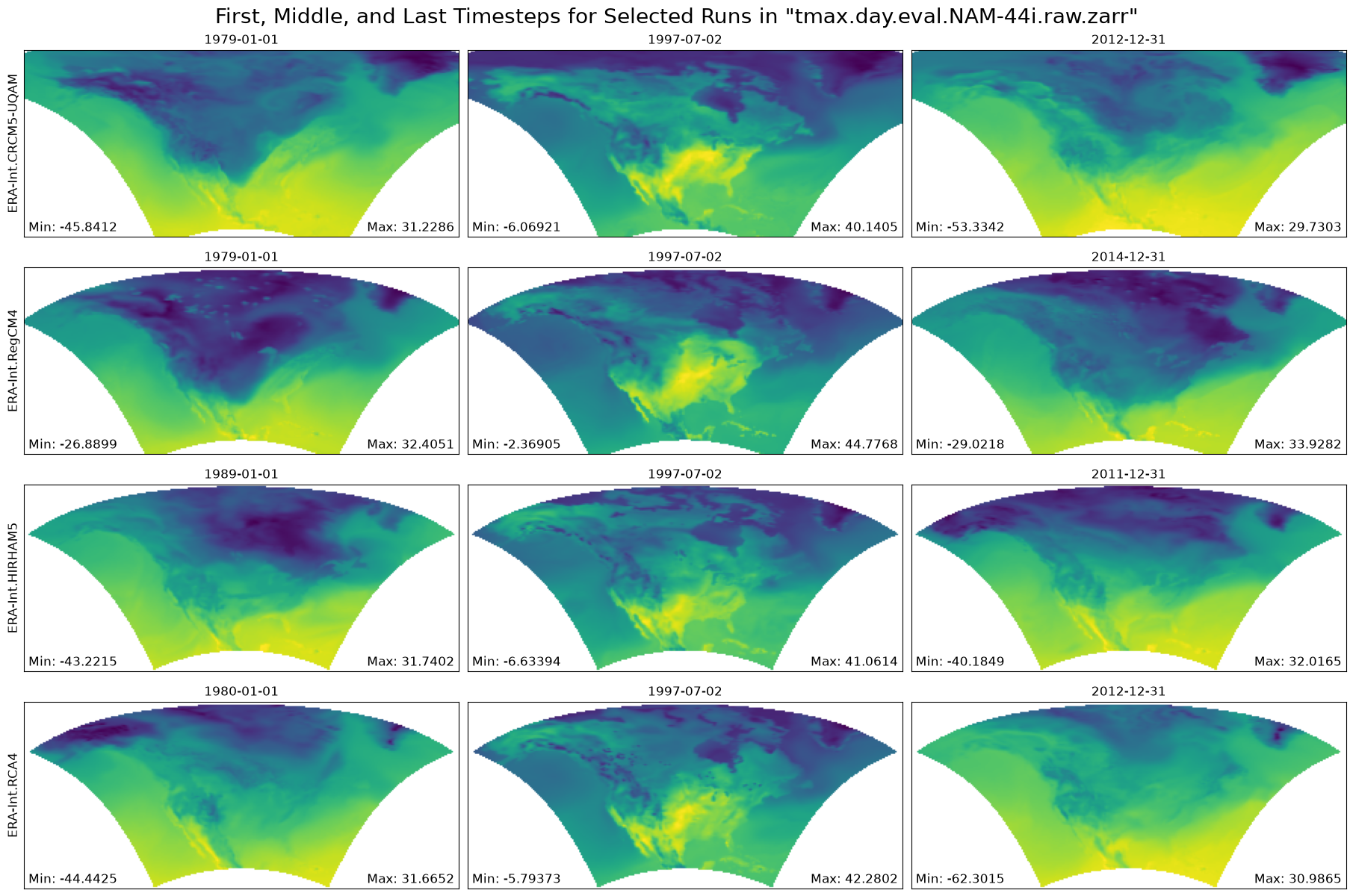
CPU times: user 7.36 s, sys: 1.88 s, total: 9.25 s
Wall time: 3min
Optional: Save figure to a PNG file
Change the value of SAVE_PLOT to True to produce a PNG file of the plot. The file will be saved in the same folder as this notebook.
Then use Jupyter’s file browser to locate the file and right-click the file to download it.
SAVE_PLOT = False
if SAVE_PLOT:
    plotfile = f'./{dataset_key}_FML.png'
    figure.savefig(plotfile, dpi=100)
Create Statistical Map Plots for Several Output Runs (more compute intensive)
%%time

# Plot using the Zarr Store obtained from an earlier step in the notebook.
figure = plot_stat_maps(ds, data_var, store_name, TRUNCATE_DATA)

plt.show()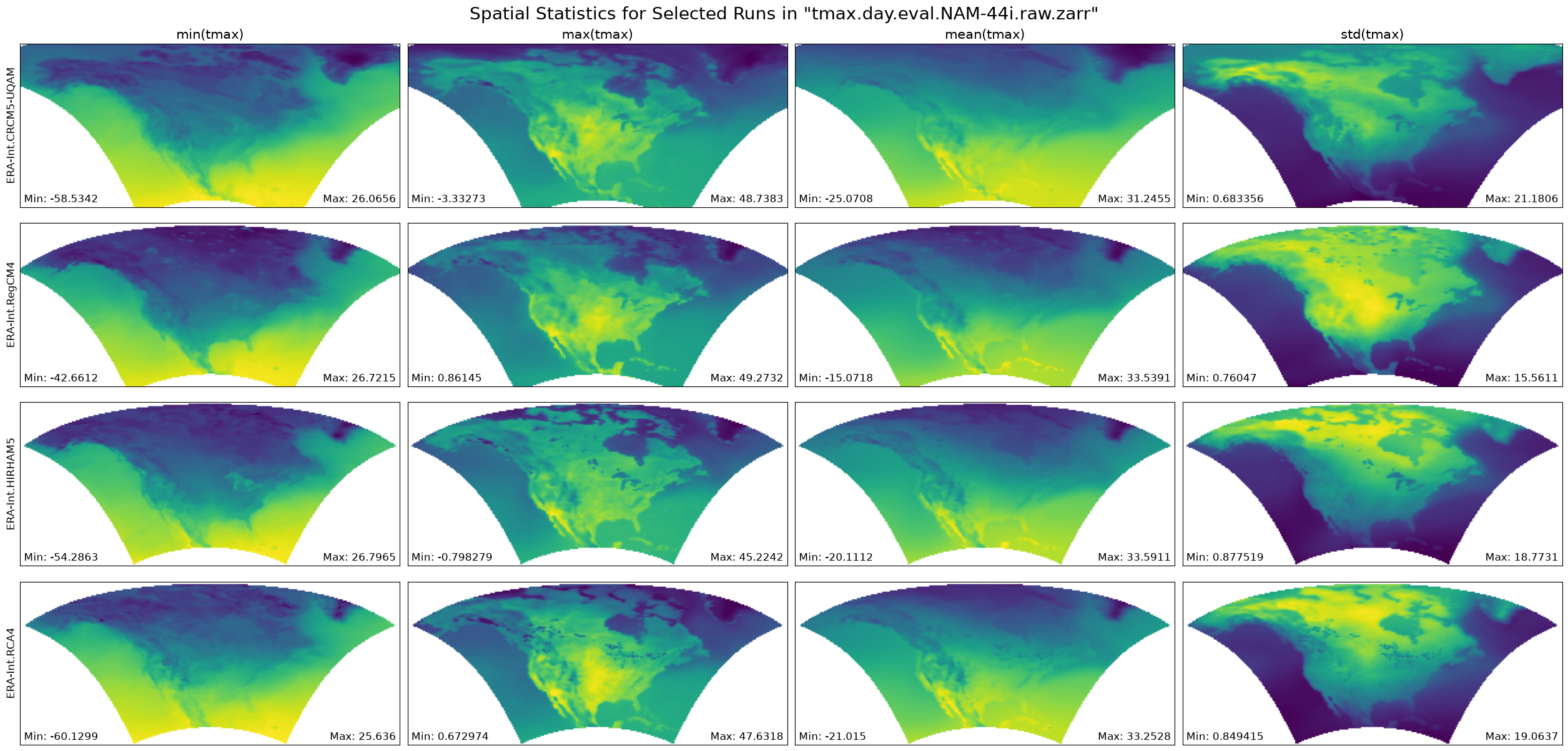
CPU times: user 5.94 s, sys: 1.16 s, total: 7.1 s
Wall time: 1min 56s
Optional: Save figure to a PNG file
Change the value of SAVE_PLOT to True to produce a PNG file of the plot. The file will be saved in the same folder as this notebook.
Then use Jupyter’s file browser to locate the file and right-click the file to download it.
SAVE_PLOT = False
if SAVE_PLOT:
    plotfile = f'./{dataset_key}_MAPS.png'
    figure.savefig(plotfile, dpi=100)
Plot Time Series for Several Output Runs (more compute intensive)
%%time

# Plot using the Zarr Store obtained from an earlier step in the notebook.
figure = plot_timeseries(ds, data_var, store_name, TRUNCATE_DATA)

plt.show()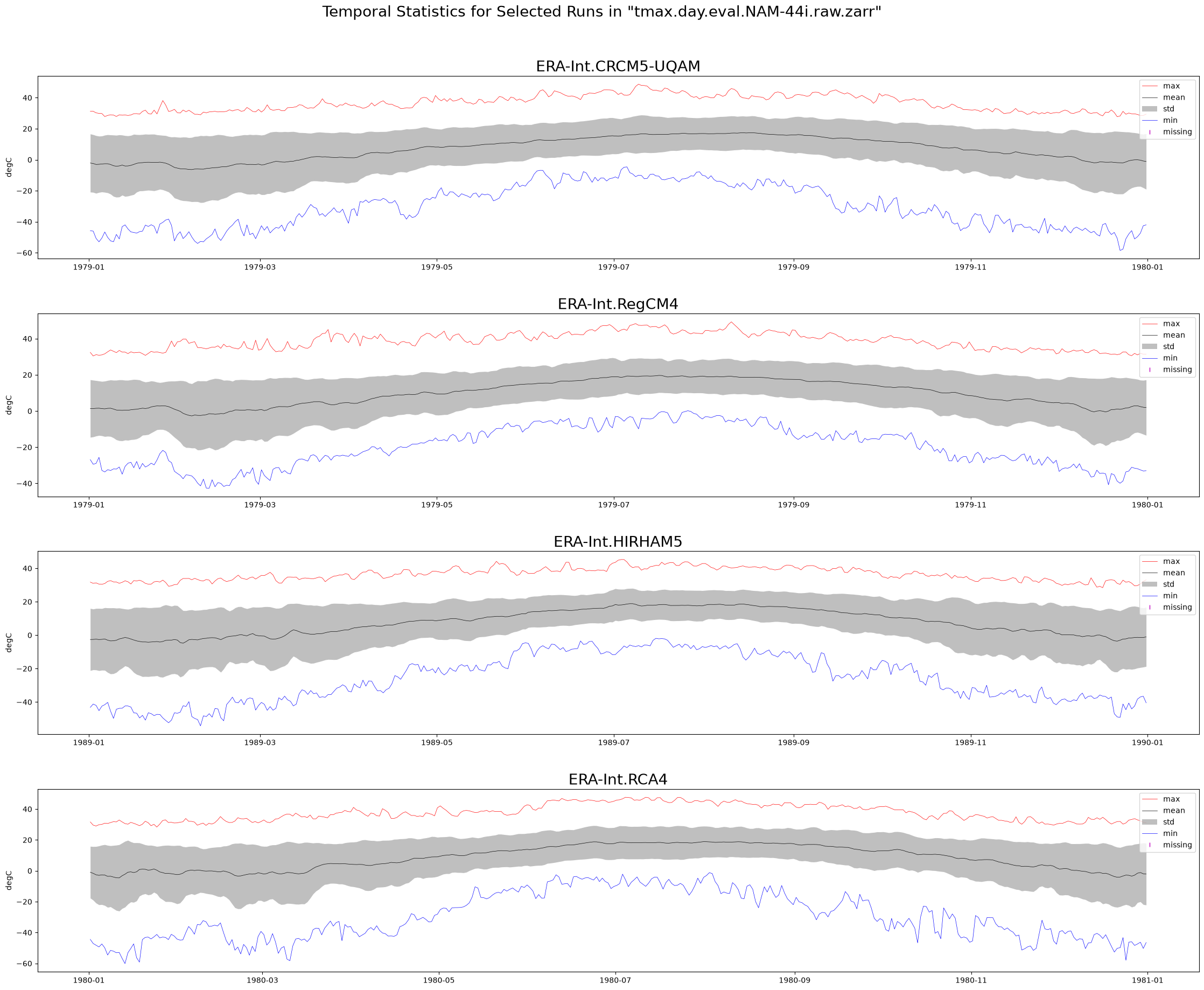
CPU times: user 5.22 s, sys: 1.04 s, total: 6.26 s
Wall time: 1min 38s
Optional: Save figure to a PNG file
Change the value of SAVE_PLOT to True to produce a PNG file of the plot. The file will be saved in the same folder as this notebook.
Then use Jupyter’s file browser to locate the file and right-click the file to download it.
SAVE_PLOT = False
if SAVE_PLOT:
    plotfile = f'./{dataset_key}_TS.png'
    figure.savefig(plotfile, dpi=100)
Release the workers.
!dateSun Oct 11 03:33:32 UTC 2026
cluster.close()Unclosed client session
client_session: <aiohttp.client.ClientSession object at 0x7fbda8ea0cd0>
Unclosed connector
connections: ['deque([(<aiohttp.client_proto.ResponseHandler object at 0x7fbda8129a50>, 565.785889727), (<aiohttp.client_proto.ResponseHandler object at 0x7fbda3da0c50>, 566.788586753)])']
connector: <aiobotocore.httpsession._ProxySSLTCPConnector object at 0x7fbda8e52f50>
Unclosed client session
client_session: <aiohttp.client.ClientSession object at 0x7fb2381d6ad0>
Unclosed connector
connections: ['deque([(<aiohttp.client_proto.ResponseHandler object at 0x7fb2333dfa50>, 566.150231974), (<aiohttp.client_proto.ResponseHandler object at 0x7fb23328d5d0>, 567.037698655)])']
connector: <aiobotocore.httpsession._ProxySSLTCPConnector object at 0x7fb2381e7010>
Unclosed client session
client_session: <aiohttp.client.ClientSession object at 0x7f5cc87f6f90>
Unclosed connector
connections: ['deque([(<aiohttp.client_proto.ResponseHandler object at 0x7f5caa2e3cd0>, 565.784205274), (<aiohttp.client_proto.ResponseHandler object at 0x7f5caa2f20d0>, 566.997285396)])']
connector: <aiobotocore.httpsession._ProxySSLTCPConnector object at 0x7f5cc83c3610>
Show which python package versions were used
%load_ext watermark
%watermark -iv
distributed: 2026.8.0
intake : 2.0.9
matplotlib : 3.11.2
numpy : 2.4.6
xarray : 2026.9.0