Specific Differential Phase (\(K_{DP}\)) retrieval methods comparison

Overview

Within this notebook, we will cover:

How to access Colombian national weather radar network data from AWS
How to read and create a multipanel plot
How to retrieve and compare three different methods

Prerequisites

Concepts	Importance	Notes
Matplotlib Basics	Required	Basic plotting
Introduction to Cartopy	Helpful	Adding projections to your plot
Py-ART Basics	Required	IO/Visualization
Py-ART Corrections	Required	Radar Corrections
Py-ART Example-workflows	Required	Dual-polarization variables

Imports

import xradar as xd
import pyart
import xarray as xr
import numpy as np
import fsspec
import matplotlib.pyplot as plt
import cartopy.crs as ccrs
from open_radar_data import DATASETS
import matplotlib.ticker as mticker
import warnings

warnings.filterwarnings("ignore")

## You are using the Python ARM Radar Toolkit (Py-ART), an open source
## library for working with weather radar data. Py-ART is partly
## supported by the U.S. Department of Energy as part of the Atmospheric
## Radiation Measurement (ARM) Climate Research Facility, an Office of
## Science user facility.
##
## If you use this software to prepare a publication, please cite:
##
##     JJ Helmus and SM Collis, JORS 2016, doi: 10.5334/jors.119

How to access Colombian national weather radar network data from AWS

Let’s start first with Level 2 radar data, which is ground-based radar data collected by the Instituto de Hidrología, Meteorología y Estudios Ambientales (IDEAM).

Level 2 Data

Level 2 data includes all of the fields in a single file - for example, a file may include:

Reflectivity
Velocity
Differential reflectivity

Search for data during a Mesoscale Convective System - MCS event (August 9, 2022)

We will access data from the radaresideam bucket, with the data organized as:

s3://s3-radaresideam/l2_data/year/month/date/radar_name/{radar_name[:3].upper()}{year}{month}{date}{hour}{minute}{second}.RAW*

We can use fsspec, a tool to work with filesystems in Python, to search through the bucket to find our files!

We start first by setting up our AWS S3 filesystem

fs = fsspec.filesystem("s3", anon=True)

Now, we can list files from August 9, 2022, from Carimagua radar (CAR), around 1900 UTC.

files = sorted(fs.glob("s3-radaresideam/l2_data/2022/08/09/Carimagua/CAR22080919*"))
files[:4]

['s3-radaresideam/l2_data/2022/08/09/Carimagua/CAR220809190003.RAWDSVV',
 's3-radaresideam/l2_data/2022/08/09/Carimagua/CAR220809190315.RAWDSW0',
 's3-radaresideam/l2_data/2022/08/09/Carimagua/CAR220809190401.RAWDSW3',
 's3-radaresideam/l2_data/2022/08/09/Carimagua/CAR220809190505.RAWDSW8']

Read the data into Py-ART

When reading into Py-ART, we can use the pyart.io.read_sigmet or pyart.io.read module to read in our data.

radar = pyart.io.read_sigmet(f's3://{files[7]}')

List the available fields

sorted(list(radar.fields))

['cross_correlation_ratio',
 'differential_phase',
 'differential_reflectivity',
 'normalized_coherent_power',
 'radar_echo_classification',
 'reflectivity',
 'specific_differential_phase',
 'spectrum_width',
 'total_power',
 'velocity']

Plot dual-pol variables

Let’s plot the radar reflectivity (\(Z\)), differential reflectivity (\(Z_{DR}\)), specific differential phase (\(K_{DP}\)), and cross correlation ratio (\(\rho_{HV}\)) using a four panel plot.

fig = plt.figure(figsize=(12,10))
display = pyart.graph.RadarMapDisplay(radar)
# Extract the latitude and longitude of the radar and use it for the center of the map
lat_center = round(radar.latitude['data'][0], 0)
lon_center = round(radar.longitude['data'][0], 0)


# Determine the ticks
lat_ticks = np.arange(lat_center-3, lat_center+3, 1.5)
lon_ticks = np.arange(lon_center-3, lon_center+3, 1.5)

# Set the projection - in this case, we use a general PlateCarree projection
projection = ccrs.PlateCarree()
ax1 = plt.subplot(221, projection=projection)
display.plot_ppi_map("reflectivity", 0, 
                     resolution='10m', 
                     ax=ax1, 
                     lat_lines=lat_ticks, 
                     lon_lines=lon_ticks)

ax2 = plt.subplot(222, projection=projection)
display.plot_ppi_map("differential_reflectivity", 0, 
                     resolution='10m', 
                     ax=ax2, 
                     lat_lines=lat_ticks, 
                     lon_lines=lon_ticks)

ax3 = plt.subplot(223, projection=projection)
display.plot_ppi_map("differential_phase", 0, 
                     vmin=0, vmax=180,  
                     ax=ax3, resolution='10m', 
                     lat_lines=lat_ticks, 
                     lon_lines=lon_ticks)

ax4 = plt.subplot(224, projection=projection)
display.plot_ppi_map("specific_differential_phase", 0, 
                     vmin=0, vmax=10,  
                     ax=ax4, resolution='10m', 
                     lat_lines=lat_ticks, 
                     lon_lines=lon_ticks)
plt.tight_layout()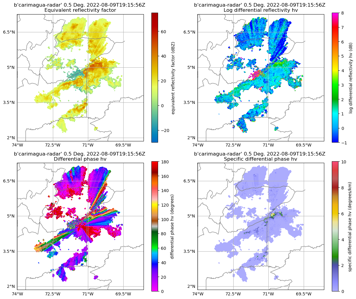

../../_images/cbb2d61a0c59a5a669e906517009a33c49af3019b80fce7d1f2f599544bdbccd.png

We can notice from the previous figure that this is a intense precipitation event in Colombia with reflectivity values up to +55 dBZ, big raindrops (\(Z_{DR}\) +3 dB), heavy rainfall rates with \(K_{DP}\) +10 dB/km, and multiples foldings in differential phase (\(Phi_{DP}\)). We can notice negative values in the \(Z_{DR}\) panel (differential attenuation) in the north-east side of the radar location.

\(K_{DP}\) retrieval methods

Although the radar data already contains the specific differential phase (\(K_{DP}\)), we can use the following alternative methods for comparison:

Variational method by Maesaka et al. (2012).
Kalman filter method by Schneebeli and al. (2014)
Vulpiani method by Vulpiani et al. (2012)

The Py-Art Python package includes all the methods mentioned above. We can access the retrieval methods using pyart.retrieve.kdp_maesaka, pyart.retrieve.kdp_schneebeli, and pyart.retrieve.kdp_vulpiani. The output from all retrieval methods is a tuple with two dictionaries that contain the retrieved \(K_{DP}\) as well as the Differential phase (\(Phi_{DP}\)).

%%time
kdp_maesaka= pyart.retrieve.kdp_maesaka(radar)

CPU times: user 6.34 s, sys: 10.2 s, total: 16.6 s
Wall time: 4.37 s

%%time
kdp_schneebeli = pyart.retrieve.kdp_schneebeli(radar, band='C', parallel=True)

CPU times: user 270 ms, sys: 393 ms, total: 663 ms
Wall time: 2min 38s

%%time
kdp_vulpiani = pyart.retrieve.kdp_vulpiani(radar, band='C', parallel=True)

CPU times: user 170 ms, sys: 271 ms, total: 440 ms
Wall time: 858 ms

This is how a dictionary with the retrieve \(K_{DP}\) looks like

kdp_vulpiani[0]

{'units': 'degrees/km',
 'standard_name': 'specific_differential_phase_hv',
 'long_name': 'Specific differential phase (KDP)',
 'coordinates': 'elevation azimuth range',
 'data': masked_array(
   data=[[0.0, 0.0, 0.0, ..., --, --, --],
         [0.0, 0.0, 0.0, ..., --, --, --],
         [0.0, 0.0, 0.0, ..., --, --, --],
         ...,
         [0.0, 0.0, 0.0, ..., --, --, --],
         [0.0, 0.0, 0.0, ..., --, --, --],
         [0.0, 0.0, 0.0, ..., --, --, --]],
   mask=[[False, False, False, ...,  True,  True,  True],
         [False, False, False, ...,  True,  True,  True],
         [False, False, False, ...,  True,  True,  True],
         ...,
         [False, False, False, ...,  True,  True,  True],
         [False, False, False, ...,  True,  True,  True],
         [False, False, False, ...,  True,  True,  True]],
   fill_value=-9999.0)}

Add the new retrieved \(K_{DP}\) values to the radar object

We can add new fields to our Py-Art radar object by using the pyart.core.Radar.add_field method as follows

radar.add_field('kdp_maesaka', kdp_maesaka[0])
radar.add_field('phidp_maesaka', kdp_maesaka[1])
radar.add_field('kdp_schneebeli', kdp_schneebeli[0])
radar.add_field('phidp_schneebeli', kdp_schneebeli[1])
radar.add_field('kdp_vulpiani', kdp_vulpiani[0])
radar.add_field('phidp_vulpiani', kdp_vulpiani[1])

List the new fields/variables

sorted(list(radar.fields))

['cross_correlation_ratio',
 'differential_phase',
 'differential_reflectivity',
 'kdp_maesaka',
 'kdp_schneebeli',
 'kdp_vulpiani',
 'normalized_coherent_power',
 'phidp_maesaka',
 'phidp_schneebeli',
 'phidp_vulpiani',
 'radar_echo_classification',
 'reflectivity',
 'specific_differential_phase',
 'spectrum_width',
 'total_power',
 'velocity']

Compare default and retrieved \(Phi_{DP}\) and \(K_{DP}\)

We can look at the difference between all the methods using a side-by-side comparison figure

# list of the variables to be plotted
vpol = ['specific_differential_phase', 'kdp_maesaka', 'kdp_schneebeli', 'kdp_vulpiani',
        'differential_phase', 'phidp_maesaka', 'phidp_schneebeli', 'phidp_vulpiani']
# list of cmaps
cmaps = ['pyart_Carbone42'] * 4 + ['pyart_Wild25'] * 4

# list of maximum values
vmaxs = [10] * 4 + [180]  * 4 

# list of tltles
titles = [r"$K_{DP} \ Default$", r"$K_{DP} \ Maesaka$", r"$K_{DP} \ Schneebeli$", r"$K_{DP} \ Vulpiani$", 
          r"$Phi_{DP} \ Default$", r"$Phi_{DP} \ Maesaka$", r"$Phi_{DP} \ Schneebeli$", r"$Phi_{DP} \ Vulpiani$"]

# display object from PyArt
display = pyart.graph.RadarMapDisplay(radar)
fig, axs = plt.subplots(2, 4, figsize=(14,6), subplot_kw={'projection': ccrs.PlateCarree()}, sharey=True, sharex=True)

# Extract the latitude and longitude of the radar and use it for the center of the map
lat_center = round(radar.latitude['data'][0], 0)
lon_center = round(radar.longitude['data'][0], 0)

# Set the projection - in this case, we use a general PlateCarree projection
projection = ccrs.PlateCarree()

# Determine the ticks
lat_ticks = np.arange(lat_center-3, lat_center+3, 1.5)
lon_ticks = np.arange(lon_center-3, lon_center+3, 1.5)

#make axis flatten for iteration
axis = axs.flatten()
# Loop to create all plots
for idx, ax in enumerate(axis):
    display.plot_ppi_map(vpol[idx], 0, resolution='10m', ax=ax, 
                         lat_lines=lat_ticks, 
                         lon_lines=lon_ticks,
                         cmap=cmaps[idx],
                         vmin=0, 
                         vmax=vmaxs[idx],
                         colorbar_flag=False, 
                         title_flag=False, 
                         add_grid_lines=False)
    ax.set_title(titles[idx])
    gl = ax.gridlines(draw_labels=True, rasterized=True)
    gl.xlocator = mticker.FixedLocator(lon_ticks)
    gl.ylabels_right = False
    gl.xlabels_top = False
    gl.ylabels_left = False
    gl.xlabels_bottom = False
    if (idx == 0) | (idx== 4):
        gl.ylabels_left = True
    if  idx>= 4:
        gl.xlabels_bottom = True

fig.tight_layout()
fig.colorbar(display.plots[0], ax=axis[:4], pad=.01, label='$Specific \ differential \  phase  \ [deg/km]$')
fig.colorbar(display.plots[-1], ax=axis[-4:], pad=.01, label='$Differential \ phase  \ [deg]$')
# fig.savefig('../images/kdp_comparison.jpg')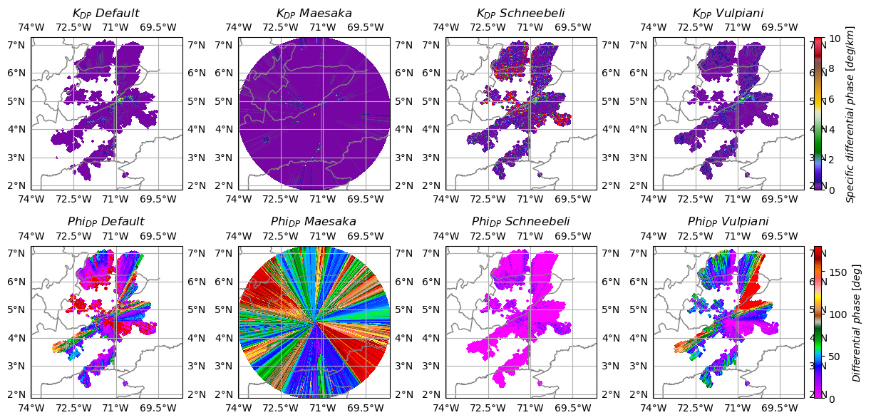

<matplotlib.colorbar.Colorbar at 0x7feca9f30d70>

../../_images/27c13cb2f6611353933a3a46849b13d616ae4282d3d376a817785c4691e80528.png

In the top row, we can see the Specific Differential Phase (\(K_{DP}\)), and in the bottom row, the Differential Phase (\(Phi_{DP}\)). We can notice that the default \(K_{DP}\) shows values +10 deg/km, which we think is too high. On the other hand, Maesake’s and Scneebeli’s methods’ output suggests that they are probably not performing well. However, the Vulpiani method performs better since we can observe more realistic values on \(K_{DP}\) and \(Phi_{DP}\).

Warning

This notebook is intended to be demonstrative; therefore, we can not make any conclusions regarding the methods we tested.

Summary

Within this example, we walked through how to access Colombian radar data from IDEAM, plot a quick look of the data, and compare the the specific differential phase using the default and three different methods!

What’s Next?

We will showcase other data workflow examples, including field campaigns in other regions and data access methods from other data centers.

Resources and References

IDEAM radar data
Py-ART:
- Helmus, J.J. & Collis, S.M., (2016). The Python ARM Radar Toolkit (Py-ART), a Library for Working with Weather Radar Data in the Python Programming Language. Journal of Open Research Software. 4(1), p.e25. DOI: http://doi.org/10.5334/jors.119
ACT:
- Adam Theisen, Ken Kehoe, Zach Sherman, Bobby Jackson, Alyssa Sockol, Corey Godine, Max Grover, Jason Hemedinger, Jenni Kyrouac, Maxwell Levin, Michael Giansiracusa (2022). The Atmospheric Data Community Toolkit (ACT). Zenodo. DOI: https://doi.org/10.5281/zenodo.6712343
Maesaka, T., Iwanami, K. and Maki, M., 2012: Non-negative KDP Estimation by Monotone Increasing PHIDP Assumption below Melting Layer. The Seventh European Conference on Radar in Meteorology and Hydrology.
Schneebeli, M., Grazioli, J., and Berne, A., 2014: Improved Estimation of the Specific Differential Phase SHIFT Using a Compilation of Kalman Filter Ensembles, IEEE T. Geosci. Remote Sens., 52, 5137-5149, https://doi:10.1109/TGRS.2013.2287017
Gianfranco Vulpiani, Mario Montopoli, Luca Delli Passeri, Antonio G. Gioia, Pietro Giordano, and Frank S. Marzano, 2012: On the Use of Dual-Polarized C-Band Radar for Operational Rainfall Retrieval in Mountainous Areas. J. Appl. Meteor. Climatol., 51, 405-425, doi: https://10.1175/JAMC-D-10-05024.1.