Buoys and Wave(let)s
Overview
Generating a wavelet power spectrum from the time-series data of wave heights collected from buoy station 44013 east of Boston
Prerequisties
Background
Download and Organize Buoy Data
Wavelet Input Values
PyWavelets
Power Spectrum
Prerequisites
| Concepts | Importance | Notes |
|---|---|---|
| Intro to Matplotlib | Necessary | Used to plot data |
| Intro to Numpy | Necessary | Used to work with large arrays |
| Intro to Datetimes | Helpful | Useful to understand strings vs. datetimes |
Time to learn: 35 minutes
Background
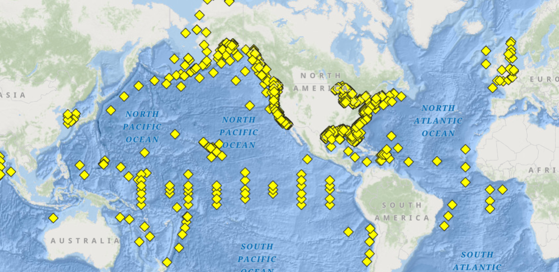
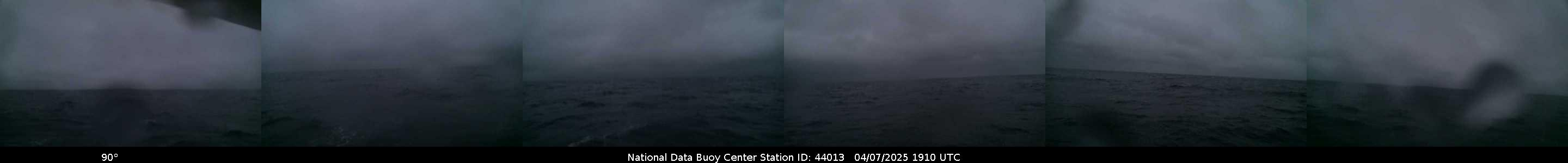
Buoys float on the surface of water, and while they can serve many purposes, research facilities like NOAA’s National Data Buoy Center provide real-time and historical data about waves and climate on the ocean and within lakes from hundreds of buoys around the world.
Each buoy has been in service for a variety of years and collects different information. Buoy 44013 is off the coast of Boston in the Massachusetts Bay and reports information about the wind speed and direction, atmospheric pressure, air temperature, dew point, water temperature, and wave height throughout the year.
| Location | Buoy |
|---|---|
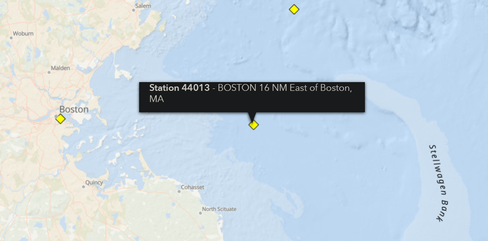 |  |
44013 is owned and operated by the National Data Buoy Center and measures a depth of 64.6 meters and has a watch circle radius of 122 yards, with standard meterological data dating back to 1984.
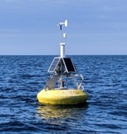
Example Buoy Camera Photos from April 7, 2025:
And a photo from today:

For this notebook, we will be investigating the wave height of the buoy across two years in the early 2000’s
Imports
import numpy as np                          # working with arrays
import matplotlib.pyplot as plt             # plot data
import datetime                             # converting strings to datetime objects
import requests                             # retrieve data from text on a website

import pywt                                 # PyWavelets
Access Buoy Data
First, we will need to download the relevant data from NOAA National Data Buoy Center. For this notebook, we will be investigating wave height data from 2001 to 2002.
The buoy contains more information than just wave height, so we will save only data relevant to the date and time and the wave height. So, the columns we need to keep are date, time (YY, MM, DD, hh), and wave height (WVHT).
We will iterate through the years to save and concatenate the data into a single large array.
years = [2001, 2002]
date_times = np.array([])
wave_height = np.array([])
for i, year in enumerate(years):

    # collect data from NOAA Buoy link
    data_link = f"https://www.ndbc.noaa.gov/view_text_file.php?filename=41001h{year}.txt.gz&dir=data/historical/stdmet/"
    data_req = requests.get(data_link)
    data_txt = data_req.text
    data = np.genfromtxt(data_txt.splitlines(), comments=None, dtype='str')

    # Find the index for datetime and wave height information
    datetime_index = np.where(data[0] == "hh")[0][0]
    wave_height_index = np.where(data[0] == "WVHT")[0][0]

    # collect data from all rows for the columns of datetime and wave height
    # [1:] skips the first row with header information
    date_time = data[:,:datetime_index+1][1:]
    data_wave_height = data[:,wave_height_index][1:]

    # Converts the string data collected from the source to a float
    data_wave_height = data_wave_height.astype(float)

    # Concatenate all data into a single array
    if i == 0:
        date_times = date_time
        wave_height = data_wave_height
    else:
        date_times = np.concatenate([date_times, date_time])
        wave_height = np.concatenate([wave_height, data_wave_height])
Clean Up Wave Height data
Buoys stores null as 99.00, so to remove this outlier, we will need to replace 99.00 with np.nan.
print(f"Max wave height before applying nan = {max(wave_height)} m")
wave_height = np.where(wave_height == 99.00, np.nan, wave_height)
print(f"Max wave height after applying nan  = {max(wave_height)} m")
Max wave height before applying nan = 99.0 m
Max wave height after applying nan = 9.38 m
Convert Time to Datetimes
Buoys store datetime information as separate columns of data with YYYY MM DD and HH. For Python to recognize these strings as a date, we need to combine the strings into a single datetime value.
dates = []
for date in date_times:
    # combine each separate column into a single string: YYYYMMDDHH
    date_string = "".join(date)
    # convert string to a datetime object
    dates.append(datetime.datetime.strptime(date_string, "%Y%m%d%H"))
dates = np.array(dates)
print(f"First Date = {dates[0]}")
print(f"Last Date  = {dates[-1]}")
First Date = 2001-01-01 00:00:00
Last Date = 2002-12-17 20:00:00
Plot and View Data
Let’s give the data a look! Wave height is recorded in meters throughout the year.
fig, ax = plt.subplots(figsize=(10, 10))
plt.title("Wave Height on Station 44013")
plt.xlabel("Date")
plt.xticks(rotation=90)
plt.ylabel("Wave Height (meters)")
plt.plot(dates, wave_height)
plt.show()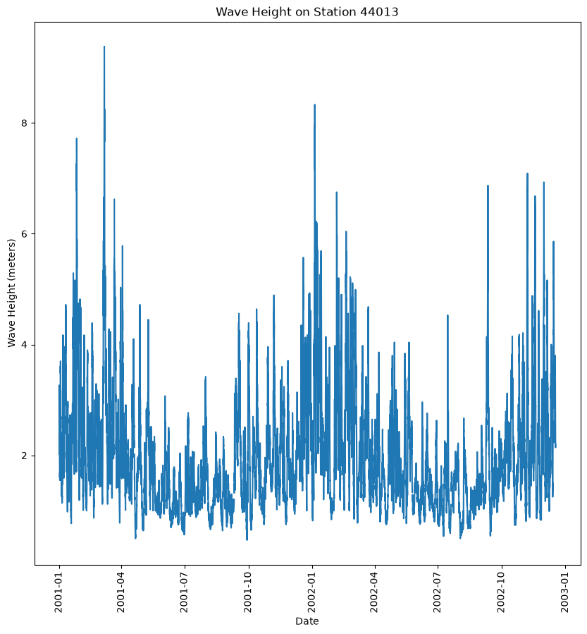
Wavelet Input Values
Wavelet inputs include:
x: Input time-series data (for example, the time and wave height of data)
wavelet: mother wavelet name
dt: sampling period (time between each y-value) for time range
s0: smallest scale
dj: spacing between each discrete scales
jtot: largest scale
dt = 3600   # sampling period (time between each y-value) ->  seconds in an hour
s0 = 0.25   # smallest scale
dj = 0.25   # spacing between each discrete scales
jtot = 64   # largest scale
For this example, we will be using a complex Morlet with a bandwidth of 1.5 and a center frequency of 1.
bandwidth = 1.5
center_freq = 1
wavelet_mother = f"cmor{bandwidth}-{center_freq}"
print(wavelet_mother)
cmor1.5-1
Applying Wavelets
scales = np.arange(1, jtot + 1, dj)
wavelet_coeffs, freqs = pywt.cwt(
    data=wave_height, scales=scales, wavelet=wavelet_mother, sampling_period=dt
)
Power Spectrum
The power spectrum is the real component of the wavelet coefficients. We can find this value by squaring the absolute value of the wavelet_coeffs to return the magnitude of the real component to make a better graph.
power = np.power((abs(wavelet_coeffs)), 2)

fig, ax = plt.subplots(figsize=(10, 10))

# Plot Scalogram
plt.imshow(
    power, vmax=(power).max(), vmin=(power).min(), aspect="auto"
)

# Plot X-Axis with Date Labels and Ticks Monthly
num = 730 # hours in a month
x_ticks = range(0, len(dates), num)
x_ticklabels = []
for date in dates[::num]:
    x_ticklabels.append(str(date)[:-9])
plt.xticks(ticks=x_ticks, labels=x_ticklabels,rotation=90)

plt.title("Buoy Height at Station 44013")
plt.xlabel("Date (Hours)")
plt.ylabel("Scale")
plt.colorbar()
plt.show()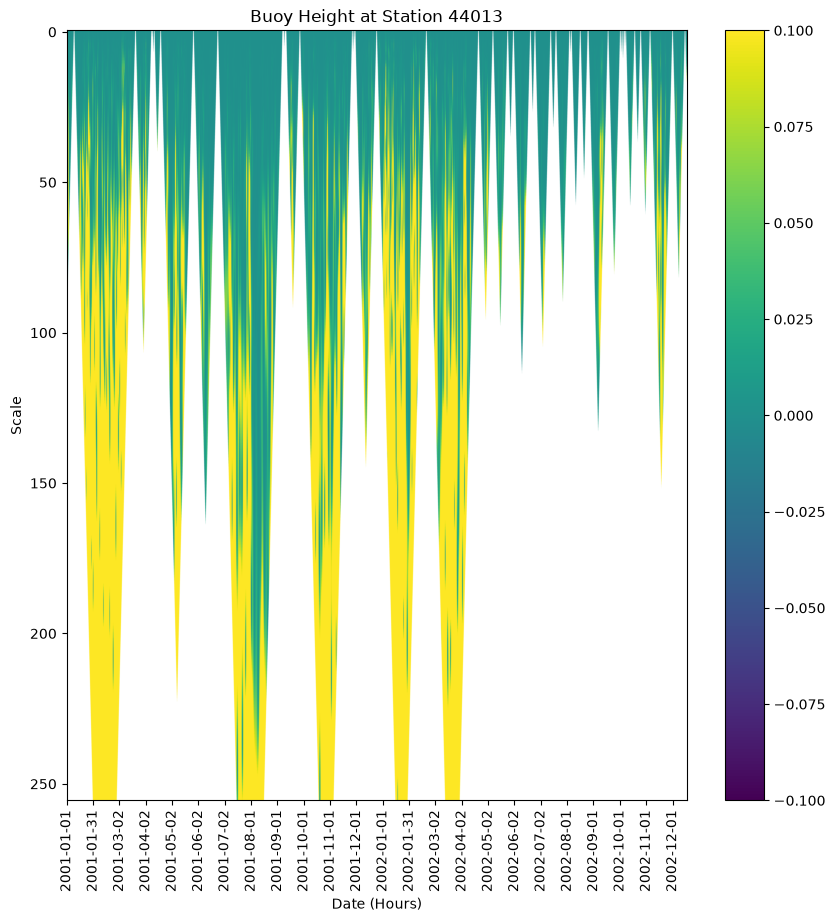
What Went Wrong?
The current wavelet has a lot of blank space that is confusing the wavelet analysis. This is the result of the nan values, where data was no included, but is still being used in the calculation. So, to get a complete wavelet, we should filter out the nan values before we apply a wavelet.
We will fix this by applying a mask to all the nan values, and then interpolating between to fill out the remaining data.
wave_len = np.arange(len(wave_height))
mask = np.isfinite(wave_height)
xfiltered = np.interp(wave_len, wave_len[mask], wave_height[mask])
Time to get our wavelet_coeffs from the newly filtered data.
scales = np.arange(1, jtot + 1, dj)
wavelet_coeffs, freqs = pywt.cwt(
    data=xfiltered, scales=scales, wavelet=wavelet_mother, sampling_period=dt
)
Power Spectrum, Take Two
power = np.power((abs(wavelet_coeffs)), 2)

fig, ax = plt.subplots(figsize=(10, 10))

# Plot Scalogram
plt.imshow(
    power, vmax=(power).max(), vmin=(power).min(), aspect="auto"
)

# Plot X-Axis with Date Labels and Ticks Monthly
num = 730 # hours in a month
x_ticks = range(0, len(dates), num)
x_ticklabels = []
for date in dates[::num]:
    x_ticklabels.append(str(date)[:-9])
plt.xticks(ticks=x_ticks, labels=x_ticklabels,rotation=90)

plt.title("Buoy Height at Station 44013")
plt.xlabel("Date (Hours)")
plt.ylabel("Scale")
plt.colorbar()
plt.show()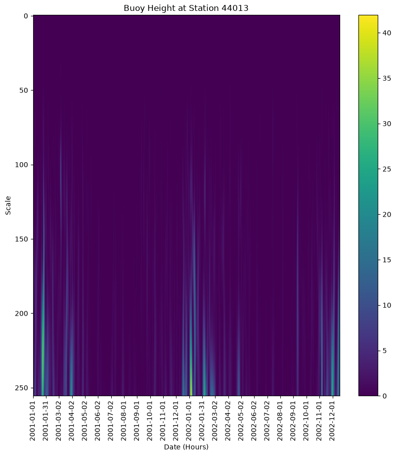
That’s more like it!
Now, the x-axis describes the when and the y-axis describes the what
X axis describes when wind is present and causing waves
Y axis describes the range of wave periods needed to make the signal that is present. There is a large range when waves are detected, which is expected since wind excites many frequencies of waves on the surface when it blows
Conclusions
The power spectrum above demonstrates a strong peak (in yellow) within the first month of the year. During this time of year, the wave activity is high and across a wide range of frequencies. This wavelet is demonstrating when wave activity is highest and the range of wave heights is widest.
Summary
Wavelet analysis can be applied across a wide range of data, as long as there is a time-series data. Buoys returns a large range of possible data, but for this example we explored how wave heights vary throughout the year. There is a large amount of wave activity in very short intervals at the beginning of the year, but the wave heights vary over a large range of possible frequencies.