Weekly Sea Surface Temperature Patterns from NOAA

Atmospheric Data: Nino 3 SST Index¶

Overview¶

Generating a wavelet power and phase spectrum from the time-series data Nino 3 SST Index

Prerequisties
Background
Download and Organize Nino 3 SST Data
Wavelet Input Values
PyWavelets
Power Spectrum
Phase Spectrum

Prerequisites¶

Concepts	Importance	Notes
Intro to Matplotlib	Necessary	Used to plot data
Intro to Pandas	Necessary	Used to read in and organize data (in particular dataframes)
Intro to Numpy	Necessary	Used to work with large arrays
Intro to SciPy	Helpful	Used to work with .wav files and built-in Fast Fourier Transform

Time to learn: 45 minutes

Background¶

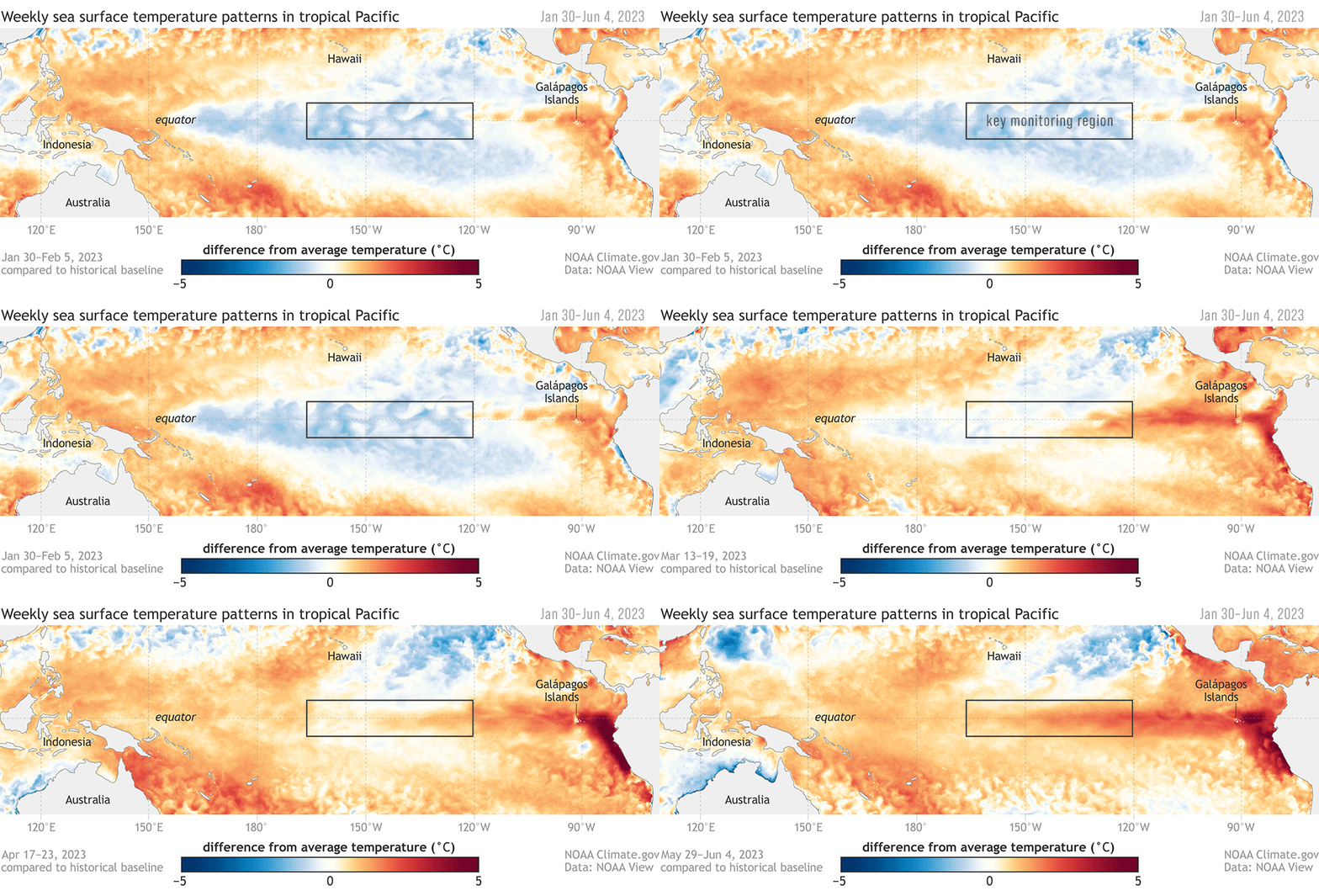
What is an El Niño?¶

Learn more!

Wavelets and Atmospheric Data¶

Weather is a great example of time-series data. Weather varies in cycles of temperature over weeks due to a huge number of variables. Wavelet analysis can be used to find patterns in temperature by analyzing both the temperature and the time when the temperature occurs.

Imports¶

import geocat.datafiles as gcd              # accessing nino3 data file
import xarray as xr                         # working with geocat-datafiles

import numpy as np                          # working with arrays
import pandas as pd                         # working with dataframes
import matplotlib.pyplot as plt             # plot data

import pywt                                 # PyWavelets

Downloading file 'registry.txt' from 'https://github.com/NCAR/geocat-datafiles/raw/main/registry.txt' to '/home/runner/.cache/geocat'.

Download Nino 3 SST Data¶

We will be downloading the sst_nino3 data from geocat-datafiles

nino3_data = gcd.get('ascii_files/sst_nino3.dat')
nino3_data = np.loadtxt(nino3_data)

Downloading file 'ascii_files/sst_nino3.dat' from 'https://github.com/NCAR/geocat-datafiles/raw/main/ascii_files/sst_nino3.dat' to '/home/runner/.cache/geocat'.

Plot and View Data¶

Let’s give the data a look! We have over a hundred years worth of temperature readings.

fig, ax = plt.subplots(figsize=(8, 8))
plt.title("El Niño Sea Surface Temperature")
plt.xlabel("Years (from 1871)")
plt.ylabel("Sea Surface Temparture Changes")
plt.plot(nino3_data)
plt.show()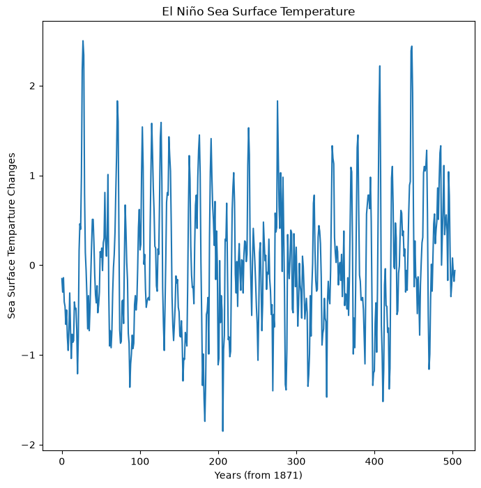

Update the X-Axis¶

By default, the loaded data lists the year as time since 1871, we can add a new x-axis to view the years along the x-axis

# Convert default X-axis from time steps of 0-504 (0-len(nino3_data)) to Years
dt = 0.25  # sampling period
start_year = 1871
end_year = 1871 + (len(nino3_data) * dt)
x_tickrange = np.arange(start_year, end_year, dt)
start = int(9 / dt)  # 36, starts the x-axis label at 1880 (9 years after start of data)
display_nth = int(20 / dt)  # 80, display x-axis label every 20 years

fig, ax = plt.subplots(figsize=(8, 8))
plt.title("El Niño Sea Surface Temperature")
plt.xlabel("Year")
plt.ylabel("Sea Surface Temparture Changes")
plt.xticks(range(len(x_tickrange))[start::display_nth], x_tickrange[start::display_nth]) # update x-axis
plt.plot(nino3_data)
plt.show()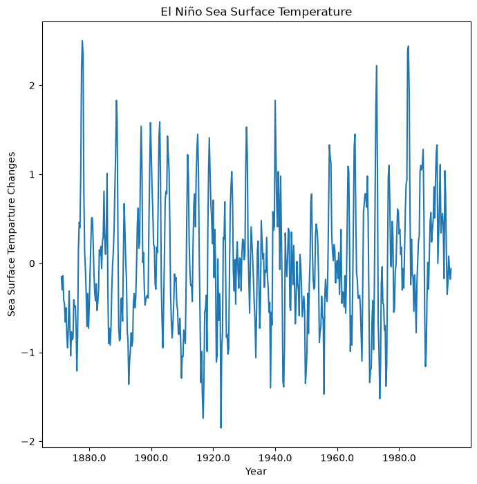

Wavelet Input Values¶

Wavelet inputs include:

x: Input time-series data (for example, the time and temperature data from nino3)
wavelet: mother wavelet name
dt: sampling period (time between each y-value)
s0: smallest scale
dj: spacing between each discrete scales
jtot: largest scale

dt = 0.25  # sampling period (time between each y-value)
s0 = 0.25  # smallest scale
dj = 0.25  # spacing between each discrete scales
jtot = 64  # largest scale

Define Complex Morlet¶

A complex Morlet allows us to define both the bandwidth and the center frequency that the Morlet wavelet will be built from to produce optimal results.

Here you can learn more about how PyWavelets configures Complex Morlet wavelets

Below you can see how changing the bandwidth and center frequency will change how the mother Complex Morlet wavelet’s shape is formed. The shape of the wavelet will impact which frequencies it is sensitive to.

wavelets = [f"cmor{x:.1f}-{y:.1f}" for x in [0.5, 1.5, 2.5] for y in [0.5, 1.0, 1.5]]
fig, axs = plt.subplots(3, 3, figsize=(10, 10), sharex=True, sharey=True)
for ax, wavelet in zip(axs.flatten(), wavelets):
    [psi, x] = pywt.ContinuousWavelet(wavelet).wavefun(10)
    ax.plot(x, np.real(psi), label="real")
    ax.plot(x, np.imag(psi), label="imag")
    ax.set_title(wavelet)
    ax.set_xlim([-5, 5])
    ax.set_ylim([-0.8, 1])
ax.legend()
plt.suptitle("Complex Morlet Wavelets with different center frequencies and bandwidths from PyWavelets")
plt.show()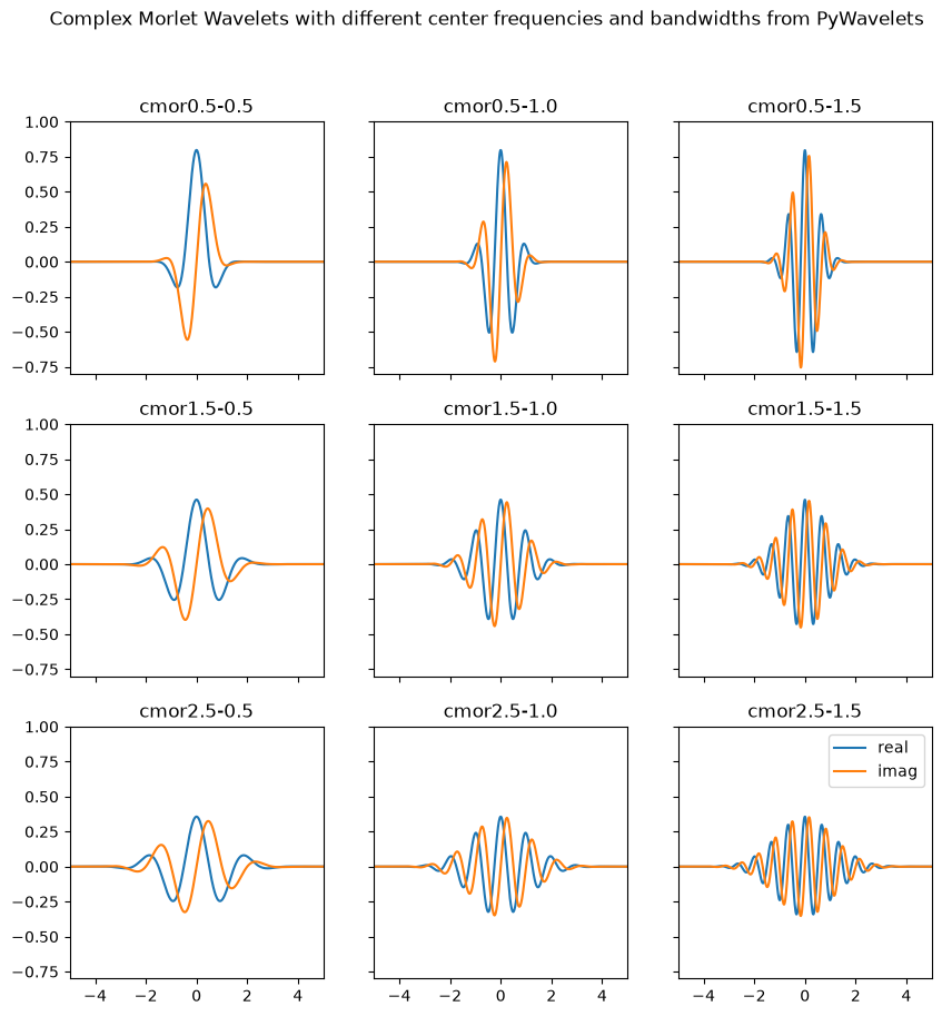

Changing the bandwidth and center frequency can be a useful tool to optimize how well the mother wavelet will be able to find frequencies in the data.

Below you will see how different values for bandwidth and center frequency can lead to greater or poorer resolution of the same signal.

# Code below from: https://pywavelets.readthedocs.io/en/latest/ref/cwt.html

def gaussian(x, x0, sigma):
    return np.exp(-np.power((x - x0) / sigma, 2.0) / 2.0)


def make_chirp(t, t0, a):
    frequency = (a * (t + t0)) ** 2
    chirp = np.sin(2 * np.pi * frequency * t)
    return chirp, frequency


def plot_wavelet(time, data, wavelet, title, ax):
    widths = np.geomspace(1, 1024, num=75)
    cwtmatr, freqs = pywt.cwt(
        data, widths, wavelet, sampling_period=np.diff(time).mean()
    )
    cwtmatr = np.abs(cwtmatr[:-1, :-1])
    pcm = ax.pcolormesh(time, freqs, cwtmatr)
    ax.set_yscale("log")
    ax.set_xlabel("Time (s)")
    ax.set_ylabel("Frequency (Hz)")
    ax.set_title(title)
    plt.colorbar(pcm, ax=ax)
    return ax

# generate signal
time = np.linspace(0, 1, 1000)
chirp1, frequency1 = make_chirp(time, 0.2, 9)
chirp2, frequency2 = make_chirp(time, 0.1, 5)
chirp = chirp1 + 0.6 * chirp2
chirp *= gaussian(time, 0.5, 0.2)

# perform CWT with different wavelets on same signal and plot results
wavelets = [f"cmor{x:.1f}-{y:.1f}" for x in [0.5, 1.5, 2.5] for y in [0.5, 1.0, 1.5]]
fig, axs = plt.subplots(3, 3, figsize=(10, 10), sharex=True)
for ax, wavelet in zip(axs.flatten(), wavelets):
    plot_wavelet(time, chirp, wavelet, wavelet, ax)
plt.tight_layout(rect=[0, 0.03, 1, 0.95])
plt.suptitle("Scalograms of the same signal with different wavelets")
plt.show()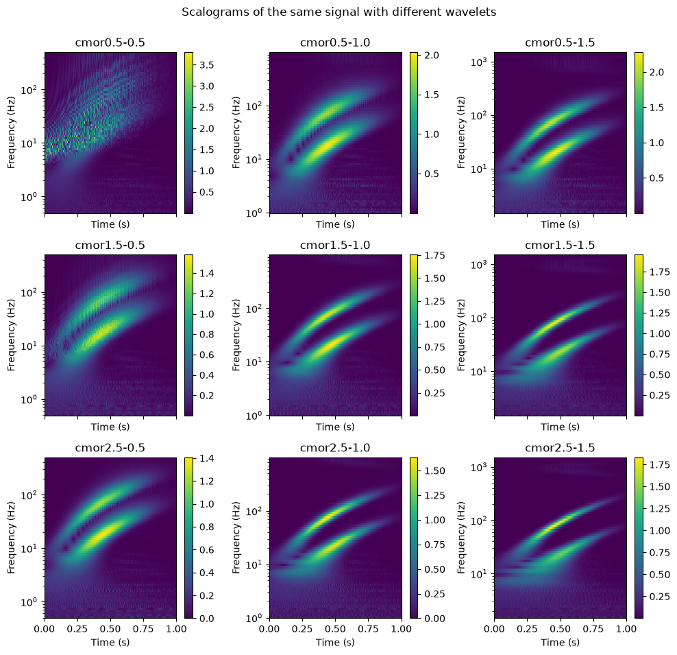

For this example, we will be using a complex Morlet with a bandwidth of 1.5 and a center frequency of 1

bandwidth = 1.5
center_freq = 1
wavelet_mother = f"cmor{bandwidth}-{center_freq}"
print(wavelet_mother)

cmor1.5-1

Applying Wavelets¶

scales = np.arange(1, jtot + 1, dj)
wavelet_coeffs, freqs = pywt.cwt(
    data=nino3_data, scales=scales, wavelet=wavelet_mother, sampling_period=dt
)

Power Spectrum¶

The power spectrum is the real component of the wavelet coefficients. We can find this value by squaring the absolute value of the wavelet_coeffs to return the magnitude of the real component to make a better graph.

power = np.power((abs(wavelet_coeffs)), 2)

fig, ax = plt.subplots(figsize=(10, 10))

# Plot contour around data
plt.contour(
    power, vmax=(power).max(), vmin=(power).min(), levels=10
)
plt.contour(power, levels=10, colors="k", linewidths=0.5, alpha=0.75)

# Plot Scalogram
plt.imshow(
    power, vmax=(power).max(), vmin=(power).min(), aspect="auto"
)

plt.xticks(range(len(x_tickrange))[start::display_nth], x_tickrange[start::display_nth])
plt.title("El Niño Wavelet Power Spectrum")
plt.xlabel("Year")
plt.ylabel("Scale")
plt.colorbar()
plt.show()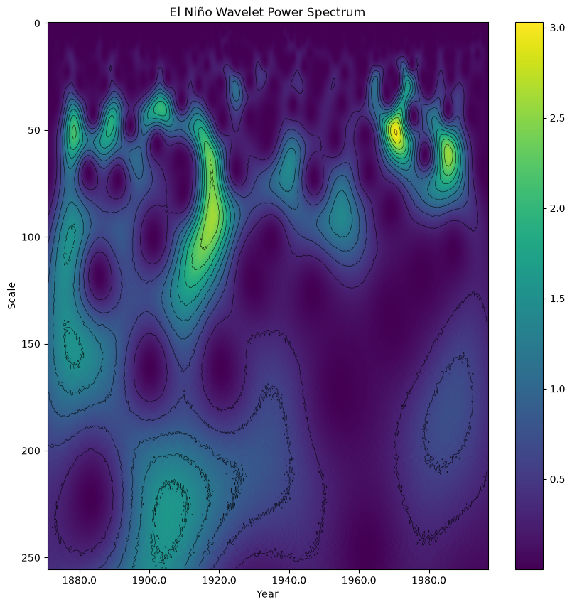

The power spectrum above demonstrates a strong peak (in yellow) at 50 that represents an interesting consistent pattern across the decades of atmosphere data.

Phase Spectrum¶

While less commonly used, the phase spectrum is the imaginary component of the wavelet.

# compare the phase spectrum
phase = np.angle(wavelet_coeffs)

fig, ax = plt.subplots(figsize=(10, 10))

# Convert Y-Axis from default to symmetrical log (symlog) with labels
ax.set_yscale("symlog")
ax.invert_yaxis()
ax.set_yticks([10, 20, 30, 40, 50])
ax.set_yticklabels([10, 20, 30, 40, 50])

# Plot scalogram
plt.imshow(
    phase, vmax=(phase).max(), vmin=(phase).min(), aspect="auto"
)

# Convert default X-axis from time steps of 0-504 (0-len(sst_data)) to Years
start_year = 1871
end_year = 1871 + (len(nino3_data) * dt)
x_tickrange = np.arange(start_year, end_year, dt)
start = int(9 / dt)  # 36, starts the x-axis label at 1880 (9 years after start of data)
display_nth = int(20 / dt)  # 80, display x-axis label every 20 years
plt.xticks(range(len(x_tickrange))[start::display_nth], x_tickrange[start::display_nth])

plt.title("El Niño Wavelet Phase Spectrum")
plt.xlabel("Year")
plt.ylabel("Scale")
plt.colorbar()
plt.show()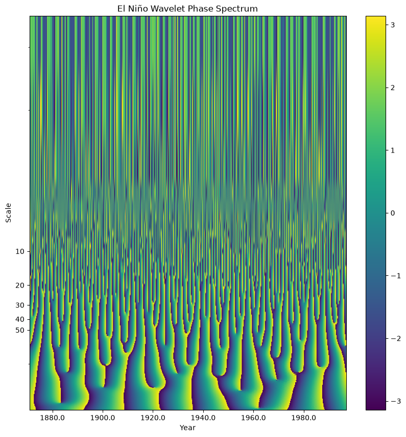

Summary¶

Frequency signals appear in more than just audio! A frequency analysis of weather data can inform us about how weather trends change through a year and over a decades worth of data.

What’s next?¶

Buoys and Wave(lets)

Resources and references¶

“A Practical Guide to Wavelet Analysis” (Torrence and Compo, 1998)