Let’s start here! If you can directly link to an image relevant to your notebook, such as canonical logos, do so here at the top of your notebook. You can do this with Markdown syntax,

![<image title>](http://link.com/to/image.png "image alt text")

or edit this cell to see raw HTML img demonstration. This is preferred if you need to shrink your embedded image. Either way be sure to include alt text for any embedded images to make your content more accessible.

Making Plots using Stage IV Data

Next, title your notebook appropriately with a top-level Markdown header, #. Do not use this level header anywhere else in the notebook. Our book build process will use this title in the navbar, table of contents, etc. Keep it short, keep it descriptive. Follow this with a --- cell to visually distinguish the transition to the prerequisites section.

---

Overview

Good morning, world! If you have an introductory paragraph, lead with it here! Keep it short and tied to your material, then be sure to continue into the required list of topics below,

1. This is a numbered list of the specific topics

2. These should map approximately to your main sections of content

3. Or each second-level, ##, header in your notebook

4. Keep the size and scope of your notebook in check

5. And be sure to let the reader know up front the important concepts they’ll be leaving with

Prerequisites

This section was inspired by this template of the wonderful The Turing Way Jupyter Book.

Following your overview, tell your reader what concepts, packages, or other background information they’ll need before learning your material. Tie this explicitly with links to other pages here in Foundations or to relevant external resources. Remove this body text, then populate the Markdown table, denoted in this cell with | vertical brackets, below, and fill out the information following. In this table, lay out prerequisite concepts by explicitly linking to other Foundations material or external resources, or describe generally helpful concepts.

Label the importance of each concept explicitly as helpful/necessary.

Concepts	Importance	Notes
Intro to Cartopy	Necessary
Understanding of NetCDF	Helpful	Familiarity with metadata structure
Project management	Helpful

• Time to learn: estimate in minutes. For a rough idea, use 5 mins per subsection, 10 if longer; add these up for a total. Safer to round up and overestimate.

• System requirements:

  • Populate with any system, version, or non-Python software requirements if necessary

  • Otherwise use the concepts table above and the Imports section below to describe required packages as necessary

  • If no extra requirements, remove the System requirements point altogether

---

Imports

Begin your body of content with another --- divider before continuing into this section, then remove this body text and populate the following code cell with all necessary Python imports up-front:

import fsspec
import numpy as np
import xarray as xr
import pandas as pd
import cartopy.crs as ccrs
import cartopy.feature as cfeature
from matplotlib import pyplot as plt
from matplotlib.dates import DateFormatter, AutoDateLocator,HourLocator,DayLocator
from datetime import datetime, timedelta
from metpy.plots import USCOUNTIES
import matplotlib.colors as colors
from pyproj import Proj
import seaborn as sns
sns.set()

CONUS Plots of Stage IV Data

Load in the data!

zarr_url = f's3://mdmf/gdp/stageiv_combined.zarr/'

fs2 = fsspec.filesystem('s3', anon=True, endpoint_url='https://usgs.osn.mghpcc.org/')

ds = xr.open_dataset(fs2.get_mapper(zarr_url), engine='zarr',

                             backend_kwargs={'consolidated':True}, chunks={})

ds = ds.sortby('time')

precipitation_data = ds['Total_precipitation_surface_1_Hour_Accumulation']

precipitation_data.sel(time='2018-01-09 11:00').plot()

#precipitation_data.sortby('time').sel(time='2018-01-09 11:00').plot()

<matplotlib.collections.QuadMesh at 0x7fdc57d22190>

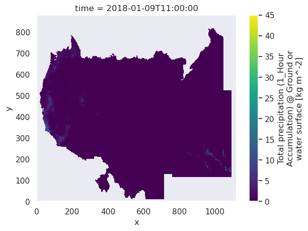
This basic plots shows: x/y grid points, the unit of km/m^-2)

We are using datetime.

A content subsection

Divide and conquer your objectives with Markdown subsections, which will populate the helpful navbar in Jupyter Lab and here on the Jupyter Book!

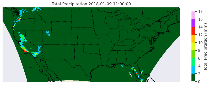
# Extract the relevant time range
start_time = '2018-01-09 11:00:00'
end_time = '2018-01-09 11:00:00'

precipitation_data = ds['Total_precipitation_surface_1_Hour_Accumulation'].sel(time=slice(start_time, end_time))

# Sum the precipitation values over the specified time range
total_precipitation = precipitation_data.sum(dim='time')

lon = ds['lon'].values
lat = ds['lat'].values

# Transpose the total_precipitation array if needed
total_precipitation = total_precipitation.transpose()

# Create a larger figure with Cartopy
fig, ax = plt.subplots(figsize=(12, 8), subplot_kw={'projection': ccrs.PlateCarree()})
ax.set_extent([-128, -66.5, 24, 50], crs=ccrs.PlateCarree())

# Add map features
ax.add_feature(cfeature.COASTLINE)
ax.add_feature(cfeature.BORDERS, linestyle=':')
ax.add_feature(cfeature.STATES, linestyle=':')
ax.add_feature(cfeature.LAND, edgecolor='black')

# Plot the total precipitation on the map
c = ax.contourf(lon, lat, total_precipitation, cmap='gist_ncar', levels=np.arange(0,20,2), extend='max', transform=ccrs.PlateCarree())
colorbar = plt.colorbar(c, ax=ax, label='Total Precipitation (mm)', shrink=0.5)  # Adjust the shrink parameter as needed

# Add title and labels
#plt.title('Total Precipitation from {} to {}'.format(start_time, end_time))
plt.title('Total Precipitation {}'.format(start_time))
plt.xlabel('Longitude')
plt.ylabel('Latitude')

# Show the plot
plt.show()

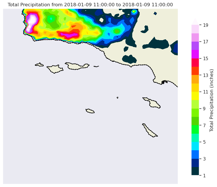
fig, ax = plt.subplots(figsize=(12, 8), subplot_kw={'projection': ccrs.PlateCarree()})
ax.set_extent([-121, -118, 32, 35], crs=ccrs.PlateCarree())

# Add map features
ax.add_feature(cfeature.COASTLINE)
ax.add_feature(cfeature.BORDERS, linestyle=':')
ax.add_feature(cfeature.STATES, linestyle=':', linewidth=2)
ax.add_feature(cfeature.LAND, edgecolor='black')

# Plot the total precipitation on the map   (levels=range(1,10) OR WHAT I HAVE NOW
c = ax.contourf(lon, lat, total_precipitation, cmap='gist_ncar', levels=np.arange(1, 20, 1), extend='max', transform=ccrs.PlateCarree())
colorbar = plt.colorbar(c, ax=ax, label='Total Precipitation (inches)', shrink=0.9)  # Adjust the shrink parameter as needed

# Add title and labels
plt.title('Total Precipitation from {} to {}'.format(start_time, end_time))
plt.xlabel('Longitude')
plt.ylabel('Latitude')

# Show the plot
plt.show()

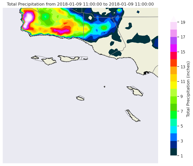
fig, ax = plt.subplots(figsize=(12, 8), subplot_kw={'projection': ccrs.PlateCarree()})
ax.set_extent([-121, -118, 32, 35], crs=ccrs.PlateCarree())

# Add map features
ax.add_feature(cfeature.COASTLINE)
ax.add_feature(cfeature.BORDERS, linestyle=':')
ax.add_feature(cfeature.STATES, linestyle=':', linewidth=2)
ax.add_feature(cfeature.LAND, edgecolor='black')
ax.add_feature(USCOUNTIES,edgecolor='grey', linewidth=1)

# Plot the total precipitation on the map   (levels=range(1,10) OR WHAT I HAVE NOW
c = ax.contourf(lon, lat, total_precipitation, cmap='gist_ncar', levels=np.arange(1, 20, 1), extend='max', transform=ccrs.PlateCarree())
colorbar = plt.colorbar(c, ax=ax, label='Total Precipitation (inches)', shrink=0.9)  # Adjust the shrink parameter as needed

# Add title and labels
plt.title('Total Precipitation from {} to {}'.format(start_time, end_time))
plt.xlabel('Longitude')
plt.ylabel('Latitude')

# Show the plot
plt.show()

Another content subsection

Keep up the good work! A note, try to avoid using code comments as narrative, and instead let them only exist as brief clarifications where necessary.

Your second content section

Here we can move on to our second objective, and we can demonstrate

Subsection to the second section

a quick demonstration

of further and further

header levels

as well \(m = a * t / h\) text! Similarly, you have access to other \(\LaTeX\) equation functionality via MathJax (demo below from link),

(1)\[\begin{align} \dot{x} & = \sigma(y-x) \\ \dot{y} & = \rho x - y - xz \\ \dot{z} & = -\beta z + xy \end{align}\]

Check out any number of helpful Markdown resources for further customizing your notebooks and the Jupyter docs for Jupyter-specific formatting information. Don’t hesitate to ask questions if you have problems getting it to look just right.

Last Section

If you’re comfortable, and as we briefly used for our embedded logo up top, you can embed raw html into Jupyter Markdown cells (edit to see):

Info

Your relevant information here!

Feel free to copy this around and edit or play around with yourself. Some other admonitions you can put in:

Success

We got this done after all!

Warning

Be careful!

Danger

Scary stuff be here.

We also suggest checking out Jupyter Book’s brief demonstration on adding cell tags to your cells in Jupyter Notebook, Lab, or manually. Using these cell tags can allow you to customize how your code content is displayed and even demonstrate errors without altogether crashing our loyal army of machines!

---

Summary

Add one final --- marking the end of your body of content, and then conclude with a brief single paragraph summarizing at a high level the key pieces that were learned and how they tied to your objectives. Look to reiterate what the most important takeaways were.

What’s next?

Let Jupyter book tie this to the next (sequential) piece of content that people could move on to down below and in the sidebar. However, if this page uniquely enables your reader to tackle other nonsequential concepts throughout this book, or even external content, link to it here!

Resources and references

Finally, be rigorous in your citations and references as necessary. Give credit where credit is due. Also, feel free to link to relevant external material, further reading, documentation, etc. Then you’re done! Give yourself a quick review, a high five, and send us a pull request. A few final notes:

• Kernel > Restart Kernel and Run All Cells... to confirm that your notebook will cleanly run from start to finish

• Kernel > Restart Kernel and Clear All Outputs... before committing your notebook, our machines will do the heavy lifting

• Take credit! Provide author contact information if you’d like; if so, consider adding information here at the bottom of your notebook

• Give credit! Attribute appropriate authorship for referenced code, information, images, etc.

• Only include what you’re legally allowed: no copyright infringement or plagiarism

Thank you for your contribution!