Loading and Visualizing Raster Data - Project Pythia Geomorphology Cookbook

Every analysis in this cookbook starts from a bathymetry grid stored as a GeoTIFF file. Before we can compute terrain derivatives or map seabed features, we need to read that file into Python, understand how its pixels relate to real-world positions, and display it. The library that does this is rasterio.

This notebook is a practical introduction to rasterio. It covers opening a raster, reading its metadata, pulling the pixel values into a NumPy array, and converting between pixel and map coordinates. For visualization it then hands off to the modern raster stack, rioxarray and xarray-spatial, so you never have to hand-write terrain math.

Overview¶

Reading band values into a NumPy array, including nodata handling.
Converting between pixel indices and map coordinates.
Visualizing a raster with rioxarray and xarray-spatial, then overlaying a semi-transparent hillshade for relief.
A reusable function for loading and visualizing bathymetric geotiffs.

Prerequisites¶

Concepts	Importance	Notes
NumPy arrays	Necessary	Raster bands are NumPy arrays
Matplotlib	Helpful	Used for all plots
Coordinate reference systems	Helpful	Rasters carry a CRS and a transform
Seabed Morphology	Helpful	Why bathymetry grids matter here

Time to learn: 30 minutes

Imports¶

from pathlib import Path

import numpy as np
import matplotlib.pyplot as plt
import matplotlib.ticker as mticker

import rasterio

# rioxarray registers the .rio accessor on xarray objects when imported
import rioxarray
from xrspatial import hillshade

# Tick formatter without scientific notation
formatter = mticker.FuncFormatter(lambda x, pos: f"{int(x):,}")

Visualizing a raster¶

You could plot the array straight from rasterio with imshow, but then the axes are in pixel indices, not map coordinates, and you would have to build a hillshade by hand. The modern approach is to load the same file with rioxarray, which returns an xarray.DataArray that carries the coordinates and CRS with it. Labelled plotting and terrain shading then come for free.

open_rasterio returns a DataArray with a leading band dimension; squeeze drops it for our single-band file, and masked=True applies the nodata mask as NaN.

data_path = Path("../data/gifford_bathy.tif")
bathy = rioxarray.open_rasterio(data_path, masked=True).squeeze()
bathy

Because the array is labelled with x and y coordinates, a map-aware plot with a colorbar is a single method call.

fig, ax = plt.subplots(figsize=(9, 7), constrained_layout=True)
bathy.plot(ax=ax, cmap="viridis", cbar_kwargs={"label": "Depth (m)"})
ax.set_title("Gifford bathymetry")
ax.set_aspect("equal")
plt.show()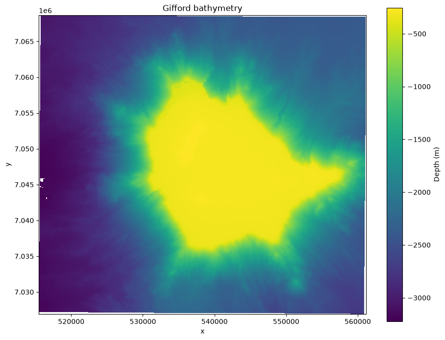

Shaded relief with xarray-spatial¶

A flat color map hides subtle relief. A hillshade simulates illumination from a low sun, which makes ridges and channels pop out. xarray-spatial computes it directly from the DataArray, deriving slope and aspect internally, so we do not write any gradient math. azimuth is the compass direction of the light source and angle_altitude is its height above the horizon.

xarray-spatial follows the GDAL convention and divides the terrain slope by the true cell size, so the shading is computed in real-world units. On the seafloor the horizontal cell size (50 m here) dwarfs the change in depth from one cell to the next, so the real slopes are gentle and a raw hillshade comes out almost flat. The fix is vertical exaggeration: multiply the elevation by a factor before shading, which steepens the apparent slopes and brings the relief back. This is the same idea as LightSource’s vert_exag argument. Larger values give more dramatic relief at the cost of physical accuracy, so treat it as a display choice and tune it by eye.

# scale the depth before shading to bring out the gentle seafloor relief
vert_exag = 5
shaded = hillshade(bathy * vert_exag, azimuth=45, angle_altitude=45)

fig, ax = plt.subplots(figsize=(9, 7), constrained_layout=True)
shaded.plot(ax=ax, cmap="gray", add_colorbar=False)
ax.set_title(f"Gifford hillshade (xarray-spatial, vert_exag={vert_exag})")
ax.set_aspect("equal")
plt.show()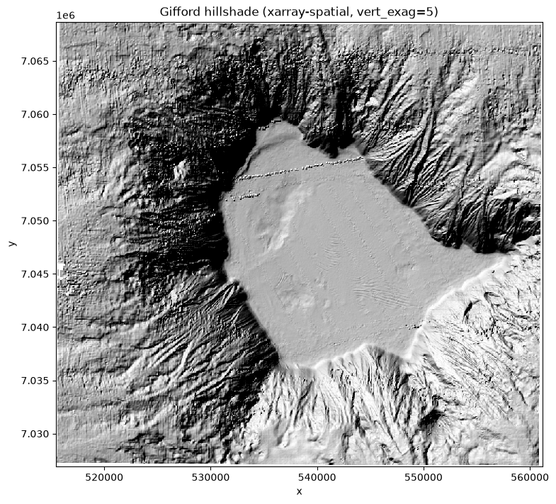

Color-shaded relief by overlaying the hillshade¶

The most readable view combines the depth colormap with the shaded relief. Because the hillshade from the previous cell is itself a labelled DataArray, already vertically exaggerated, we can draw it as a second layer on the same axes: plot the depth in color, then plot the hillshade in grayscale on top with a partial alpha so the colors show through. The dark and light bands of the hillshade then sculpt the flat colormap into relief. Both layers share the same x and y coordinates, so they register exactly with no manual extents.

A lower alpha lets more color through; a higher alpha deepens the shadows.

fig, ax = plt.subplots(figsize=(10, 8), constrained_layout=True)

# base layer: depth in color
bathy.plot(ax=ax, cmap="viridis", cbar_kwargs={"label": "Depth (m)"})

# overlay: the (exaggerated) hillshade from above, grayscale and semi-transparent
shaded.plot(ax=ax, cmap="gray", alpha=0.45, add_colorbar=False)

ax.set_title(f"Gifford color-shaded relief (hillshade overlay, vert_exag={vert_exag})")
ax.set_xlabel("Easting (m)")
ax.set_ylabel("Northing (m)")
ax.xaxis.set_major_formatter(formatter)
ax.yaxis.set_major_formatter(formatter)
ax.set_aspect("equal")
plt.show()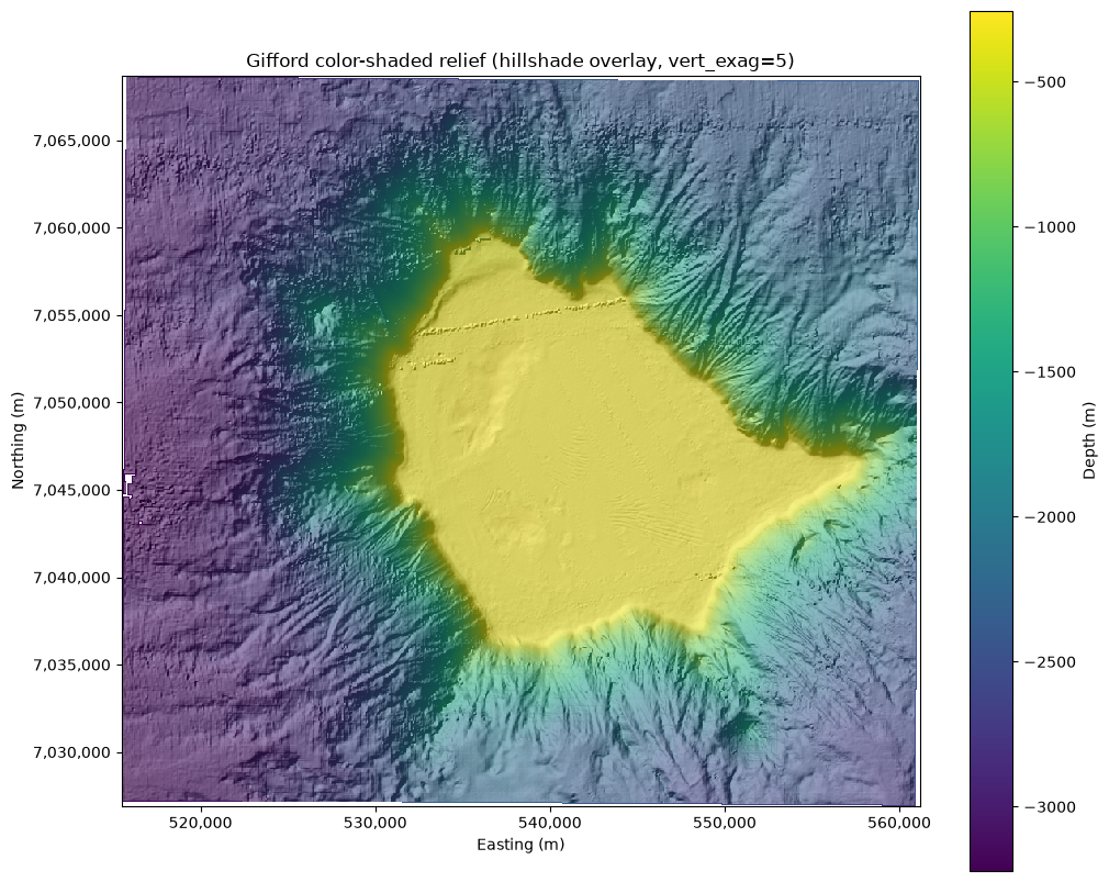

LightSource is another way to do this

We built the color-shaded relief in two explicit steps: compute the hillshade as reusable data with xarray-spatial, then overlay it on the colormap with alpha. Keeping the hillshade as its own DataArray is what makes this possible, and it also lets you save it as a raster or scale the computation across large Dask-backed arrays.

Matplotlib’s matplotlib.colors.LightSource solves the same problem a different way. Its shade method computes a hillshade internally and blends it with a colormap in a single call, returning a ready-made RGB image:

from matplotlib.colors import LightSource

ls = LightSource(azdeg=60, altdeg=45)
rgb = ls.shade(bathy.values, cmap=plt.cm.viridis, vert_exag=50, blend_mode="soft")

The trade-off is that the hillshade stays hidden inside the call, and you manage the map extent and colorbar yourself when drawing the result with imshow. The overlay approach above keeps each layer separate and plots in map coordinates for free.

A reusable function¶

The same three steps, load, shade, and plot, apply to any single-band bathymetry raster. We wrap them in one function, using the hillshade overlay for the relief, and apply it to a second survey, Point Cloates.

def plot_shaded_relief(path, title, azimuth=315, altitude=45,
                       vert_exag=5, alpha=0.45, cmap="viridis"):
    """Load a single-band raster with rioxarray and plot color-shaded relief
    by overlaying a semi-transparent, vertically exaggerated hillshade on the
    depth colormap."""
    da = rioxarray.open_rasterio(path, masked=True).squeeze()
    # exaggerate the vertical relief so the gentle seafloor slopes shade well
    shaded = hillshade(da * vert_exag, azimuth=azimuth, angle_altitude=altitude)

    fig, ax = plt.subplots(figsize=(9, 7), constrained_layout=True)
    da.plot(ax=ax, cmap=cmap, cbar_kwargs={"label": "Depth (m)"})
    shaded.plot(ax=ax, cmap="gray", alpha=alpha, add_colorbar=False)

    ax.set_title(title)
    ax.set_xlabel("Easting (m)")
    ax.set_ylabel("Northing (m)")
    ax.xaxis.set_major_formatter(formatter)
    ax.yaxis.set_major_formatter(formatter)
    ax.set_aspect("equal")
    return da

Applying to another survey¶

pc_bathy = plot_shaded_relief("../data/pc_bathy.tif", "Point Cloates color-shaded relief")
plt.show()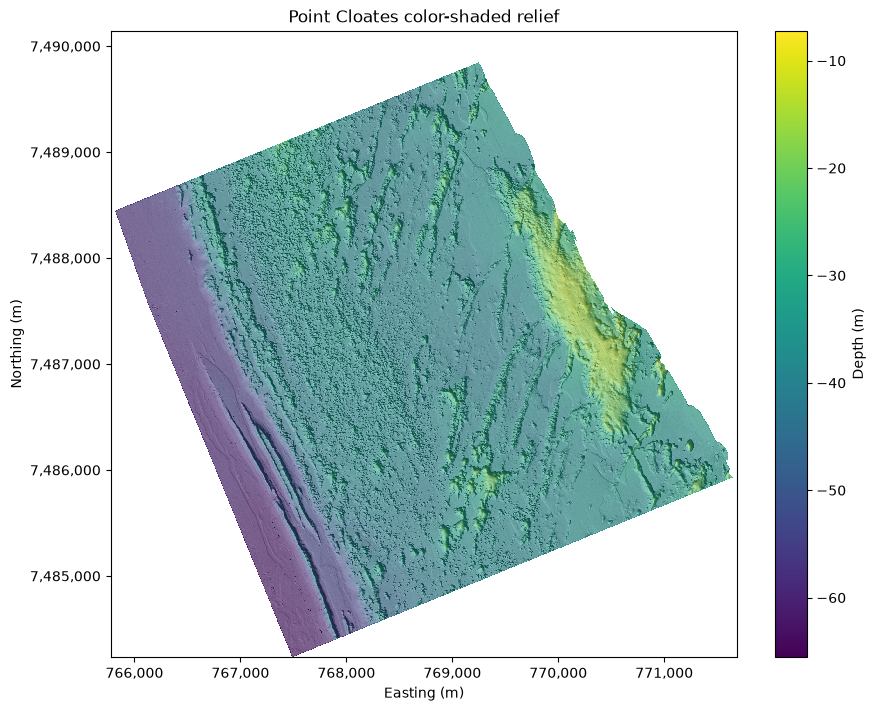

Summary¶

rasterio is the workhorse for reading and writing georeferenced grids. A raster is an array paired with a CRS and an affine transform: the array holds the values, the CRS says where on Earth they sit, and the transform ties pixels to coordinates. You open a file with rasterio.open, inspect its metadata through attributes like crs, res, and transform, and pull band values into NumPy with read, using masked=True to respect nodata. The xy and index methods convert between pixels and map coordinates. For visualization, loading the file with rioxarray gives a labelled, CRS-aware array that plots in map coordinates. xarray-spatial turns it into a hillshade with no hand-written terrain math, and because that hillshade is itself a DataArray we overlay it on the depth colormap with a partial alpha to make color-shaded relief. Matplotlib’s LightSource is an alternative that blends the hillshade into the colormap internally in one call.

What’s next?¶

With raster reading in hand, the following notebooks compute terrain derivatives such as the Topographic Position Index and use them to delineate and classify seabed features.

Resources and References¶

rasterio documentation: https://rasterio.readthedocs.io/
rioxarray documentation: https://corteva.github.io/rioxarray/
xarray-spatial documentation: https://xarray-spatial.readthedocs.io/
Matplotlib LightSource: https://matplotlib.org/stable/api/_as_gen/matplotlib.colors.LightSource.html
Project Pythia Foundations, NumPy and Matplotlib chapters: https://foundations.projectpythia.org/