Discover and Read SAR Data - Earth Observation Data Science Cookbook

This notebook demonstrates how to access radar data in a SpatioTemporal Asset Catalog (STAC) Catalogue using the pystac library. In this example, we use Sentinel-1 data from the EODC (earth observation data and high performance computing service provider based in Vienna) STAC catalog. In the further process, we will learn how to query a STAC catalog, select specific items, and display the metadata and the actual image.

import folium
import pystac_client
from odc import stac as odc_stac

Data Discovery¶

eodc_catalog = pystac_client.Client.open("https://stac.eodc.eu/api/v1")

eodc_catalog

The URL https://stac.eodc.eu/api/v1, served over Hypertext Transfer Protocol (HTTP), is a STAC-compliant API endpoint (specific URL address where an API service is available) that leads to the EODC Catalogue. Besides EODC’s, other catalogues can be found on STAC Index, such as United States Geological Survey (USGS) Landsat imagery, Sentinel Hub, Copernicus Data Space Ecosystem, and so on. Briefly spoken, STAC can be used to search, discover, and access metadata of these datasets with the same code. The EODC Catalogue can be accessed on the web via this link as well.

Each STAC catalog, composed by different providers, has many collections. To get all collections of a catalog, we can print all of them and their ids, which are used to fetch them from the catalog.

collections = eodc_catalog.get_collections()

# length of string of collection.id, for pretty print
max_length = max(len(collection.id) for collection in collections)

for collection in eodc_catalog.get_collections():
    print(f"{collection.id.ljust(max_length)}: {collection.title}")

AI4SAR_SIG0                      : AI4SAR Despeckled Sentinel-1 Sigma0 (20m)
ASA_IMP_1P                       : Envisat ASAR Image Mode Precision Level-1
ASA_IMS_1P                       : Envisat ASAR Image Mode Single Look Complex Level-1
AUSTRIA_GROUND_MOTION            : Austria Ground Motion
AUT_DEM                          : Austrian High Resolution DEM
BOA_LANDSAT_8                    : Bottom of Atmosphere Landsat-8 at 30m resolution.
BOA_SENTINEL_2                   : Bottom of Atmosphere Sentinel-2 at 10m resolution.
CGLS_SSM_1KM                     : Copernicus Global Land Surface Soil Moisture
climatedt                        : DestinE Climate DT - Weather Stations
climatedt-austria                : DestinE Climate Change Adaptation Digital Twin
clms                             : Copernicus Land Monitoring Service
clms-vpp                         : Copernicus Land Monitoring Service - Vegetation Phenology and Productivity
COP_DEM                          : Copernicus Digital Elevation Model (DEM)
CORINE_LAND_COVER                : Corine Land Cover
DOP_AUT_K_KLAGENFURT             : Digital Orthophotos (DOP) Austria - Land Kärnten: Orthofotos Flugblock Klagenfurt
DOP_AUT_K_OSTTIROL               : Digital Orthophotos (DOP) Austria - Land Kärnten: Orthofotos Flugblock Osttirol
DOP_AUT_K_TAMSWEG                : Digital Orthophotos (DOP) Austria - Land Kärnten: Orthofotos Flugblock Tamsweg
DOP_AUT_K_VILLACH                : Digital Orthophotos (DOP) Austria - Land Kärnten: Orthofotos Flugblock Villach
DOP_AUT_K_WOLFSBERG              : Digital Orthophotos (DOP) Austria - Land Kärnten: Orthofotos Flugblock Wolfsberg
DOP_AUT_K_ZELL_AM_SEE            : Digital Orthophotos (DOP) Austria - Land Kärnten: Orthofotos Flugblock Zell am See
DOP_AUT_K_ZELTWEG                : Digital Orthophotos (DOP) Austria - Land Kärnten: Orthofotos Flugblock Zeltweg
DOP_AUT_ST_BISCHOFSHOFEN         : Digital Orthophotos (DOP) Austria - Land Steiermark: Orthophotos Flugblock Bischofshofen
DOP_AUT_ST_GRAZ                  : Digital Orthophotos (DOP) Austria - Land Steiermark: Orthophotos Flugblock Graz
DOP_AUT_ST_KLAGENFURT            : Digital Orthophotos (DOP) Austria - Land Steiermark: Orthophotos Flugblock Klagenfurt
DOP_AUT_ST_MARIAZELL             : Digital Orthophotos (DOP) Austria - Land Steiermark: Orthophotos Flugblock Mariazell
DOP_AUT_ST_MURTAL                : Digital Orthophotos (DOP) Austria - Land Steiermark: Orthophotos Flugblock Murtal
DOP_AUT_ST_SUEDBURGENLAND        : Digital Orthophotos (DOP) Austria - Land Steiermark: Orthophotos Flugblock Suedburgenland
DOP_AUT_ST_VILLACH               : Digital Orthophotos (DOP) Austria - Land Steiermark: Orthophotos Flugblock Villach
DOP_AUT_ST_WINDISCHGARSTEN       : Digital Orthophotos (DOP) Austria - Land Steiermark: Orthophotos Flugblock Windischgarsten
DROUGHT_VULNERABILITY            : Drought Vulnerability
DSM_AUT                          : Austrian Digital Surface Model
ERS_ENVISAT_NRB                  : ERS-1/2 SAR and ENVISAT ASAR ARD Normalized Radar Backscatter (NRB)
GFM                              : Global Flood Monitoring
incal-hourly                     : INCA analysis hourly data (1km)
INTRA_FIELD_CROP_GROWTH_POTENTIAL: Intra-field Crop Growth Potential
RUCIO_SENTINEL2_MFCOVER          : Monthly Composite of Fraction of Vegetation Cover
SAR_IMP_1P                       : ERS-1/2 SAR Image Mode Precision Level-1
SAR_IMS_1P                       : ERS-1/2 SAR Image Mode Single Look Complex Level-1
SENTINEL1_ALPS_WETSNOW           : Sentinel-1 Alps WetSnow
SENTINEL1_GMR0                   : SENTINEL1 Radiometric Terrain Corrected Gamma Nought
SENTINEL1_GRD                    : Sentinel-1 SAR L1 GRD
SENTINEL1_GRD_COVERAGE           : Sentinel-1 Coverage Maps
SENTINEL1_HPAR                   : SENTINEL1 Harmonic Parameters
Sentinel-1_Lacken_Extent         : SENTINEL-1 Lacken Extent
SENTINEL1_MPLIA                  : SENTINEL1 Mean PLIA
Sentinel-1_Reed_Extent           : SENTINEL-1 Reed Extent
SENTINEL1_SCENE_GMR0             : SENTINEL1 Scene-based Radiometric Terrain Corrected Gamma Nought
SENTINEL1_SIG0_20M               : SENTINEL1 Sigma Nought (SIG0) Backscatter in 20 meter resolution
SENTINEL1_SLC                    : Sentinel-1 SLC
Sentinel-2-Greenness-Austria     : Sentinel-2 Greenness Austria
SENTINEL2_GRI_L1C                : Multi-Layer Copernicus Sentinel-2 GRI in L1C
SENTINEL2_L1C                    : Sentinel-2 MSI Products: Level-1C data
SENTINEL2_L1C_COVERAGE           : Sentinel-2 L1C Coverage Maps
SENTINEL2_L2A                    : Sentinel-2 MSI Products: Level-2A data
sentinel2-landsat8-l2f           : Harmonized Landsat and Sentinel 2 L2F
SENTINEL2_MFCOVER                : Monthly Composite of Fraction of Vegetation Cover
SENTINEL3_SRAL_L2                : Sentinel-3 Products: SRAL Level-2 data
SENTINEL5P_DAILY_AUT             : Sentinel-5P Daily Aggregated Atmospheric Data for Austria
spartacus-daily                  : Spartacus Analysis Daily (1 km)
SSM-RT0-SIG0-R-EXTR              : SSM-RT0-SIG0-R-EXTR
topo-dc-austria-dsm              : Digital surface model (1m x 1m) [TOPO4EO]
topo-dc-austria-dtm              : Digital terrain model (1m x 1m) [TOPO4EO]
topo-dc-austria-ndsm             : Normalized digital surface model (1m x 1m) [TOPO4EO]
VEGETATION_CHANGE_AUSTRIA        : Vegetation-Change-Austria

To get a specific collection from the catalog, we can use the client.get_collection() method and provide the collection name. We can then display its description, id, temporal and spatial extent, license, etc. In this notebook, we will work with the Sentinel-1 sigma naught 20m collection.

colllection_id = "SENTINEL1_SIG0_20M"

collection = eodc_catalog.get_collection(colllection_id)
collection

Each collection has multiple items. An item is one spatio-temporal instance in the collection, for instance a satellite image. If items are needed for a specific timeframe or for a specific region of interest, we can define this as a query.

time_range = "2022-10-01/2022-10-07"  # a closed range
# time_range = "2022-01"  # whole month, same can be done for a year and a day
# time_range = "2022-01-01/.."  # up to the current date, an open range
# time_range = "2022-01-01T05:34:46"  # a specific time instance

A spatial region of interest can be defined in different ways. One option is to define a simple bounding box:

latmin, latmax = 46.3, 49.3  # South to North
lonmin, lonmax = 13.8, 17.8  # West to East

bounding_box = [lonmin, latmin, lonmax, latmax]

If the region of interest is not rectangular, we can also define a polygon:

# GEOJSON can be created on geojson.io

# This specific area of interest is a rectangle, but since it is
# a closed polygon it seems like it has five nodes

area_of_interest = {
    "coordinates": [
        [
            [17.710928010825853, 49.257630084442496],
            [13.881798300915221, 49.257630084442496],
            [13.881798300915221, 46.34747715326259],
            [17.710928010825853, 46.34747715326259],
            [17.710928010825853, 49.257630084442496],
        ]
    ],
    "type": "Polygon",
}

Using our previously loaded STAC catalog, we can now search for items fullfilling our query. In this example we are using the bounding box. If we want to use an area of interest specified in the geojson format - one has to use the intersects parameter as documented in the comment below.

search = eodc_catalog.search(
    collections=colllection_id,  # can also be a list of several collections
    bbox=bounding_box,  # search by bounding box
    # intersects=area_of_interest,  # GeoJSON search
    datetime=time_range,
    # max_items=1  # number of max items to load
)

# If we comment everything besides colllection_id, we will load whole
# collection for available region and time_range

items_eodc = search.item_collection()
print(f"On EODC we found {len(items_eodc)} items for the given search query")

On EODC we found 52 items for the given search query

Now, we can fetch a single item, in this case a Sentinel-1 image, from the query results. A good practice is to always check what metadata the data provider has stored on the item level. This can be done by looking into the item properties.

item = items_eodc[0]
item.properties

{'gsd': 20,
 'parent': 'S1A_IW_GRDH_1SDV_20221007T170811_20221007T170836_045339_056BBA_D830.zip',
 'checksum': '576abe68a715e5ee177d8b640871e873',
 'datetime': '2022-10-07T17:08:11Z',
 'blocksize': {'x': 15000, 'y': 5},
 'proj:bbox': [4800000, 1500000, 5100000, 1800000],
 'proj:wkt2': 'PROJCS["Azimuthal_Equidistant",GEOGCS["WGS 84",DATUM["WGS_1984",SPHEROID["WGS 84",6378137,298.257223563,AUTHORITY["EPSG","7030"]],AUTHORITY["EPSG","6326"]],PRIMEM["Greenwich",0],UNIT["degree",0.0174532925199433],AUTHORITY["EPSG","4326"]],PROJECTION["Azimuthal_Equidistant"],PARAMETER["latitude_of_center",53],PARAMETER["longitude_of_center",24],PARAMETER["false_easting",5837287.81977],PARAMETER["false_northing",2121415.69617],UNIT["metre",1,AUTHORITY["EPSG","9001"]]]',
 'proj:shape': [15000, 15000],
 'Equi7_TileID': 'EU020M_E048N015T3',
 'constellation': 'sentinel-1',
 'proj:geometry': {'type': 'Polygon',
  'coordinates': [[[4800000.0, 1500000.0],
    [4800000.0, 1800000.0],
    [5100000.0, 1800000.0],
    [5100000.0, 1500000.0],
    [4800000.0, 1500000.0]]]},
 'proj:transform': [20, 0, 4800000, 0, -20, 1800000],
 'sat:orbit_state': 'ascending',
 'sar:product_type': 'GRD',
 'slice_gap_filled': False,
 'sar:polarizations': ['VH', 'VV'],
 'sar:frequency_band': 'C',
 'sat:relative_orbit': 117,
 'sar:instrument_mode': 'IW',
 'border_noise_removed': True,
 'sar:center_frequency': 5.405,
 'sar:resolution_range': 40,
 'thermal_noise_removed': True,
 'sar:resolution_azimuth': 40,
 'sar:pixel_spacing_range': 20,
 'sar:observation_direction': 'right',
 'sar:pixel_spacing_azimuth': 20,
 'sat:platform_international_designator': '2014-016A'}

For now, let’s display only the vertical-vertical (VV) polarized band of the item and some information about the data.

item.assets["VV"].extra_fields.get("raster:bands")[0]

{'scale': 10,
 'nodata': -9999,
 'offset': 0,
 'data_type': 'int16',
 'spatial_resolution': 20}

In the EODC STAC catalogue an item can conveniently be displayed using its thumbnail.

item.assets["thumbnail"].href

'https://data.eodc.eu/collections/SENTINEL1_SIG0_20M/V1M1R1/EQUI7_EU020M/E048N015T3/SIG0_20221007T170811__VV_A117_E048N015T3_EU020M_V1M1R1_S1AIWGRDH_TUWIEN.tif/thumbnail'

Now we will plot the data on a map using the thumbnail and the python package folium. This is an easy way to quickly check how the data found by a search query looks on a map.

map = folium.Map(
    location=[(latmin + latmax) / 2, (lonmin + lonmax) / 2],
    zoom_start=7,
    zoom_control=False,
    scrollWheelZoom=False,
    dragging=False,
)

folium.GeoJson(area_of_interest, name="Area of Interest").add_to(map)

for item in items_eodc:
    # url leading to display of an item, can also be used as hyperlink
    image_url = item.assets["thumbnail"].href
    bounds = item.bbox
    folium.raster_layers.ImageOverlay(
        image=image_url,
        bounds=[[bounds[1], bounds[0]], [bounds[3], bounds[2]]],
    ).add_to(map)

folium.LayerControl().add_to(map)

map

Figure 1: Map of study area. Blue rectangle is the area covered by the discovered data.

Data Reading¶

STAC can also be a useful tool for the discovery of data, however it only loads metadata. This saves memory, but if one would like to do further analysis, the data has to be loaded into memory or downloaded on disk.

In the following, we will demonstrate this with the library odc-stac. Here we can define what data will loaded as bands; in this case VV sigma naught. Moreover we can resample the data by providing any coordinate reference system (CRS) and resolution as well as a method for resampling of continuos data (e.g. bilinear resampling). In the example below we use the EQUI7 Grid of Europe and a 20 meter sampling. This is the native format of sigma naught stored at EODC, so there will be no actual resampling. Note, also, that resampling is not advisable for this data, as it is provided on a logarithmic scale. More about this in the notebook “Backscattering Coefficients”.

The chunks argument is an advancement method for performing parallel computations on the data. We will not cover this in further detail.

bands = "VV"  # Vertical-vertical polarized
crs = "EPSG:27704"  # Coordinate Reference System: EQUI7 Grid of Europe
res = 20  # 20 meter
chunks = {"time": 1, "latitude": 1000, "longitude": 1000}
sig0_dc = odc_stac.load(
    items_eodc,
    bands=bands,
    crs=crs,
    resolution=res,
    bbox=bounding_box,
    chunks=chunks,
    resampling="bilinear",
)

Let’s have a look at the VV polarized band of the dataset.

sig0_dc.VV

As we can see, the data is stored as a xarray DataArray. Xarray is a convenient package for multidimensional labeled arrays, like temperature, humidity, pressure, different bands of satellite imagery, and so on. The link provides detailed documentation. In a later notebook we will explore some more of the functionality of xarray. As we can see in the coordinates, the data here consists of 21 time steps.

In general, data from STAC is “lazily” loaded, which means that the structure of the DataArray is constructed, but the data is not loaded yet. It is loaded only at instance when it is needed, for example, for plotting, computations, and so on.

Since the DataArray has currently a size of almost 18 GiB, we will subset it to the region of Vienna.

# Create a bounding box covering the region of Vienna
latmin_smaller, latmax_smaller = 48, 48.4
lonmin_smaller, lonmax_smaller = 16, 16.5

smaller_bounding_box = [
    [latmin_smaller, lonmin_smaller],
    [latmax_smaller, lonmax_smaller],
]

map = folium.Map(
    location=[
        (latmin_smaller + latmax_smaller) / 2,
        (lonmin_smaller + lonmax_smaller) / 2,
    ],
    zoom_start=8,
    zoom_control=False,
    scrollWheelZoom=False,
    dragging=False,
)

folium.GeoJson(area_of_interest, name="Area of Interest").add_to(map)

folium.Rectangle(
    bounds=smaller_bounding_box,
    color="red",
).add_to(map)

for item in items_eodc:
    image_url = item.assets["thumbnail"].href
    bounds = item.bbox
    folium.raster_layers.ImageOverlay(
        image=image_url,
        bounds=[[bounds[1], bounds[0]], [bounds[3], bounds[2]]],
    ).add_to(map)

folium.LayerControl().add_to(map)

map

Figure 2: Map of study area. Blue rectangle is the area covered by the discovered data. Red rectangle covers the selected data.

Create a new dataset with the smaller bounding box covering the region of Vienna. We will leave out the arguments for resampling and directly use the native format as defined in the metadata.

sig0_dc = odc_stac.load(
    items_eodc,
    bands=bands,
    bbox=[lonmin_smaller, latmin_smaller, lonmax_smaller, latmax_smaller],
    chunks=chunks,
)

Due to the way the data is acquired and stored, some items include “no data” areas. In our case, no data has the value -9999, but this can vary from data provider to data provider. This information can usually be found in the metadata. Furthermore, to save memory, data is often stored as integer (e.g. 25) and not in float (e.g. 2.5) format. For this reason, the backscatter values are often multiplied by a scale factor, in this case factor 10.

As Sentinel-1 satellites overpasses Austria every few days, only some time steps of the dataset will have physical data. As a final step, we will now decode the data and create a plot of two consecutive Sentinel-1 acquisitions of Vienna.

# Retrieve the scale factor and NoData value from the metadata. raster:bands is
# a STAC raster extension
scale = item.assets["VV"].extra_fields.get("raster:bands")[0]["scale"]
nodata = item.assets["VV"].extra_fields.get("raster:bands")[0]["nodata"]

# Decode data with the NoData value and the scale factor
sig0_dc = sig0_dc.where(sig0_dc != nodata) / scale

# We should remove unnecessary dates when there was no data
# (no satellite overpass)
sig0_dc = sig0_dc.dropna(dim="time")

sig0_dc.VV.plot(col="time", robust=True, cmap="Greys_r", aspect=1, size=10)

---------------------------------------------------------------------------
ValueError                                Traceback (most recent call last)
Cell In[18], line 1
----> 1 sig0_dc.VV.plot(col="time", robust=True, cmap="Greys_r", aspect=1, size=10)

File ~/micromamba/envs/eo-datascience-cookbook/lib/python3.13/site-packages/xarray/plot/accessor.py:48, in DataArrayPlotAccessor.__call__(self, **kwargs)
     46 @functools.wraps(dataarray_plot.plot, assigned=("__doc__", "__annotations__"))
     47 def __call__(self, **kwargs) -> Any:
---> 48     return dataarray_plot.plot(self._da, **kwargs)

File ~/micromamba/envs/eo-datascience-cookbook/lib/python3.13/site-packages/xarray/plot/dataarray_plot.py:318, in plot(darray, row, col, col_wrap, ax, hue, subplot_kws, **kwargs)
    314     plotfunc = hist
    316 kwargs["ax"] = ax
--> 318 return plotfunc(darray, **kwargs)

File ~/micromamba/envs/eo-datascience-cookbook/lib/python3.13/site-packages/xarray/plot/dataarray_plot.py:1518, in _plot2d.<locals>.newplotfunc(***failed resolving arguments***)
   1516     # Need the decorated plotting function
   1517     allargs["plotfunc"] = globals()[plotfunc.__name__]
-> 1518     return _easy_facetgrid(darray, kind="dataarray", **allargs)
   1520 if darray.ndim == 0 or darray.size == 0:
   1521     # TypeError to be consistent with pandas
   1522     raise TypeError("No numeric data to plot.")

File ~/micromamba/envs/eo-datascience-cookbook/lib/python3.13/site-packages/xarray/plot/facetgrid.py:1117, in _easy_facetgrid(data, plotfunc, kind, x, y, row, col, col_wrap, sharex, sharey, aspect, size, subplot_kws, ax, figsize, **kwargs)
   1114     return g.map_dataarray_line(plotfunc, x, y, **kwargs)
   1116 if kind == "dataarray":
-> 1117     return g.map_dataarray(plotfunc, x, y, **kwargs)
   1119 if kind == "plot1d":
   1120     return g.map_plot1d(plotfunc, x, y, **kwargs)

File ~/micromamba/envs/eo-datascience-cookbook/lib/python3.13/site-packages/xarray/plot/facetgrid.py:426, in FacetGrid.map_dataarray(self, func, x, y, **kwargs)
    423 self._finalize_grid(xlabel, ylabel)
    425 if kwargs.get("add_colorbar", True):
--> 426     self.add_colorbar(**cbar_kwargs)
    428 return self

File ~/micromamba/envs/eo-datascience-cookbook/lib/python3.13/site-packages/xarray/plot/facetgrid.py:793, in FacetGrid.add_colorbar(self, **kwargs)
    791     assert isinstance(self.data, DataArray)
    792     kwargs.setdefault("label", label_from_attrs(self.data))
--> 793 self.cbar = self.fig.colorbar(
    794     self._mappables[-1], ax=list(self.axs.flat), **kwargs
    795 )

File ~/micromamba/envs/eo-datascience-cookbook/lib/python3.13/site-packages/matplotlib/figure.py:1300, in FigureBase.colorbar(self, mappable, cax, ax, use_gridspec, **kwargs)
   1298     cax, kwargs = cbar.make_axes_gridspec(ax, **kwargs)
   1299 else:
-> 1300     cax, kwargs = cbar.make_axes(ax, **kwargs)
   1301 # make_axes calls add_{axes,subplot} which changes gca; undo that.
   1302 fig.sca(current_ax)

File ~/micromamba/envs/eo-datascience-cookbook/lib/python3.13/site-packages/matplotlib/colorbar.py:1476, in make_axes(parents, location, orientation, fraction, shrink, aspect, **kwargs)
   1473     if panchor is not False:
   1474         ax.set_anchor(panchor)
-> 1476 cax = fig.add_axes(pbcb, label="<colorbar>")
   1477 for a in parents:
   1478     a._colorbars.append(cax)  # tell the parent it has a colorbar

File ~/micromamba/envs/eo-datascience-cookbook/lib/python3.13/site-packages/matplotlib/figure.py:642, in FigureBase.add_axes(self, *args, **kwargs)
    640 rect, = args
    641 if not np.isfinite(rect).all():
--> 642     raise ValueError(f'all entries in rect must be finite not {rect}')
    643 projection_class, pkw = self._process_projection_requirements(**kwargs)
    645 # create the new Axes using the Axes class given

ValueError: all entries in rect must be finite not Bbox(x0=nan, y0=nan, x1=nan, y1=nan)

Error in callback <function _draw_all_if_interactive at 0x7f5f641234c0> (for post_execute), with arguments args (),kwargs {}:

---------------------------------------------------------------------------
ValueError                                Traceback (most recent call last)
File ~/micromamba/envs/eo-datascience-cookbook/lib/python3.13/site-packages/matplotlib/pyplot.py:300, in _draw_all_if_interactive()
    298 def _draw_all_if_interactive() -> None:
    299     if matplotlib.is_interactive():
--> 300         draw_all()

File ~/micromamba/envs/eo-datascience-cookbook/lib/python3.13/site-packages/matplotlib/_pylab_helpers.py:133, in Gcf.draw_all(cls, force)
    131 for manager in cls.get_all_fig_managers():
    132     if force or manager.canvas.figure.stale:
--> 133         manager.canvas.draw_idle()

File ~/micromamba/envs/eo-datascience-cookbook/lib/python3.13/site-packages/matplotlib/backend_bases.py:1989, in FigureCanvasBase.draw_idle(self, *args, **kwargs)
   1987 if not self._is_idle_drawing:
   1988     with self._idle_draw_cntx():
-> 1989         self.draw(*args, **kwargs)

File ~/micromamba/envs/eo-datascience-cookbook/lib/python3.13/site-packages/matplotlib/backends/backend_agg.py:438, in FigureCanvasAgg.draw(self)
    435 # Acquire a lock on the shared font cache.
    436 with (self.toolbar._wait_cursor_for_draw_cm() if self.toolbar
    437       else nullcontext()):
--> 438     self.figure.draw(self.renderer)
    439     # A GUI class may be need to update a window using this draw, so
    440     # don't forget to call the superclass.
    441     super().draw()

File ~/micromamba/envs/eo-datascience-cookbook/lib/python3.13/site-packages/matplotlib/artist.py:94, in _finalize_rasterization.<locals>.draw_wrapper(artist, renderer, *args, **kwargs)
     92 @wraps(draw)
     93 def draw_wrapper(artist, renderer, *args, **kwargs):
---> 94     result = draw(artist, renderer, *args, **kwargs)
     95     if renderer._rasterizing:
     96         renderer.stop_rasterizing()

File ~/micromamba/envs/eo-datascience-cookbook/lib/python3.13/site-packages/matplotlib/artist.py:71, in allow_rasterization.<locals>.draw_wrapper(artist, renderer)
     68     if artist.get_agg_filter() is not None:
     69         renderer.start_filter()
---> 71     return draw(artist, renderer)
     72 finally:
     73     if artist.get_agg_filter() is not None:

File ~/micromamba/envs/eo-datascience-cookbook/lib/python3.13/site-packages/matplotlib/figure.py:3282, in Figure.draw(self, renderer)
   3279             # ValueError can occur when resizing a window.
   3281     self.patch.draw(renderer)
-> 3282     mimage._draw_list_compositing_images(
   3283         renderer, self, artists, self.suppressComposite)
   3285     renderer.close_group('figure')
   3286 finally:

File ~/micromamba/envs/eo-datascience-cookbook/lib/python3.13/site-packages/matplotlib/image.py:133, in _draw_list_compositing_images(renderer, parent, artists, suppress_composite)
    131 if not_composite or not has_images:
    132     for a in artists:
--> 133         a.draw(renderer)
    134 else:
    135     # Composite any adjacent images together
    136     image_group = []

File ~/micromamba/envs/eo-datascience-cookbook/lib/python3.13/site-packages/matplotlib/artist.py:71, in allow_rasterization.<locals>.draw_wrapper(artist, renderer)
     68     if artist.get_agg_filter() is not None:
     69         renderer.start_filter()
---> 71     return draw(artist, renderer)
     72 finally:
     73     if artist.get_agg_filter() is not None:

File ~/micromamba/envs/eo-datascience-cookbook/lib/python3.13/site-packages/matplotlib/axes/_base.py:3314, in _AxesBase.draw(self, renderer)
   3311     for spine in self.spines.values():
   3312         artists.remove(spine)
-> 3314 self._update_title_position(renderer)
   3316 if not self.axison:
   3317     for _axis in self._axis_map.values():

File ~/micromamba/envs/eo-datascience-cookbook/lib/python3.13/site-packages/matplotlib/axes/_base.py:3258, in _AxesBase._update_title_position(self, renderer)
   3256 if title.get_text():
   3257     for ax in axs:
-> 3258         ax.yaxis.get_tightbbox(renderer)  # update offsetText
   3259         if ax.yaxis.offsetText.get_text():
   3260             bb = ax.yaxis.offsetText.get_tightbbox(renderer)

File ~/micromamba/envs/eo-datascience-cookbook/lib/python3.13/site-packages/matplotlib/axis.py:1425, in Axis.get_tightbbox(self, renderer, for_layout_only)
   1423 if renderer is None:
   1424     renderer = self.get_figure(root=True)._get_renderer()
-> 1425 ticks_to_draw = self._update_ticks()
   1427 self._update_label_position(renderer)
   1429 # go back to just this axis's tick labels

File ~/micromamba/envs/eo-datascience-cookbook/lib/python3.13/site-packages/matplotlib/axis.py:1344, in Axis._update_ticks(self)
   1340 # Check if major ticks should be computed.
   1341 # Skip if using NullLocator or if all visible components are off.
   1342 if (self._tick_group_visible(self._major_tick_kw)
   1343         and not isinstance(self.get_major_locator(), NullLocator)):
-> 1344     major_locs = self.get_majorticklocs()
   1345     major_labels = self.major.formatter.format_ticks(major_locs)
   1346     major_ticks = self.get_major_ticks(len(major_locs))

File ~/micromamba/envs/eo-datascience-cookbook/lib/python3.13/site-packages/matplotlib/axis.py:1673, in Axis.get_majorticklocs(self)
   1671 def get_majorticklocs(self):
   1672     """Return this Axis' major tick locations in data coordinates."""
-> 1673     return self.major.locator()

File ~/micromamba/envs/eo-datascience-cookbook/lib/python3.13/site-packages/matplotlib/ticker.py:2299, in MaxNLocator.__call__(self)
   2297 def __call__(self):
   2298     vmin, vmax = self.axis.get_view_interval()
-> 2299     return self.tick_values(vmin, vmax)

File ~/micromamba/envs/eo-datascience-cookbook/lib/python3.13/site-packages/matplotlib/ticker.py:2307, in MaxNLocator.tick_values(self, vmin, vmax)
   2304     vmin = -vmax
   2305 vmin, vmax = mtransforms._nonsingular(
   2306     vmin, vmax, expander=1e-13, tiny=1e-14)
-> 2307 locs = self._raw_ticks(vmin, vmax)
   2309 prune = self._prune
   2310 if prune == 'lower':

File ~/micromamba/envs/eo-datascience-cookbook/lib/python3.13/site-packages/matplotlib/ticker.py:2237, in MaxNLocator._raw_ticks(self, vmin, vmax)
   2235 if self._nbins == 'auto':
   2236     if self.axis is not None:
-> 2237         nbins = np.clip(self.axis.get_tick_space(),
   2238                         max(1, self._min_n_ticks - 1), 9)
   2239     else:
   2240         nbins = 9

File ~/micromamba/envs/eo-datascience-cookbook/lib/python3.13/site-packages/matplotlib/axis.py:2984, in YAxis.get_tick_space(self)
   2982 size = self._get_tick_label_size('y') * 2
   2983 if size > 0:
-> 2984     return int(np.floor(length / size))
   2985 else:
   2986     return 2**31 - 1

ValueError: cannot convert float NaN to integer

---------------------------------------------------------------------------
ValueError                                Traceback (most recent call last)
File ~/micromamba/envs/eo-datascience-cookbook/lib/python3.13/site-packages/matplotlib/backend_bases.py:2249, in FigureCanvasBase.print_figure(self, filename, dpi, facecolor, edgecolor, orientation, format, bbox_inches, pad_inches, bbox_extra_artists, backend, **kwargs)
   2246     # we do this instead of `self.figure.draw_without_rendering`
   2247     # so that we can inject the orientation
   2248     with getattr(renderer, "_draw_disabled", nullcontext)():
-> 2249         self.figure.draw(renderer)
   2250 else:
   2251     renderer = None

File ~/micromamba/envs/eo-datascience-cookbook/lib/python3.13/site-packages/matplotlib/artist.py:94, in _finalize_rasterization.<locals>.draw_wrapper(artist, renderer, *args, **kwargs)
     92 @wraps(draw)
     93 def draw_wrapper(artist, renderer, *args, **kwargs):
---> 94     result = draw(artist, renderer, *args, **kwargs)
     95     if renderer._rasterizing:
     96         renderer.stop_rasterizing()

File ~/micromamba/envs/eo-datascience-cookbook/lib/python3.13/site-packages/matplotlib/artist.py:71, in allow_rasterization.<locals>.draw_wrapper(artist, renderer)
     68     if artist.get_agg_filter() is not None:
     69         renderer.start_filter()
---> 71     return draw(artist, renderer)
     72 finally:
     73     if artist.get_agg_filter() is not None:

File ~/micromamba/envs/eo-datascience-cookbook/lib/python3.13/site-packages/matplotlib/figure.py:3282, in Figure.draw(self, renderer)
   3279             # ValueError can occur when resizing a window.
   3281     self.patch.draw(renderer)
-> 3282     mimage._draw_list_compositing_images(
   3283         renderer, self, artists, self.suppressComposite)
   3285     renderer.close_group('figure')
   3286 finally:

File ~/micromamba/envs/eo-datascience-cookbook/lib/python3.13/site-packages/matplotlib/image.py:133, in _draw_list_compositing_images(renderer, parent, artists, suppress_composite)
    131 if not_composite or not has_images:
    132     for a in artists:
--> 133         a.draw(renderer)
    134 else:
    135     # Composite any adjacent images together
    136     image_group = []

File ~/micromamba/envs/eo-datascience-cookbook/lib/python3.13/site-packages/matplotlib/artist.py:71, in allow_rasterization.<locals>.draw_wrapper(artist, renderer)
     68     if artist.get_agg_filter() is not None:
     69         renderer.start_filter()
---> 71     return draw(artist, renderer)
     72 finally:
     73     if artist.get_agg_filter() is not None:

File ~/micromamba/envs/eo-datascience-cookbook/lib/python3.13/site-packages/matplotlib/axes/_base.py:3314, in _AxesBase.draw(self, renderer)
   3311     for spine in self.spines.values():
   3312         artists.remove(spine)
-> 3314 self._update_title_position(renderer)
   3316 if not self.axison:
   3317     for _axis in self._axis_map.values():

File ~/micromamba/envs/eo-datascience-cookbook/lib/python3.13/site-packages/matplotlib/axes/_base.py:3258, in _AxesBase._update_title_position(self, renderer)
   3256 if title.get_text():
   3257     for ax in axs:
-> 3258         ax.yaxis.get_tightbbox(renderer)  # update offsetText
   3259         if ax.yaxis.offsetText.get_text():
   3260             bb = ax.yaxis.offsetText.get_tightbbox(renderer)

File ~/micromamba/envs/eo-datascience-cookbook/lib/python3.13/site-packages/matplotlib/axis.py:1425, in Axis.get_tightbbox(self, renderer, for_layout_only)
   1423 if renderer is None:
   1424     renderer = self.get_figure(root=True)._get_renderer()
-> 1425 ticks_to_draw = self._update_ticks()
   1427 self._update_label_position(renderer)
   1429 # go back to just this axis's tick labels

File ~/micromamba/envs/eo-datascience-cookbook/lib/python3.13/site-packages/matplotlib/axis.py:1344, in Axis._update_ticks(self)
   1340 # Check if major ticks should be computed.
   1341 # Skip if using NullLocator or if all visible components are off.
   1342 if (self._tick_group_visible(self._major_tick_kw)
   1343         and not isinstance(self.get_major_locator(), NullLocator)):
-> 1344     major_locs = self.get_majorticklocs()
   1345     major_labels = self.major.formatter.format_ticks(major_locs)
   1346     major_ticks = self.get_major_ticks(len(major_locs))

File ~/micromamba/envs/eo-datascience-cookbook/lib/python3.13/site-packages/matplotlib/axis.py:1673, in Axis.get_majorticklocs(self)
   1671 def get_majorticklocs(self):
   1672     """Return this Axis' major tick locations in data coordinates."""
-> 1673     return self.major.locator()

File ~/micromamba/envs/eo-datascience-cookbook/lib/python3.13/site-packages/matplotlib/ticker.py:2299, in MaxNLocator.__call__(self)
   2297 def __call__(self):
   2298     vmin, vmax = self.axis.get_view_interval()
-> 2299     return self.tick_values(vmin, vmax)

File ~/micromamba/envs/eo-datascience-cookbook/lib/python3.13/site-packages/matplotlib/ticker.py:2307, in MaxNLocator.tick_values(self, vmin, vmax)
   2304     vmin = -vmax
   2305 vmin, vmax = mtransforms._nonsingular(
   2306     vmin, vmax, expander=1e-13, tiny=1e-14)
-> 2307 locs = self._raw_ticks(vmin, vmax)
   2309 prune = self._prune
   2310 if prune == 'lower':

File ~/micromamba/envs/eo-datascience-cookbook/lib/python3.13/site-packages/matplotlib/ticker.py:2237, in MaxNLocator._raw_ticks(self, vmin, vmax)
   2235 if self._nbins == 'auto':
   2236     if self.axis is not None:
-> 2237         nbins = np.clip(self.axis.get_tick_space(),
   2238                         max(1, self._min_n_ticks - 1), 9)
   2239     else:
   2240         nbins = 9

File ~/micromamba/envs/eo-datascience-cookbook/lib/python3.13/site-packages/matplotlib/axis.py:2984, in YAxis.get_tick_space(self)
   2982 size = self._get_tick_label_size('y') * 2
   2983 if size > 0:
-> 2984     return int(np.floor(length / size))
   2985 else:
   2986     return 2**31 - 1

ValueError: cannot convert float NaN to integer

<Figure size 2100x1000 with 2 Axes>

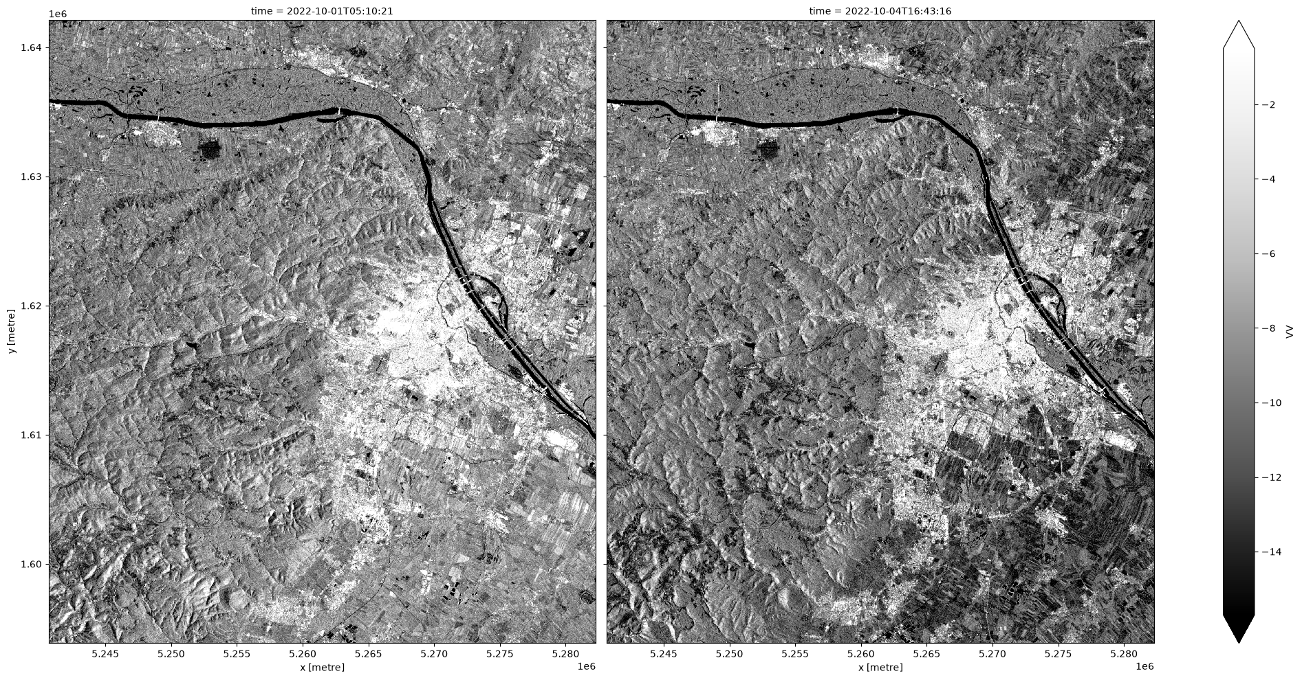
Figure 3: Sentinel-1 microwave backscatter image for two timeslices.