Interferograms

On July 5th, 2019, an earthquake with a magnitude of 7.1 mainshock struck eastern California, near the city of Ridgecrest. The seismic event produced a surface rupture spanning more than 50 kilometers with a complex vertical and horizontal offset pattern along the main fault line. SAR imagery can be employed for accurately measuring and describing ground motion through a well-established technique called SAR Interferometry. In this framework, the phase information contained in Synthetic Aperture Radar (SAR) data is employed. In this notebook, we will dive into the main interferometric SAR processing operations which involves retrieving the difference between the phase signals of repeated SAR acquisitions to analyze the shape and deformation of the Earth’s surface. In our case, we will use a pair of Single Look Complex (SLC) Sentinel-1 images to obtain an interferogram of the Ridgecrest earthquake.

This notebook will outline the process of working with interferograms and the steps needed to extract valuable information. Here, we will focus on displaying products generated by the Sentinel Application Platform (SNAP) software from the European Space Agency (ESA).

Photo by Brian Olson / California Geological Survey

import base64
from io import BytesIO

import folium
import holoviews as hv
import hvplot.xarray  # noqa: F401
import intake
import matplotlib.pyplot as plt
import seaborn as sns

hv.extension("bokeh")

Single Look Complex (SLC) Data

We introduce now another level-1 radar product type, which is called Single Look Complex (SLC). Interferometry can only be performed with SLC data. What are the main differences between SLC and GRD (the other level-1 radar product)?

• SLC vs GRD:

  • SLC contains complex-value data (amplitude and phase) vs GRD contains intensity only (amplitude)

  • SLC geometry is Slant Range (radar’s line of sight) vs GRD data are projected onto ground range

  • SLC resolution is full vs GRD has lower resolution (it is multi-looked)

  • SLC supports phase-based applications (Interferometry) vs GRD supports only amplitude-based ones

  • SLC has larger file sizes compared to GRD

uri = "https://git.geo.tuwien.ac.at/public_projects/microwave-remote-sensing/-/raw/main/microwave-remote-sensing.yml"
cat = intake.open_catalog(uri)
iw1_ds = cat.iw1.read()
iw2_ds = cat.iw2.read()
iw3_ds = cat.iw3.read()

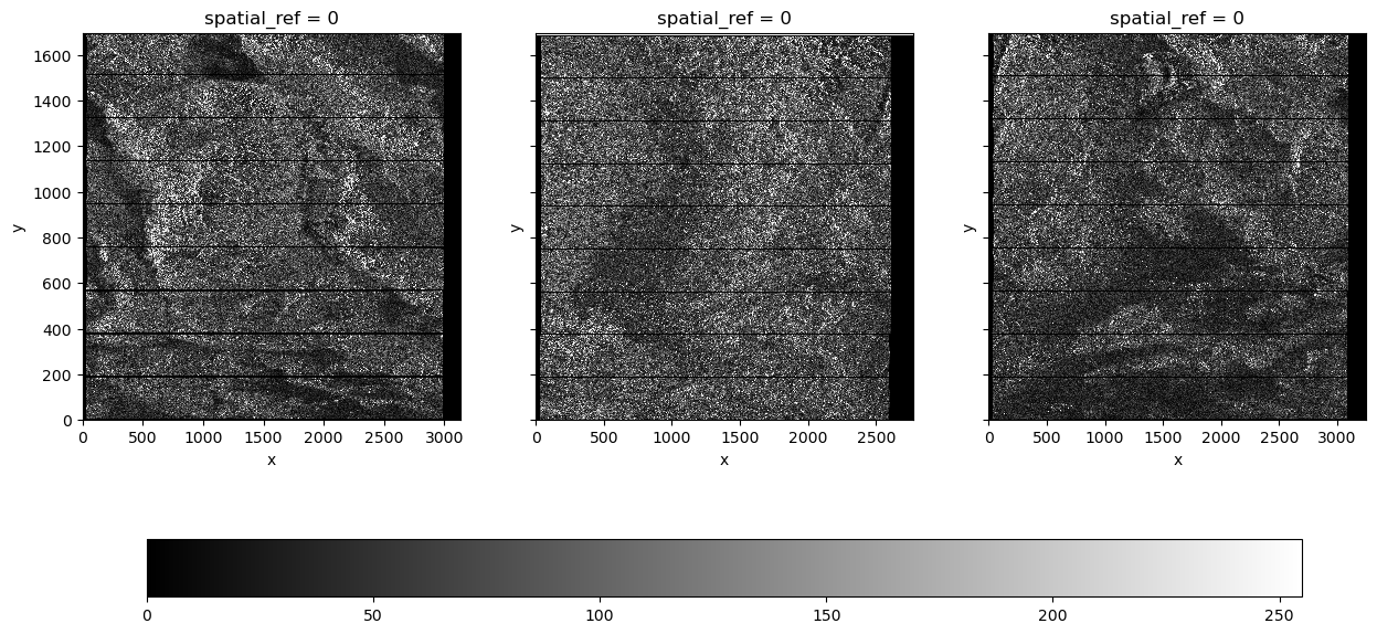
Let’s plot all three sub-swaths to view the full scene acquired by the satellite. The acquisition times for each swath on July 10th, 2019 are the following:

• IW1 at 01:50:01 - 01:50:26

• IW2 at 01:49:59 - 01:50:24

• IW3 at 01:50:00 - 01:50:25

fig, ax = plt.subplots(1, 3, figsize=(15, 7), sharey=True)

datasets = [iw1_ds, iw2_ds, iw3_ds]
val_range = dict(vmin=0, vmax=255, cmap="gray")

for i, ds in enumerate(datasets):
    im = ds.intensity.plot(ax=ax[i], add_colorbar=False, **val_range)
    ax[i].tick_params(axis="both", which="major")

cbar = fig.colorbar(im, ax=ax, orientation="horizontal", shrink=0.9, pad=0.2)

plt.show()

We don’t need all three of the subswaths for our notebook, so we will focus on IW2 and display its intensity and phase measurements.

# Compute the intensity and phase from complex data
cmap_hls = sns.hls_palette(as_cmap=True)

fig, axes = plt.subplots(1, 2, figsize=(15, 6))

ds.intensity.plot(ax=axes[0], cmap="gray", robust=True)
axes[0].set_title("Intensity Measurement of IW2")

ds.phase.plot(ax=axes[1], cmap=cmap_hls)
axes[1].set_title("Phase Measurement of IW2")

plt.tight_layout()

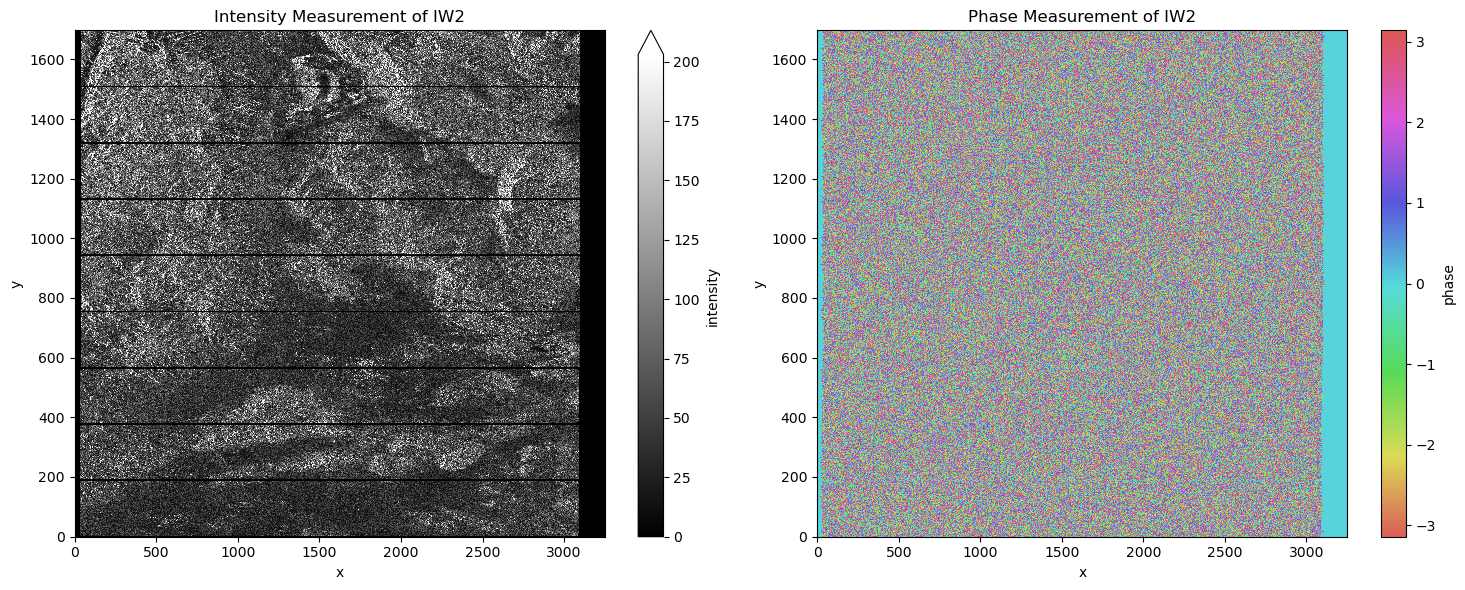
Intensity is represented in an 8-bit format (ranging from 0 to 255), while phase measurements range from \(- \pi\) to \(\pi\) . At first glance, phase does not correspond to easily observable physical properties of the ground. However, the phase becomes incredibly valuable when, for example, it is used comparatively between two successive phase measurements (two Sentinel-1 images acquired at different times over the same area). Here are the processing steps needed to retrieve a difference between the phases of two radar acquisitions:

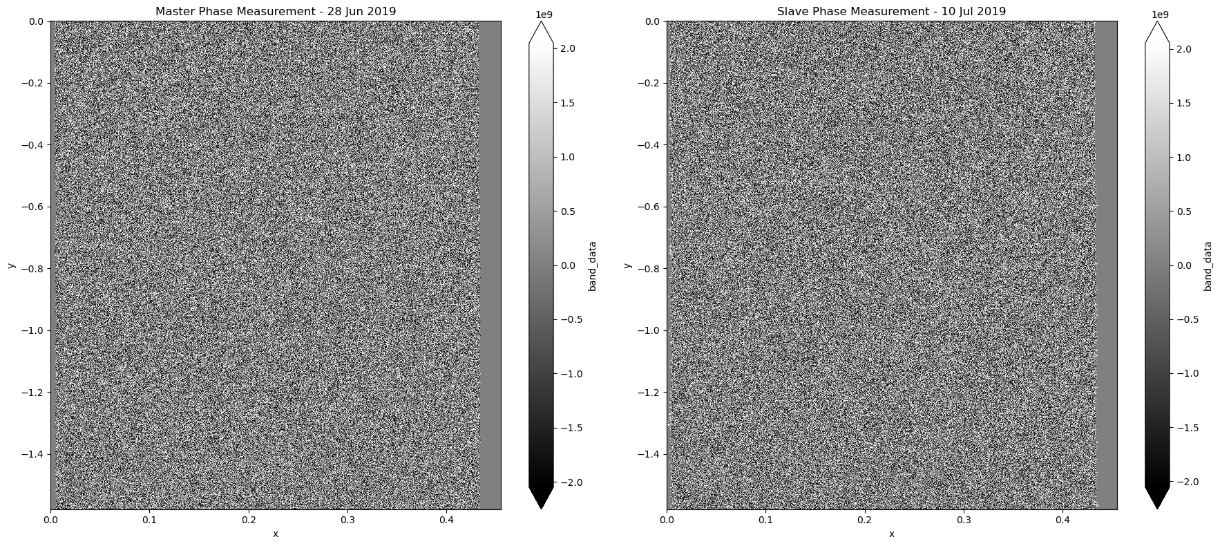
Coregistering

Before creating an interferogram, measurements from two different dates need to be coregistered. This means that each pixel from the two acquisitions must be precisely aligned so that they are representing the same ground object. Accurate and successful co-registration of the two (or more) images is vital for interferometry processing. We call the “master” image the reference image (typically the earliest acquisition in time) to which we coregister the “slave” image (typically acquired later in time).

coregistered_ds = cat.coreg.read()

fig, axes = plt.subplots(1, 2, figsize=(18, 8))
coregistered_ds.band_data.sel(band=1).plot(ax=axes[0], cmap="gray", robust=True)
axes[0].set_title("Master Phase Measurement - 28 Jun 2019")

coregistered_ds.band_data.sel(band=2).plot(ax=axes[1], cmap="gray", robust=True)
axes[1].set_title("Slave Phase Measurement - 10 Jul 2019")

plt.tight_layout()

Interferogram Formation and Coherence Estimation

The interferogram formation process combines the amplitudes of both images and calculates the difference between their respective phases at each SAR image pixel (cross-multiplication of the master image with the complex conjugate of the slave image).

After building up the interferogram, we have to take into account the presence of other contributing terms that could hinder our goal of measuring the surface deformation due to the earthquake. For example, we need to subtract from the interferogram the flat-earth phase contribution, which is a signal contribution due to the curvature of the Earth’s surface. This is here done automatically through the SNAP software operators.

In general, the accuracy of interferometric measurements are influenced by many contributors that could result in a loss of coherence. But what is coherence? It is a measure of phase correlation between the master and slave image. Interferometric coherence (γ) can be expressed as:

\[γ = γ_{proc}*γ_{geom}*γ_{vol}*γ_{SNR}*γ_{temp}\]

where \(γ_{proc}\) refers to inaccuracies in the processing (e.g., coregistration errors), \(γ_{geom}\) refers to the baseline decorrelation (different position of satellites during the two acquisitions), \(γ_{vol}\) refers to volume decorrelation (vegetation related), \(γ_{SNR}\) refers to the radar instrument thermal noise and \(γ_{temp}\) refers to the decorrelation caused by change of position of the objects in the scene during the time interval of the images acquisitions (e.g., plant growth, wind-induced movements or ground deformation due to earthquakes, landslides).

Therefore, we can conclude that interferometric accuracy is sensitive to many processes, hence isolating the ground deformation signal involves several operations. On the other hand, interferometric coherence sensitivity could be exploited to track and map phenomena that cause its degradation (e.g., vegetation features, and water content).

interferogram_ds = cat.inter.read()

cmap_hls_hex = sns.color_palette("hls", n_colors=256).as_hex()

interferogram_ds = interferogram_ds.where(interferogram_ds != 0)
igf_da = interferogram_ds.sel(band=1).band_data
coh_da = interferogram_ds.sel(band=2).band_data

# Invert y axis
igf_da["y"] = igf_da.y[::-1]
coh_da["y"] = coh_da.y[::-1]

igf_plot = igf_da.hvplot.image(
    x="x",
    y="y",
    cmap=cmap_hls_hex,
    width=600,
    height=600,
    dynamic=False,
)

coh_plot = coh_da.hvplot.image(
    x="x",
    y="y",
    cmap="viridis",
    width=600,
    height=600,
    dynamic=False,
).opts(clim=(0, 1))

(igf_plot + coh_plot).opts(shared_axes=True)