Reverend Bayes updates our Belief in Flood Detection

How an 275 year old idea helps map the extent of floods

Image from wikipedia

Note

This notebook contains interactive elements. The full interactive elements can only be viewed on Binder by clicking on the Binder badge or 🚀 button.

Overview

This notebook explains how microwave (\(\sigma^0\)) backscattering can be used to map the extent of a flood. We replicate in this exercise the work of [1] on the TU Wien Bayesian-based flood mapping algorithm.

Prerequisites

Concepts	Importance	Notes
Intro to xarray	Necessary
Intro to Harmonic parameters	Necessary
Documentation hvPlot	Helpful	Interactive plotting
Documentation odc-stac	Helpful	Data access

Time to learn: 10 min

Imports

import datetime

import holoviews as hv
import hvplot.pandas
import hvplot.xarray
import numpy as np
import pandas as pd
import panel as pn
import pystac_client
import rioxarray  # noqa: F401
import xarray as xr
from bokeh.models import FixedTicker
from odc import stac as odc_stac
from scipy.stats import norm

pn.extension()
hv.extension("bokeh")

Greece Flooding 2018

In this exercise we will replicate the case study of the above mentioned paper, the February 2018 flooding of the Greek region of Thessaly.

time_range = "2018-02-28T04:00:00Z/2018-02-28T05:00:00Z"
minlon, maxlon = 21.93, 22.23
minlat, maxlat = 39.47, 39.64
bounding_box = [minlon, minlat, maxlon, maxlat]

From Backscattering to Flood Mapping

In the following lines we create a map with microwave backscattering values.

# | label: fig-area
# | fig-cap: Area targeted for $\sigma^0$ backscattering is the Greek region of Thessaly, which experienced a major flood in February of 2018.
mrs_view = flood_dc.sig0.hvplot.image(
    x="x", y="y", cmap="viridis", geo=True, tiles=True
).opts(frame_height=400)
mrs_view

Microwave Backscattering over Land and Water

Reverend Bayes was concerned with two events, one (the hypothesis) occurring before the other (the evidence). If we know its cause, it is easy to logically deduce the probability of an effect. However, in this case we want to deduce the probability of a cause from an observed effect, also known as “reversed probability”. In the case of flood mapping, we have \(\sigma^0\) backscatter observations over land (the effect) and we want to deduce the probability of flooding (\(F\)) and non-flooding (\(NF\)).

In other words, we want to know the probability of flooding \(P(F)\) given a pixel’s \(\sigma^0\):

\[P(F|\sigma^0)\]

and the probability of a pixel being not flooded \(P(NF)\) given a certain \(\sigma^0\):

\[P(NF|\sigma^0).\]

Bayes showed that these can be deduced from the observation that forward and reversed probability are equal, so that:

\[P(F|\sigma^0)P(\sigma^0) = P(\sigma^0|F)P(F)\]

and

\[P(NF|\sigma^0)P(\sigma^0) = P(\sigma^0|NF)P(NF).\]

The forward probability of \(\sigma^0\) given the occurrence of flooding (\(P(\sigma^0|F)\)) and \(\sigma^0\) given no flooding (\(P(\sigma^0|NF)\)) can be extracted from past information on backscattering over land and water surfaces. As seen in the sketch below , the characteristics of backscattering over land and water differ considerably.

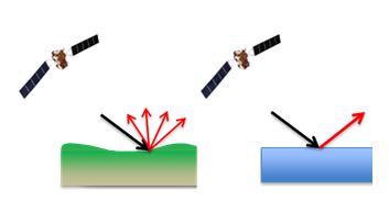Schematic backscattering over land and water. Image from Geological Survey Ireland {#fig-sat}

Likelihoods

The so-called likelihoods of \(P(\sigma^0|F)\) and \(P(\sigma^0|NF)\) can thus be calculated from past backscattering information. In the following code chunk we define the functions calc_water_likelihood and calc_land_likelihood to calculate the water and land likelihood’s of a pixel, based on the Xarray datasets for the PLIA and HPAR, respectively.

def calc_water_likelihood(sigma, x=None, y=None):
    """
    Calculate water likelihoods.

    Parameters
    ----------
    sigma: float|array
        Sigma naught value(s)
    x: float|array
        Longitude
    y: float|array
        Latitude

    Returns
    -------
    numpy array
    """
    point = flood_dc.sel(x=x, y=y, method="nearest")
    wbsc_mean = point.MPLIA * -0.394181 + -4.142015
    wbsc_std = 2.754041
    return norm.pdf(sigma, wbsc_mean.to_numpy(), wbsc_std)


def expected_land_backscatter(data, dtime_str):
    w = np.pi * 2 / 365
    dt = datetime.datetime.strptime(dtime_str, "%Y-%m-%d")
    t = dt.timetuple().tm_yday
    wt = w * t

    M0 = data.M0
    S1 = data.S1
    S2 = data.S2
    S3 = data.S3
    C1 = data.C1
    C2 = data.C2
    C3 = data.C3
    hm_c1 = (M0 + S1 * np.sin(wt)) + (C1 * np.cos(wt))
    hm_c2 = (hm_c1 + S2 * np.sin(2 * wt)) + C2 * np.cos(2 * wt)
    hm_c3 = (hm_c2 + S3 * np.sin(3 * wt)) + C3 * np.cos(3 * wt)
    return hm_c3


def calc_land_likelihood(sigma, x=None, y=None):
    """
    Calculate land likelihoods.

    Parameters
    ----------
    sigma: float|array
        Sigma naught value(s)
    x: float|array
        Longitude
    y: float|array
        Latitude

    Returns
    -------
    numpy array
    """
    point = flood_dc.sel(x=x, y=y, method="nearest")
    lbsc_mean = expected_land_backscatter(point, "2018-02-01")
    lbsc_std = point.STD
    return norm.pdf(sigma, lbsc_mean.to_numpy(), lbsc_std.to_numpy())

Without going into the details of how these likelihoods are calculated, you can hover over a pixel of the map to plot the likelihoods of \(\sigma^0\) being governed by land or water. For reference we model the water and land likelihoods (model_likelihoods) over a range of \(\sigma^0\) values.

# | label: fig-lik
# | fig-cap: Likelihoods for $\sigma^0$ being associated with land or water for 1 pixel in the Greek area of Thessaly. Likelihoods are calculated over a range of $\sigma^0$. The pixel's observed $\sigma^0$ is given with a vertical line. Hover on the map to re-calculate and update this figure for another pixel in the study area.


def model_likelihoods(sigma=(-30, 0), x=None, y=None):
    """
    Model likelihoods over a range of sigma naught.

    Parameters
    ----------
    sigma: tuple
        Minimum and maximum for range of sigma naught values
    x: float|array
        Longitude
    y: float|array
        Latitude

    Returns
    -------
    Pandas Datafrane
    """
    sigma = np.arange(sigma[0], sigma[1], 0.1)
    land_likelihood = calc_land_likelihood(sigma=sigma, x=x, y=y)
    water_likelihood = calc_water_likelihood(sigma=sigma, x=x, y=y)
    point = flood_dc.sel(x=x, y=y, method="nearest")
    return pd.DataFrame(
        {
            "sigma": sigma,
            "water_likelihood": water_likelihood,
            "land_likelihood": land_likelihood,
            "observed": np.repeat(point.sig0.values, len(land_likelihood)),
        }
    )


pointer = hv.streams.PointerXY(source=mrs_view.get(1), x=22.1, y=39.5)

likelihood_pdi = hvplot.bind(
    model_likelihoods, x=pointer.param.x, y=pointer.param.y
).interactive()

view_likelihoods = (
    likelihood_pdi.hvplot("sigma", "water_likelihood", ylabel="likelihoods").dmap()
    * likelihood_pdi.hvplot("sigma", "land_likelihood").dmap()
    * likelihood_pdi.hvplot("observed", "land_likelihood").dmap()
).opts(frame_height=200, frame_width=300)

view_likelihoods + mrs_view.get(1)

Posteriors

Having calculated the likelihoods, we can now move on to calculate the probability of (non-)flooding given a pixel’s \(\sigma^0\). These so-called posteriors need one more piece of information, as can be seen in the equation above. We need the probability that a pixel is flooded \(P(F)\) or not flooded \(P(NF)\). Of course, these are the figures we’ve been trying to find this whole time. We don’t actually have them yet, so what can we do? In Bayesian statistics, we can just start with our best guess. These guesses are called our “priors”, because they are the beliefs we hold prior to looking at the data. This subjective prior belief is the foundation Bayesian statistics, and we use the likelihoods we just calculated to update our belief in this particular hypothesis. This updated belief is called the “posterior”.

Let’s say that our best estimate for the chance of flooding versus non-flooding of a pixel is 50-50: a coin flip. We now can also calculate the probability of backscattering \(P(\sigma^0)\), as the weighted average of the water and land likelihoods, ensuring that our posteriors range between 0 to 1.

The following code block shows how we calculate the priors.

def calc_posteriors(sigma, x=None, y=None):
    """
    Calculate posterior probability.

    Parameters
    ----------
    sigma: float|array
        Sigma naught value(s)
    x: float|array
        Longitude
    y: float|array
        Latitude

    Returns
    -------
    Tuple of two Numpy arrays
    """
    land_likelihood = calc_land_likelihood(sigma=sigma, x=x, y=y)
    water_likelihood = calc_water_likelihood(sigma=sigma, x=x, y=y)
    evidence = (water_likelihood * 0.5) + (land_likelihood * 0.5)
    water_posterior = (water_likelihood * 0.5) / evidence
    land_posterior = (land_likelihood * 0.5) / evidence
    return water_posterior, land_posterior

We can plot the posterior probabilities of flooding and non-flooding again and compare these to pixel’s measured \(\sigma^0\). For reference we model the flood and non-flood posteriors (model_posteriors) over a range of \(\sigma^0\) values. Hover on a pixel to calculate the posterior probability.

# | label: fig-post
# | fig-cap: Posterior probabilities for $\sigma^0$ of 1 pixel being associated with land for water in the Greek area of Thessaly. Hover on the map to re-calculate and update this figure for another pixel in the study area.


def model_posteriors(sigma=(-30, 0), x=None, y=None):
    """
    Model posterior probabilities over a range of sigma naught.

    Parameters
    ----------
    sigma: tuple
        Minimum and maximum for range of sigma naught values
    x: float|array
        Longitude
    y: float|array
        Latitude

    Returns
    -------
    Pandas Datafrane
    """
    bays_pd = model_likelihoods(sigma=sigma, x=x, y=y)
    sigma = np.arange(sigma[0], sigma[1], 0.1)
    bays_pd["f_post_prob"], bays_pd["nf_post_prob"] = calc_posteriors(
        sigma=sigma, x=x, y=y
    )
    return bays_pd


posterior_pdi = hvplot.bind(
    model_posteriors, x=pointer.param.x, y=pointer.param.y
).interactive()

view_posteriors = (
    posterior_pdi.hvplot("sigma", "f_post_prob", ylabel="posteriors").dmap()
    * posterior_pdi.hvplot("sigma", "nf_post_prob").dmap()
    * posterior_pdi.hvplot("observed", "nf_post_prob").dmap()
).opts(frame_height=200, frame_width=300)

(view_likelihoods + view_posteriors).cols(1) + mrs_view.get(1)

Flood Classification

We are now ready to combine all this information and classify the pixels according to the probability of flooding given the backscatter value of each pixel. Here we just look whether the probability of flooding is higher than non-flooding:

def bayesian_flood_decision(sigma, x=None, y=None):
    """
    Bayesian decision.

    Parameters
    ----------
    sigma: float|array
        Sigma naught value(s)
    x: float|array
        Longitude
    y: float|array
        Latitude

    Returns
    -------
    Xarray DataArray
    """
    f_post_prob, nf_post_prob = calc_posteriors(sigma=sigma, x=x, y=y)
    return xr.where(
        np.isnan(f_post_prob) | np.isnan(nf_post_prob),
        np.nan,
        np.greater(f_post_prob, nf_post_prob),
    )

Hover on a point in the below map to see the likelihoods and posterior distributions (in the left-hand subplots).

# | label: fig-clas
# | fig-cap: Flood extent of the Greek region of Thessaly based on Bayesian probabilities are shown on the map superimposed on an open street map. Hover over a pixel to generate the point's water and land likelihoods as well as the posterior probabilities.


flood_dc["decision"] = (
    ("y", "x"),
    bayesian_flood_decision(flood_dc.sig0, flood_dc.x, flood_dc.y),
)

colorbar_opts = {
    "major_label_overrides": {
        0: "non-flood",
        1: "flood",
    },
    "ticker": FixedTicker(ticks=[0, 1]),
}
flood_view = flood_dc.decision.hvplot.image(
    x="x", y="y", rasterize=True, geo=True, cmap=["rgba(0, 0, 1, 0.1)", "darkred"]
).opts(frame_height=400, colorbar_opts={**colorbar_opts})
mrs_view.get(0) * flood_view

Reverend Bayes updates our Belief in Flood Detection

Overview

Prerequisites

Imports

Greece Flooding 2018

EODC STAC Catalog

Sigma naught

Harmonic Parameters

Projected Local Incidence Angles