Goal
The cookbook guides users in identifying and tracking meteorological features across space and time using three methods: Matplotlib, SciPy, and Scikit.
Figure 1:Scikit tracked SLP features over 12 hours
Object Identification and Tracking Method
This approach is appropriate for our case because the target features are spatially coherent threshold-defined regions, rather than textures, edges, or learned image classes. We are not trying to classify scenes using a trained model. Instead, we identify closed or contiguous regions that satisfy a physically motivated criterion and then follow those regions over time.
This makes connected-component labeling simpler, more transparent, and easier to defend than more complex image-processing or machine-learning methods.
The tracking step links labeled objects between consecutive time steps. For each object at time (t), its spatial mask is compared with objects at time (t+1). If two objects overlap sufficiently, they are assigned to the same track. If no sufficient overlap is found, a new track is started.
What Features Can You Track?
- Extratropical cyclones
- Large-scale low-pressure systems that impact Earth’s midlatitudes typically associated with meridional temperature advection, heavy precipitation, and strong wind.
- Tropical cyclones
- Intense low-pressure systems impacting the tropical regions, associated with very heavy rain and intense, damaging winds.
- Mesoscale convective systems (MCS)
- A continuous complexes of thunderstorms that occur in atmospheric environments with convective instability and vertical wind shear.
- Clouds
- (work in progress)
What is the main difference between Matplotlib, SciPy, and Scikit for tracking these features?
Matplotlib
The contour algorithm in Matplotlib Hunter, 2007 is boundary-based. It runs a marching-squares pass over the field: for each 2×2 block of grid points, it checks which corners are below 1005 hPa, then draws the iso-line where the field crosses that value, placing each vertex by linear interpolation along the cell edges. So the output is a set of polygon paths connecting grid points, with sub-grid precision, vector geometry, and the feature defined by its outline.
You get the boundary for free, but no labeled interior points: area, centroid, and overlap all have to come from polygon operations (shoelace, point-in-polygon, or Shapely).
At a diagonal saddle like the one above, marching squares is genuinely ambiguous and resolves it with a tie-break rule, so the contour can pinch into one loop or two, depending on the values and the chosen disambiguation.
SciPy
SciPy Virtanen et al., 2020 is an open-source Python Library that builds upon Numpy to preform technical, scientific, and mathmatical computuations. We will be utilizing Scipy.ndimage in our cookbook.
Scipy.ndimage provides general image processing and analysis functions for working with n-dimensional numpy arrays.
It is often used in image filtering to apply standard kernels for smoothing or edge detection.
The labeling step identifies groups of neighboring non-background grid cells as individual objects. As part of the labeling step, one must create a structure that serves as the criterion for how many grid cells must border one another to be considered an object.
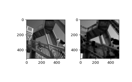
Figure 2:SciPy Minimum Filter Examples
Scikit
Scikit or Scikit-learn Pedregosa et al., 2011 is an open-source machine learning library for Python. It builds upon Numpy, SciPy, and Matplotlib. It provides a clean interface for newer users.
Skimage.measure
Label - two pixels can be connected if they have the same value and are neighbors. The value is based on the maximum number of orthogonal hops (steps) required to reach them. In our case, we use 2-connectivity, meaning there can be up to 2 hops before a node is considered a neighbor.
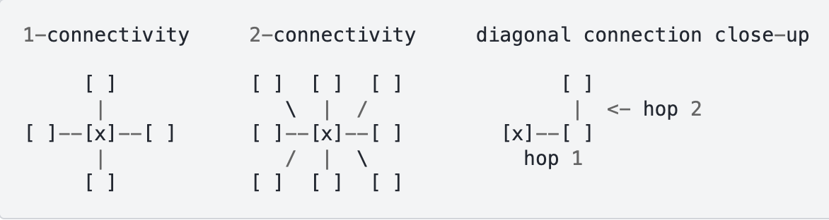
Figure 3:Scikit Label Feature Example
How to Access ERA5 Data
For our purposes, we will look at the ERA5 datasets provided by Copernicus. This data provides an accurate and seamless record of Earth’s atmosphere, utilizing computer models and global observations.
The easiest way to download their data is to navigate to Climate Data Store and filter to the type of data you want to work with. For this notebook, the dataset is already provided.
In our appendix we also show how you can stream the same ERA5 data directly from the cloud.
Resources
Common Abbreviations Used
- ERA5
- European Centre for Medium-Range Weather Forecasts (ECMWF) Reanalysis fifth generation
- QPF
- Quantitative Precipitation Forecast.
- SLP
- Sea Level Pressure
- ETC
- Extratropical Cyclone
- MCS
- Mesoscale Convective Systems
- Hunter, J. D. (2007). Matplotlib: A 2D Graphics Environment. Computing in Science & Engineering, 9(3), 90–95. 10.1109/MCSE.2007.55
- Virtanen, P., Gommers, R., Oliphant, T. E., Haberland, M., Reddy, T., Cournapeau, D., Burovski, E., Peterson, P., Weckesser, W., Bright, J., van der Walt, S. J., Brett, M., Wilson, J., Millman, K. J., Mayorov, N., Nelson, A. R. J., Jones, E., Kern, R., Larson, E., … Vázquez-Baeza, Y. (2020). SciPy 1.0: fundamental algorithms for scientific computing in Python. Nature Methods, 17(3), 261–272. 10.1038/s41592-019-0686-2
- Pedregosa, F., Varoquaux, G., Gramfort, A., Michel, V., Thirion, B., Grisel, O., Blondel, M., Prettenhofer, P., Weiss, R., Dubourg, V., Vanderplas, J., Passos, A., Cournapeau, D., Brucher, M., Perrot, M., & Duchesnay, E. (2011). Scikit-learn: Machine Learning in Python. Journal of Machine Learning Research, 12, 2825–2830.